| Issue |
A&A
Volume 617, September 2018
|
|
|---|---|---|
| Article Number | A140 | |
| Number of page(s) | 14 | |
| Section | Cosmology (including clusters of galaxies) | |
| DOI | https://doi.org/10.1051/0004-6361/201732240 | |
| Published online | 02 October 2018 | |
Ambiguities in gravitational lens models: impact on time delays of the source position transformation
Argelander-Institut für Astronomie,
Auf dem Hügel 71,
53121
Bonn, Germany
e-mail: This email address is being protected from spambots. You need JavaScript enabled to view it.
Received:
6
November
2017
Accepted:
11
December
2017
Abstract
The central ambition of the modern time delay cosmography consists in determining the Hubble constant H0 with a competitive precision. However, the tension with H0 obtained from the Planck satellite for a spatially flat ΛCDM cosmology suggests that systematic errors may have been underestimated. The most critical of these errors probably comes from the degeneracy existing between lens models that was first formalized by the well-known mass-sheet transformation (MST). In this paper, we assess to what extent the source position transformation (SPT), a more general invariance transformation which contains the MST as a special case, may affect the time delays predicted by a model. To this aim, we have used pySPT, a new open-source python package fully dedicated to the SPT that we present in a companion paper. For axisymmetric lenses, we find that the time delay ratios between a model and its SPT-modified counterpart simply scale like the corresponding source position ratios, Δtˆ/Δt ≈ βˆ/β, regardless of the mass profile and the isotropic SPT. Similar behavior (almost) holds for nonaxisymmetric lenses in the double image regime and for opposite image pairs in the quadruple image regime. In the latter regime, we also confirm that the time delay ratios are not conserved. In addition to the MST effects, the SPT-modified time delays deviate in general no more than a few percent for particular image pairs, suggesting that its impact on time delay cosmography seems not be as crucial as initially suspected. We also reflected upon the relevance of the SPT validity criterion and present arguments suggesting that it should be reconsidered. Even though a new validity criterion would affect the time delays in a different way, we expect from numerical simulations that our conclusions will remain unchanged.
Key words: cosmological parameters / gravitational lensing: strong
© ESO 2018
1 Introduction
The use of the gravitational lensing phenomenon as a cosmological tool offers an independent way to probe the nature of the universe (for the early work, see Blandford & Narayan 1992). To date, numerous weak and strong lensing observations have been employed to infer the fundamental cosmological parameters with an increasingly competitive precision. In the strong lensing regime, Refsdal (1964) established that multiple-image systems can theoretically be used to infer the Hubble parameter H0. The method relies upon the idea that the propagation time of light rays emitted from a background source (typically an active galactic nucleus, AGN) towards the observer differs from one lensed image to another. The corresponding difference in arrival times, known as the time delay, is inversely proportional to H0. This idea lays the basis of the modern time delay cosmography, which has been extensively addressed in literature; see, for example, the recent review Treu & Marshall (2016) and references therein.
For sake of clarity, we recall few key results of the well-known theory of time delays. Relative to an unperturbed ray emitted by a source located at β, the extra light travel time T(θ) at an image position θ is formally defined by
![Mathematical equation: \begin{equation*} T(\boldsymbol{\theta}) = \frac{D_{\mathrm{\Delta} t}}{c} \left\{\frac{1}{2} \left[\boldsymbol{\theta} - \boldsymbol{\beta}(\boldsymbol{\theta})\right]^2 - \psi(\boldsymbol{\theta}) \right\} \eqqcolon \frac{D_{\mathrm{\Delta} t}}{c}\ \tau(\boldsymbol{\theta}) ,\end{equation*}](/articles/aa/full_html/2018/09/aa32240-17/aa32240-17-eq2.png) (1)
(1)
where ψ(θ) is the deflection potential produced by a dimensionless surface mass density κ(θ) = ∇2ψ(θ)∕2, τ(θ) is known as the Fermat potential, and DΔt is referred to as the time delay distance
 (2)
(2)
where zd is the redshift of the deflector and D is the angular diameter distances between the observer and deflector (d), observer and source (s), and deflector and source (ds). In Eq. (1), the first term in brackets describes the geometrical deviation of the light ray due to the lens, whereas the second describes the time delay that a ray experiences as it crosses the deflection potential. The relative time delay Δ tij between a pair of lensed images θi and θj is obtained by differencing the corresponding extra light travel time:
![Mathematical equation: \begin{equation*} \mathrm{\Delta} t_{ij} = T(\boldsymbol{\theta}_i) - T(\boldsymbol{\theta}_j) = \frac{D_{\mathrm{\Delta} t}}{c} \left[\tau(\boldsymbol{\theta}_i) - \tau(\boldsymbol{\theta}_j)\right] \eqqcolon \frac{D_{\mathrm{\Delta} t}}{c} \mathrm{\Delta} \tau_{ij}.\end{equation*}](/articles/aa/full_html/2018/09/aa32240-17/aa32240-17-eq4.png) (3)
(3)
From Eq. (3), H0 inference can be conceptually performed by constraining the time delay distance DΔt, provided that both accurate time delay measurements and a mass model which predicts Δ τij can be obtained. At present, a few percent precision time delays have been measured for several multiple-image systems based on different light curve analysis methods (see e.g., Vuissoz et al. 2008; Paraficz & Hjorth 2010; Courbin et al. 2011; Fohlmeister et al. 2013; Eulaers et al. 2013; Tewes et al. 2013; Rathna Kumar et al. 2013; Bonvin et al. 2017; Akhunov et al. 2017). In the foreseeable future, we can expect thousands of lensed quasars to be discovered by the next generation of instruments (Jean et al. 2001; Coe & Moustakas 2009; Oguri & Marshall 2010; Finet et al. 2012, 2015; Liao et al. 2015; Finet & Surdej 2016). Among them, numerous suitable candidates for robust time delay measurements should lead the time delay cosmography to the next level. However, constraining the lens mass distribution turns out to be as decisive as measuring time delays with high precision. Given a measured time delay between two lensed images, more concentrated mass distributions lead to shorter time delay distance estimations, hence to larger values of H0 (Kochanek 2002). The Fermat potential difference Δτij is primarily sensitive to the strong lensing effects produced by the main lens. However, a realistic time delay cosmography should also consider the lensing effects of any external mass structures located in the vicinity of the main lens, as well as along the line of sight (LOS; e.g., Seljak 1994; Bar-Kana 1996). If the LOS mass effects are sufficiently small, they can be approximated by an external shear and an external convergence, usually denoted as κext, which need to be characterized1 (see e.g., Keeton 2003; Fassnacht et al. 2006; Suyu et al. 2010, 2013; Wong et al. 2011, 2017). Otherwise, these external mass structures need to be explicitly included in the mass model, for instance by considering the full multi-plane lensing formalism (Schneider 2014b; McCully et al. 2014, 2016).
As firstshown in Falco et al. (1985), the dimensionless surface mass density κ(θ) and the class of mass models κλ(θ) defined as
 (4)
(4)
along with the corresponding unobservable source rescaling β → λ β, lead to identical lensing observables, except for the time delays between pairs of lensed images which are transformed such that Δ t → λ Δt. If not broken, this degeneracy, referred to as the mass-sheet transformation (MST), may significantly affect cosmographic inferences, including H0 (see e.g., Gorenstein et al. 1988; Saha 2000; Wucknitz 2002; Koopmans et al. 2003; Liesenborgs & De Rijcke 2012; Schneider & Sluse 2013; Schneider 2014a,b; Xu et al. 2016). It is worth mentioning that the external convergence κext is based on physical effects whereas the MST (Eq. (4)) stems from a pure mathematical degeneracy (Schneider & Sluse 2013; hereafter SS13). Different solutions have been proposed to reduce the degeneracy induced by the MST in time delay cosmography (see e.g., Birrer et al. 2016; Treu & Marshall 2016, and references therein). A commonly used method consists in assuming a specific lens model, typically a power-law, and independently estimating the lens mass with the measurement of its velocity dispersion. However, SS13 have shown experimentally that two different classes of galaxy models with compatible velocity dispersions were able to reproduce equally well a set of image positions, but predicted significantly different time delays. Furthermore, because the time delay ratios were not constant, they suggested that the transformation between these two models was not exactly an MST but a more general one. This has naturally raised some concerns about the reliability of the H0 determination from time delay cosmography.
Schneider & Sluse (2014; hereafter SS14) laid the theoretical basis for an approximate invariance transformation, the so-called source-position transformation (SPT), of which the MST is a special case. Unruh et al. (2017; hereafter USS17) explored further its properties, such as defining a criterion to determine whether an SPT is valid or not and exploring the density profile of SPT-modified mass distributions. They also pointed out that the degeneracy found experimentally in SS13 between the two models mimics an SPT, which thereby confirmed that it occurs in real lens modeling. To date, it is not clear whether the conclusions drawn in SS13 and SS14 about time delays and H0 could be generalized to other mass distributions modified under exact SPTs or only reflect the behavior of a very special case. In this paper, we address this question by studying how time delays are sensitive to the effects of the SPT.
This paper is organized as follows. For readers who are not familiar with the SPT, we outline its basic principles in Sect. 2. In particular, we recall the importance of identifying a validity criterion. Owing to the valuable insight it offers for more general cases, we consider the SPT-modified time delays for axisymmetric lenses in Sect. 3. For nonaxisymmetric lenses, we discuss in Sect. 4 the relevance of the validity criterion defined in USS17 and analyze the SPT-modified time delays in detail. We summarize our findings and conclude in Sect. 5.
2 The principle of the source position transformation
This section focuses on the principle of the SPT and the most recent theoretical results. For a detailed discussion, the reader is referred to SS14 and USS17. All the analytical results presented in this paper have been implemented into a user friendly python package called pySPT. All the numerical results and figures have also been obtained from pySPT without using any extra software. For an overall description of the package, we refer the reader to the companion paper Wertz & Orthen (2018).
The basic idea underlying the SPT can be simply summarized as follows. A given general mass distribution κ(θ) defines a deflection law α(θ) which describes how the light paths are affected in the vicinity of the deflector. The n lensed image angular positions θi of a point-like source at unobservable position β are those which satisfy the lens equation β = θi −α(θi). Then, from astrometric observations, we can infer the constraints
 (5)
(5)
for all 1 ≤ i < j ≤ n, leading to the mapping θi(θ1) defined by the relative image positions of the same source. The SPT addresses the following question: can we define an alternative deflection law, denoted as  , which preserves the mapping θi(θ1) for a uniquesource? If such a deflection law exists, it will necessarily be associated with the alternative source position
  , defining a new lens mapping, in such a way that
 (6)
(6)
An SPT consists in a global transformation of the source plane formally defined by a mapping  which gives rise to the transformed deflection law:
 (7)
(7)
where in the first step we used Eq. (6) and in the last step we inserted the original lens equation. The mapping  is chosen so that it satisfies
  for all β in the region of interest, hence
  is one-to-one. This property of the source mapping guarantees the pairing of images to be conserved. With
  defined thisway, Eq. (6) guarantees that all images of a given source β under the original deflection law α(θ) are also images of the source
  under the modified deflection law
  . Therefore, the mapping θi(θ1) is preserved for all source positions.
From the Jacobi matrix  of the modified lens mapping
  , SS14 have shown that both the magnification ratios of image pairs and their relative shapes remain unchanged under an SPT. In general, the Jacobi matrix
  is not symmetric, which indicates that the modified deflection law
  is not a curl-free field:
 (8)
(8)
where the subscript indices refer to the matrix entries. Therefore,  cannot be in general expressed as the gradient of a deflection potential
  and does not correspond to the deflection produced by a gravitational lens. Thus, there exists no physical mass distribution
  leading to the modified deflection law
  . The only cases for which
  is globally symmetric occur either when the SPT simply reduces to an MST
  , or when axisymmetric lenses are transformed under SPTs corresponding to a general radial stretching of the form
![Mathematical equation: \begin{equation*} \hat{\boldsymbol{\beta}}(\boldsymbol{\beta}) = \left[1 + f(|\boldsymbol{\beta}|) \right] \boldsymbol{\beta},\end{equation*}](/articles/aa/full_html/2018/09/aa32240-17/aa32240-17-eq29.png) (9)
(9)
where f is called the deformation function. For such cases, we can always define  so that
  . However, even in this case there is still no guarantee that
  corresponds to a physical mass distribution. Depending on the SPT, the modified mass profile may become nonmonotic or even non-positive definite in particular regions of the lens plane.
Provided the curl component of  is sufficiently small, it was shown in USS17 that one can define a curl-free deflection law
  which is very similar to
  in the sense that their difference is smaller than the astrometric accuracy εacc of current observations:
 (10)
(10)
in a finite region  where multiple images occur. Therefore,
  can be derived as the gradient of a deflection potential
  , which is caused by a mass distribution
  corresponding to a gravitational lens. The central question of the validity of an SPT was addressed in USS17. Whereas
  yields exactly the same lensed image positions as the original lens,
  does not. Because of observational uncertainties and additional physical reasons such as substructures in the mass distribution, we cannot reproduce observed positions to better than a few milliarcseconds (mas) with a smooth mass model (for a detailed discussion, see SS14). A given SPT
  should be flagged as being valid as long as a corresponding curl-free
  leads to lensed image shifts smaller than a few mas. In this sense, the SPT is only an approximate invariance transformation. The condition (10) was chosen in USS17 as the criterion to assess whether an SPT is valid or not. The relevance of this choice is reconsidered in detail in Sect. 4.1.
Because it will be of practical interest for deriving SPT-modified time delays in the nonaxisymmetric case (see Sect. 4), we recall here the explicit expressions for  and
and  . These can essentially be obtained by formulating the “action”
 (11)
(11)
for which finding a minimum leads to the Neumann problem:
 (12)
(12)
where  represents the boundary curve of
  and n the outward directed normal vector. From Eq. (11), we see that the condition (10) plays a central role in defining a curl-free counterpart
  of the SPT-modified deflection law
  . We also note that the first relation in Eq. (12) implies
  for all
  . The Neumann problem can be solved by means of a Green’s function for which an analytical solution is known when
  is a disk of radius R. Thus, the deflection potential
  evaluated at the position ϑ in the lens plane explicitly reads (Unruh et al. 2017; Wertz & Orthen 2018)
 (13)
(13)
where  is the average of
  on
on  , ds the line element of the boundary curve
  ,
,
![Mathematical equation: \begin{equation*} H_1(\boldsymbol{\vartheta};\boldsymbol{\theta}) = \frac{1}{4 \pi} \left[\ln\left(\frac{\left|\boldsymbol{\vartheta}-\boldsymbol{\theta}\right|^2}{R^2}\right) + \ln\left(1 - \frac{2 \boldsymbol{\vartheta} \cdot \boldsymbol{\theta}}{R^2} + \frac{|\boldsymbol{\vartheta}|^2 |\boldsymbol{\theta}|^2}{R^4}\right) - \frac{|\boldsymbol{\theta}|^2}{R^2} \right],\end{equation*}](/articles/aa/full_html/2018/09/aa32240-17/aa32240-17-eq62.png) (14)
(14)
and
![Mathematical equation: \begin{equation*} H_2(\boldsymbol{\vartheta};\boldsymbol{\theta}) = \frac{1}{4 \pi} \left[2 \ln\left(\frac{\left|\boldsymbol{\vartheta}-\boldsymbol{\theta}\right|^2}{R^2}\right) - 1 \right].\end{equation*}](/articles/aa/full_html/2018/09/aa32240-17/aa32240-17-eq63.png) (15)
(15)
The corresponding deflection angle  can be derived by obtaining the gradient of H1 and H2 with respect to ϑ, which reads
 (16)
(16)
Of course,  and
and  depend on the radius R of the circular region
  and must satisfies the two conditions R > |ϑ| and R not too large to ensure the criterion (10) to be satisfied.
To quantitatively study the impact of the SPT on time delays, it will be necessary to explicitly define a mapping  . We will focus most of this work on an isotropic SPT described by the radial stretching of the form (9). In particular, we will consider the special case where the deformation function f(|β|) is the lowest-order expansion of more general functions:
 (17)
(17)
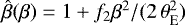
where f0f(0), :=  , and θE is the Einstein angular radius. When f2 = 0, Eq. (17) reduces to f0 and the radial stretching (9) simplifies to a pure MST with λ = 1 + f0. Such as in SS14 and USS17, we only consider SPT parameters which yield to physically meaningful modified mass profiles.
3 Time delays: the axisymmetric case
Owing to its simplicity, the study of how an SPT affects time delays between lensed images produced by an axisymmetric lens provides a valuable insight on the general nonaxisymmetric case. Since α and θ are collinear, the original lens mapping becomes one-dimensional and reads β = θ − α(θ). We set β > 0 and only consider the two outer2 lensed images θA and θB located on opposite sides of the lens center, that is θB < 0 < |θB| < θA. From Eq. (1), we readily deduce the one-dimensional form of the original time delay Δ tAB between the image pair (θA, θB):
![Mathematical equation: \begin{equation*} \mathrm{\Delta} t_{\text{{AB}}} = \frac{D_{\mathrm{\Delta} t}}{c} \Big[\tau(\theta_{\rm{{A}}}) - \tau(\theta_{\rm{{B}}})\Big] \eqqcolon \frac{D_{\mathrm{\Delta} t}}{c} \mathrm{\Delta} \tau_{\text{{AB}}}.\end{equation*}](/articles/aa/full_html/2018/09/aa32240-17/aa32240-17-eq72.png) (18)
(18)
The one-dimensional radial stretching (9) simply reads
![Mathematical equation: \begin{equation*} \hat{\beta}(\beta) = [1 + f(\beta)]\ \beta,\end{equation*}](/articles/aa/full_html/2018/09/aa32240-17/aa32240-17-eq73.png) (19)
(19)
where f(−β) = f(β) to preserve the symmetry. With no loss of generality, 1 + f(β) + β df(β)∕dβ > 0 ensures the SPT to be one-to-one. For the axisymmetric case, the SPT is an exact invariance transformation. Thus, the deflection law  is a curl-free field,
  , and there exists a deflection potential
  such as
 (20)
(20)
where in the second step we used the one-dimensional form of Eq. (7). From Eq. (1), we deduce that the SPT-modified extra light travel time  reads
reads
![Mathematical equation: \begin{equation*} \hat{T}(\theta) = \frac{D_{\mathrm{\Delta} t}}{c} \left[\frac{1}{2} \left(\theta - \hat{\beta}[\beta(\theta)]\right)^2 - \hat{\psi}(\theta) \right] \eqqcolon \frac{D_{\mathrm{\Delta} t}}{c}\ \hat{\tau}(\theta).\end{equation*}](/articles/aa/full_html/2018/09/aa32240-17/aa32240-17-eq79.png) (21)
(21)
From Eqs. (3) and (21), the SPT-modified time delay between image pair (θA, θB) of the same source thus becomes
 (22)
(22)
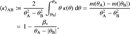
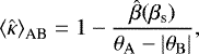
With Eqs. (18) and (22), we show in Sect. 3.1 that the time delay ratios  can be highly simplified, revealing an elegant expression in terms of β and
  , and valid for any axisymmetric lens and deformation function f(β). We also propose an equivalent form of this relation in terms of the original and SPT-modified mean surface mass densities. We illustrate the analytical results with some examples in Sect. 3.2.
3.1 The SPT-modified time delays
After substituting the one-dimensional form of Eqs. (6) and (20) into Eq. (21), the SPT-modified extra light travel time reads 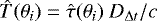 with
with
![Mathematical equation: \begin{equation*} \hat{\tau}(\theta_i) = \frac{1}{2} \Big[\alpha(\theta_i) - f(\beta(\theta_i))\ \beta(\theta_i) \Big]^2 - \psi(\theta_i) + \int_{0}^{\theta_i} f(\beta(\theta))\ \beta(\theta)\ \text{d}\theta,\end{equation*}](/articles/aa/full_html/2018/09/aa32240-17/aa32240-17-eq84.png) (23)
(23)
up to a constant independent of θ, keeping in mind that β(θ) = θ − α(θ). Because of β(θA) = β(θB) =: βs, we have f(β(θA)) = f(β(θB)) = f(βs), and the SPT-modified time delays between the images θA and θB is given by 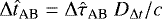 with
with
 (24)
(24)
Due to the lens symmetry, the integral over [θB, |θB|] does not contribute to  . With no loss of generality, we thus integrate from |θB| instead of θB in Eq. (24). To go a step further, the difference ΔτAB between the original Fermat potentials can also be written as

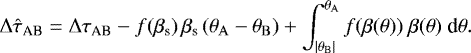
where in the first step we used the original lens equations α(θA) = θA − βs and α(θB) = θB − βs, and in the last step we used dψ(θ)∕dθ = θ − β(θ). Combining Eqs. (24) and (26), we then obtain from Eq. (22) the SPT-modified time delay:
![Mathematical equation: \begin{equation*} \mathrm{\Delta} {\hat{t}}_{\textrm{AB}} = \mathrm{\Delta} {t}_{\textrm{AB}} \left[1 + f(\beta_{\text{s}})\right] + \frac{D_{\mathrm{\Delta} t}}{c}\ {\varepsilon}_{\textrm{AB}},\end{equation*}](/articles/aa/full_html/2018/09/aa32240-17/aa32240-17-eq89.png) (27)
(27)
where we define εAB as
![Mathematical equation: \begin{equation*} {\varepsilon}_{\textrm{AB}} = \int_{|\theta_{\rm{{B}}}|}^{\theta_{\rm{{A}}}} \beta(\theta) \left[f(\beta(\theta)) - f(\beta_{\text{s}})\right]\ \text{d}\theta.\end{equation*}](/articles/aa/full_html/2018/09/aa32240-17/aa32240-17-eq90.png) (28)
(28)
For the special case of a pure MST, the deformation function f is independent of β, namely f(β(θ)) = f(βs) ≡ λ − 1 with  . Therefore, εAB = 0 and we find
 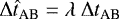 for all axisymmetric lenses, as expected. Considering the radial stretching (19) and a singular isothermal sphere (SIS) lens model, we show explicitly in Appendix A that εAB = 0 also holds for all image pairs (θA, θB), that is for 0 ≤ β < θE. In fact, simple analytical arguments reveal that, in general, εAB remains very small compared to the other terms in Eq. (27) and can be neglected. The demonstration is explained in detail in Appendix B. As a result, the time delay ratios
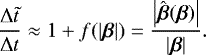
  given in Eq. (27) can be simply approximated by
 (29)
(29)
where we have dropped the subscript AB keeping in mind that the equation holds only for time delay ratios between the same pair of lensed images corresponding to the source  and β. For a given radial stretching, Eq. (29) shows that the ratios between SPT-modified and original time delays scale basically like
  , implying that they depend explicitly on the deformation function f(β), as it is the case for the MST.
As written, Eq. (29) misleadingly suggests that the time delay ratio is insensitive to the original lens profile κ. Consider two original radial mass profiles κ(1) and κ(2), which are not related under an SPT, and consider a source position β. We locate the corresponding pairs of brighter lensed images by  and
and  . For a given deformation function f(β), Eq. (29) says that
 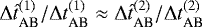 , but the two time delay ratios are evaluated at two different pairs of positions which depend on the lens models, that is
  and
and  . When κ(2) corresponds to a modified version of κ(1) under the SPT
 ![Mathematical equation: $\hat{\beta}(\beta) = [1 + g(\beta)]\ \beta$](/articles/aa/full_html/2018/09/aa32240-17/aa32240-17-eq102.png) (with g(β) satisfying the conditions given after Eq. (19)), we have
(with g(β) satisfying the conditions given after Eq. (19)), we have  and
and  . However, this case can be reduced to an original radial mass profile κ(1) deformed by an SPT that is defined as the composition of two other SPTs such as
 ![Mathematical equation: $\hat{\beta}(\beta) = [1 + h(\beta)]\ \beta$](/articles/aa/full_html/2018/09/aa32240-17/aa32240-17-eq105.png) with h(β) = [1 + f(β)][1 + g(β)] − 1. Thus, this leads to
with h(β) = [1 + f(β)][1 + g(β)] − 1. Thus, this leads to 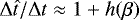 , in agreement with Eq. (29).
The SPT-modified mass profile  of a radial profile κ is also radial (SS14). Therefore, time delays ΔtAB and
  should depend only on the image positions and the corresponding surface mass densities in the annulus defined between the images. In particular for Δ tAB, the major contribution comes from the mean surface mass density
  in the annulus
  (Gorenstein et al. 1988; Kochanek 2002, 2006). We will show next that the time delay ratios (29) can be expressed only in terms of
  and the corresponding SPT-modified
  . First, we can easily show that
 (30)
(30)
where in the last step we used m(θ) = θ α(θ), α(θA) = θA − βs, and α(θB) = θB − βs. Similarly, we can easily deduce that
 (31)
(31)
where we first used  and Eq. (20), then α(θA) = θA − βs and α(θB) = θB − βs. Combining Eqs. (29) and (31), we thus obtain for the time delay ratio in terms of mean surface mass densities:
 (32)
(32)
where we have once again dropped the AB keeping in mind that the mean surface mass densities are evaluated in the annulus defined by the inner and outer radii |θB| and θA, respectively. As expected, Eq. (32) shows that the ratio between SPT-modified and original time delays depends essentially on mean surface mass densities in the annulus  . Finally, we note that the second equality in Eq. (32) is exact.
3.2 Some illustrative examples
To illustrate the results obtained in the previous section, we first consider the deformation function (17) with f2 = 0.5 and f0 = 0 to separate theimpact of the MST from that of the SPT. As original lens model, we choose a non-singular isothermal sphere (NIS) characterized by the deflection law:
 (33)
(33)
where the core radius θc is defined such as θc = ν θE with 0 < ν < 1. To derive time delays in the axisymmetric case, we only consider the three lensed image configurations where the fainter central image is omitted. Thus, we need to sample the source positions inside the radial caustic of angular radius βr = β(θr) where θr represents the angular radius of the corresponding radial critical curve. For an NIS, βr is simply given by  for ν = 0.1. Using this simple lens model and pySPT, we create pairs of mock images for a uniform set of 34 sources covering the range β = 0.02 θE to β = 0.68 θE < βr.
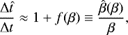
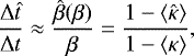
The top panel in Fig. 1 shows  as a function of β for the corresponding pairs of lensed images. We see that the time delay ratios scale remarkably well like the function
  , as predicted by Eq. (29). According to Eq. (29), the strongest effect of the SPT on time delays arises for a source as close as possible to the radial caustic, that is for β → βr. Thus, in our first example, the theoretical maximum time delay ratio equals
  for f2 = 0.5 and ν = 0.1, leading to an impact of 12% on H0. As long as it leads to a physical meaningful
  , larger (resp. smaller) values of |f2| lead to larger (resp. smaller) time delay ratios. To quantitatively evaluate the accuracy of Eq. (29), we compare the numerically evaluated quantity
  to unity, as shown in the bottom panel in Fig. 1. From Eq. (27), it follows that
  with
with  . The quantity |ηAB| is smaller than 10−4 for β ≤ 0.5 θE, reaching a maximum of |ηAB|≈ 6 × 10⁻⁴ ≪ 1 for β = 0.68 θE, confirming that εAB can be neglected in Eq. (29) in such a case. For an NIS deformed by a radial stretching characterized by Eq. (17), it is possible to derive an analytical solution for εAB, hence for |ηAB|, by solving Eq. (28). This analytical solution is represented in the bottom panel in Fig. 1 and fits perfectly the numerical evaluations of
  at each source position, as expected.
We have successfully tested the relation (29) for various axisymmetric lens profiles deformed by different deformation functions. As additional examples, we consider the two deformation functions:
 (34)
(34)
with  and f0 = −0.32, and
![Mathematical equation: \begin{equation*} f(\beta) = f_0 + \beta_0^2\,f_2\,\beta^2 \ \left[2\,\left(\beta_0^2 + \beta^2\right)\right],\end{equation*}](/articles/aa/full_html/2018/09/aa32240-17/aa32240-17-eq130.png) (35)
(35)
with β0 = 0.8 θE, f0 = −1∕3, and f2 = 1∕9. The choice for the two deformation functions (34) and (35) is justified by the fact that the resulting SPT-modified mass profiles  are approximately power laws near the tangential critical curve, that is
  (SS14). In both cases, we adopt an NIS with θc = 0.1 θE as original lens model and the same source sample as in the first example. Figure 2 shows the time delay ratios between the lensed images for each source. As expected,
  fits almost perfectly the function
  . For β = 0, the two deformation functions simplify to f(β) = f0 and the corresponding SPTs reduce to pure MSTs leading to
  and
and  , respectively. Therefore, any changes from these values reflect the impact of the SPT. For β = 0.68 θE, Fig. 2 shows an impact of around 3.6% and 2.2% on H0, respectively, which is significantly smaller than what we have obtained for the first example.
Not all combinations of SPT deformation parameters and original mass profiles κ yield a physically meaningful SPT-modified mass profile, namely  monotonically decreasing and positive definite (Schneider & Sluse 2014). In addition, the maximum time delay ratio also depends on κ since the latter directly defines the size of the radial caustic β(θr), namely the region in the source plane that produces multiple images. In summary, the way the SPT affects the time delays is very sensitive to the choice of the deformation function f, the associated deformation parameters, the original mass profile κ and lensed image positions. For these reasons, we restrain ourselves to draw generalized quantitative conclusions in the axisymmetric case. However, our numerical tests suggest an effect of a few percent in general. We will show in the next section that the simple connection between the time delay ratios and the source position ratios may still be very strong in the nonaxisymmetric case.
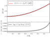 |
Fig. 1 Impact of an SPT described by the radial stretching |

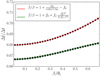 |
Fig. 2 Impact on time delays of two different SPTs defined such that the corresponding
|


4 Time delays: the nonaxisymmetric case
In this section, we drop the axisymmetry assumption for the original lens model. The SPT-modified deflection law  is thus not a curl-free field in general and there exists no deflection potential
  which satisfies
  . To define a physically meaningful modified extra light travel time, we consider the deflection law
  , the closest curl-free approximation to
  which satisfies the criterion (10) for all θ over a region
  (see Eq. (16)), and the associated deflection potential
  (see Eq. (13)). For the rest of this section, we follow USS17 and consider εacc ≈ 5 × 10⁻³ θE over the circular region |θ|≤ 2 θE, where the approximation stems from the typical positional accuracy of the Hubble Space Telescope.
Within the region  , the lensed images
  of the source
  satisfying the lens mapping
  are expected to be sufficiently close to the corresponding original images
  to not be distinguished observationally. However, we show in Sect. 4.1 that the criterion (10) defined in USS17 cannot guarantee the difference
  between the SPT-modified image position
  of the source
  and the image position θ of the source β to be smaller thanεacc over the whole region
  . However, for specific pairs of original and SPT-modified sources leading to indistinguishable image configurations, we illustrate in Sect. 4.2 the typical behavior of the time delay ratios. Finally, based solely on a numerical optimization, we slightly modify the source mapping
  by relaxing the isotropic condition of the SPT. It follows that the region where |Δ θ | < εacc can be substantially extended. From this ad hoc source mapping,
  and
and  , we illustrate the corresponding alternative time delay ratios in Sect. 4.3.
4.1 Criterion for the validity of an SPT
To illustrate the limit of the criterion |Δα(θ)| < εacc, we consider a situation similar to SS14 and USS17, namely a quadrupole lens composed of an NIS plus external shear γp (NISg) for which the deflection law is defined by
 (36)
(36)
where the core radius is set to θc = 0.1 θE. The originalsource mapping is transformed by a radial stretching (9) with a deformation function f of the form (17). The adopted SPT is thus defined by
 (37)
(37)
For the rest of this section, we set the deformation parameter f2 to be f2 = 0.4 and the external shear magnitude to be γp = 0.1. Furthermore, we exclude the effect of a pure MST by simply choosing f0 = 0. According to USS17 (see their Fig. 4), this specific pair (f2, γp) constitutes an allowed pair of parameters in a sense it fulfills the criterion |Δ α (θ)| < εacc over the circular region |θ | ≤ 2 θE. Figure 3 shows the map |Δα(θ)| over a circular grid |θ | ≤ 2 θE in the lens plane. This figure is similar to the map |Δα(θ)| illustrated in Fig. 7 in USS17, although they used f2 = 0.55. It turns out that the ratio |Δα(θi)|∕|Δα(θj)| remains unaffected when f2 varies, but is sensitive to variations of R or γp. Actually, γp is the only parameter that explicitly characterizes the degree of asymmetry of the original lens model.
The next step consists in determining how well the deflection law  allows us to reproduce the original lensed images of a source. To this aim, we create a set of mock images θ of a sample of sources β that cover the first quadrant of the source plane. We restrict the grid of sources to 0 ≤ |β|≤ 0.66 θE where multiple images are produced (see top panel in Fig. 4). Then, we produce the images
  of the corresponding SPT-modified sources
  . The bottom panel in Fig. 4 shows the image positions θ and the color-coding represents |Δθ| in units of θE. The same color-coding is applied to the sources (top panel) where only the largest offset, denoted by |Δ θ |max, are shown.
An “unexpected” conclusion can be drawn from Fig. 4; even though |Δ α (θ)| < εacc over the region |θ|≤ 2 θE (as shown in Fig. 3), many of image configurations are characterized by |Δ θ |≫ εacc for at least one lensed image. This implies that these image configurations can be distinguished from the original ones and the corresponding SPT can no longer be flagged as valid. Furthermore, the largest offsets |Δ θ | occur near the tangential critical curve. It comes with no surprise that the corresponding regions in the source plane are thus located near the tangential caustic curve. To address this behavior, we first consider what the quantity |Δ α (θ)| really represents. As defined in Eq. (10), both  and
and  are evaluated at the same position θ in the lens plane. Therefore, we have
  and
and  where
where  is the source position of the image θ under the deflection law
  . Combining the two latter equations leads to
 (38)
(38)
Equation (38) shows that minimizing |Δα(θ)| is equivalent to minimizing |Δβ| with no guarantee on |Δθ|. Indeed, let us consider a position θ close to a critical line for which |Δα(θ)| < εacc, for example (θx∕θE, θy∕θE) = (0.5, 1.0) (see Fig. 3 and bottom panel in Fig. 4). The corresponding source β (θ) is necessarily close to a caustic, so is  . Thus, the source
  lies in a region of the source plane where even small shifts |Δβ| can lead to significantly different image positions. This explains why regions where |Δ θ |≫ εacc are those which surround the critical curves. Furthermore, whereas
  is satisfied for all i ≤ j, we have
  , meaning that the θi are not lensed images of a unique source under the deflection law
  . Thus, the criterion |Δα(θi)| < εacc for a lensed image configuration θi is based upon positions that are not linked under the deflection law
  . These few simple arguments suggest with no loss of generality that the choice of Eq. (10) as a validity criterion may not be the most appropriate one.
Let us now evaluate  at the position
  instead of θ and consider the difference
  . We readily find that
 (39)
(39)
which corresponds exactly to the image shift induced by the SPT that we expect to be smaller than εacc. Assuming that  is small, we can show to first order that
 (40)
(40)
Thus, for all positions |θ|≤ 2 θE not located on a critical curve, Eq. (40) leads to
 (41)
(41)
Equation (41) clearly shows that the offsets |Δθ| are related to |Δα(θ)| through the SPT-modified Jacobi matrix  whose impact become larger as we get closer to the critical curves. Figure 5 illustrates the quantity
  using two different color-coding. The upper panel shows the same color-coding as used in Fig. 3 for comparison. It shows that a significant part of the region|θ| < 2 θE is characterized by |Δθ| > εacc even though|Δα(θ)| < εacc. The lower panel adopts a color-coding which allows us to better visualize regions characterized by the largest offsets. These regions surround the two critical curves represented by the two green lines. We confirm the validity of the first order Eq. (41) by comparing Fig. 5 with Fig. 6, which represents explicitly the quantity
  . As expected, small differences can be observed very close to the critical curves where higher order terms in Eq. (40) become significant and cannot be ignored. In addition, Fig. 6 is much more time consuming to obtain than Fig. 5. Indeed, a single
  evaluation requires
  to be calculated first, that is solving the lens equation
  that implies numerous
  evaluations. In contrast, a single Eq. (41) evaluation requires only one
  evaluation. For this reason, the grid density in bottom panel in Fig. 5 is 20 times higher than in Fig. 6.
Equation (41) confirms that the criterion |Δ α (θ)| < εacc for the validity of an SPT cannot guarantee the angular separation |Δθ| to be smaller than the astrometric accuracy of current observations, at least in regions nearby critical curves. To construct the curl-free deflection field  , USS17 have considered the action defined in Eq. (11) for which they found a minimum. This approach is based explicitly on the validity criterion (10), which is not satisfactory and should be reconsidered. A new appropriate criterion would of course imply the definition of a new action to be minimized, leading to a new definition for
  and
and  . Such a new approach is beyond the scope of this paper and will not be addressed here. Nevertheless, it remains possible to quantitatively estimate the impact of the SPT on time delays with the means available. In the next section, we first focus on the subset of source positions β depicted in the top panel in Fig. 4 that yields |Δθ| < εacc.
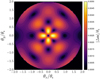 |
Fig. 3 Map of |Δα(θ)| over the circular region |θ|≤ 2 θE for f2 = 0.4, θc = 0.1 θE, and γp = 0.1. This figure issimilar to Fig. 7 in Unruh et al. (2017) with f2 = 0.55, even thoughit is based on a different approach (see the text for more details). |
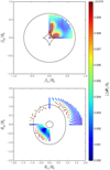 |
Fig. 4 Top panel: grid of source positions β covering the radial range 0 ≤|β|≤ 0.66 θE in the first quadrant of the source plane. Each source produces a set of lensed images θ (shown in the bottom panel) under the original deflection law α and the corresponding set of |


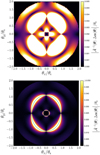 |
Fig. 5 Maps of |
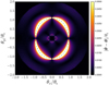 |
Fig. 6 Map of |
4.2 The SPT-modified time delays for valid configurations
In the previous section, we have shown that the criterion defined in Eq. (10) does not guarantee |Δ θ | < εacc for all |θ | ≤ 2 θE. However, the top panel in Fig. 4 also shows sources (mainly outside the tangential caustic curve) for which the corresponding largest offsets |Δθ|max between original and SPT-modified image configurations are smaller than εacc. Adopting the same original lens model as in the previous section, Fig. 7 shows the quantity
 (42)
(42)
in units of θE over the first quadrant in the source plane. The region outside the radial caustic curve is irrelevant in our case because it does not lead to multiple image configurations. The two disjointed hatched regions denoted by B1 and B2 are defined such as all sources inside B1 ∪B2 lead to image configurations characterized by |Δθ|max ≤ εacc. For f2 = 0.4 and γp = 0.1, the region B1 ∪B2 covers around 56% of the area enclosed by the radial caustic curve. Smaller values for f2 yield larger B1 ∪B2 areas, up to 100% when f2 = 0 (SPT reduced to an MST) or γp = 0 (axisymmetric lens). The regions B1 and B2 are situated on both sides of the tangential caustic curve. The very high area ratio between these two regions (1–560 in this case) indicates that most of the valid image configurations are composed of two images (the fainter third central one is always omitted). Moreover, the few valid four component configurations are very symmetric, suggesting comparable time delays between opposite image pairs.
Provided that  is physically meaningful, the curl-free deflection field
  yields indistinguishable image configurations for sources β ∈B1 ∪B2 as compared to the original α. Although these valid image configurations are of limited interest for time delay cosmography3, the resulting model ambiguities may still prevent us from performing a robust lens modeling. Thus, even though the adopted SPT is not valid over all the region |θ|≤ 2 θE, we propose in this section to analyze the time delay ratios of these particular image configurations between the original and SPT-modified models. To this aim, we consider an original nonaxisymmetric mass distribution which produces n lensed images θi of a source β ∈B1 ∪B2. The time delay Δ tij between a pair of lensed images θi and θj is defined in Eq. (3). The corresponding SPT-modified time delay
  have to be evaluated at image positions
  and
and  , respectively, leading to
![Mathematical equation: \begin{equation*} \mathrm{\Delta} \tilde{t}_{ij} = \tilde{T}\left(\tilde{\boldsymbol{\theta}}_i\right) - \tilde{T}\left(\tilde{\boldsymbol{\theta}}_j\right) = \frac{D_{\mathrm{\Delta} t}}{c} \left[\tilde{\tau}\left(\tilde{\boldsymbol{\theta}}_i\right) - \tilde{\tau}\left(\tilde{\boldsymbol{\theta}}_j\right)\right] \eqqcolon \frac{D_{\mathrm{\Delta} t}}{c} \mathrm{\Delta} \tilde{\tau}_{ij},\end{equation*}](/articles/aa/full_html/2018/09/aa32240-17/aa32240-17-eq199.png) (43)
(43)
where the SPT-modified Fermat potential is defined by
![Mathematical equation: \begin{equation*} \tilde{\tau}\left(\tilde{\boldsymbol{\theta}}\right) = \frac{1}{2} \left[ \tilde{\boldsymbol{\theta}} - \hat{\boldsymbol{\beta}}\left(\tilde{\boldsymbol{\theta}}\right) \right]^2 - \tilde{\psi}\left(\tilde{\boldsymbol{\theta}}\right) = \frac{1}{2} \left|\tilde{\boldsymbol{\alpha}}\left(\tilde{\boldsymbol{\theta}}\right)\right|^2 - \tilde{\psi}\left(\tilde{\boldsymbol{\theta}}\right).\end{equation*}](/articles/aa/full_html/2018/09/aa32240-17/aa32240-17-eq200.png) (44)
(44)
We present here the representative results obtained for two classes of models: the quadrupole NISg as defined in Eq. (36) and a non-singular isothermal elliptical lens (NIE). The NIE surface mass density κ is intrinsically nonaxisymmetric and is defined by (see e.g., Keeton 2001)
 (45)
(45)
where the variable ρ, constant on ellipses with axis ratio  , is characterized by
 (46)
(46)
For the rest of this section, the quadrupole model parameters are set to (θc, γp) = (0.1 θE, 0.1) and the NIE model parameters to (θc, ϵ) = (0.1 θE, 0.15). These models are deformed by an SPT corresponding to a radial stretching defined in Eq. (37) with f0 = 0 and f2 = 0.4. In both cases, we used pySPT to create mock images θ of two separated grids of sources β, which cover together the corresponding regions B1 ∪B2. The size and shape of B1 ∪B2 are defined by both the model and SPT parameters, hence differ from the quadrupole to the NIE (see Fig. 7 for the quadrupole and Fig. 8 for the NIE). Making use of Eq. (16), we compute the corresponding images  of the SPT-modifed sources
  . We finally derive the time delay Δtij and
  and represent their ratios in Fig. 9 (for the NISg) and Fig. 10 (for the NIE). Because of their similarities, we discuss the NISg and the NIE simultaneously.
In the double image regime, the time delay ratios scale almost like the ratios  . The color-coding in Fig. 10 refers to the azimuth angle of β, denoted as ∠β. Even though the dispersion is slightly larger for the NIE, the deviations from
  do not exceed 0.5% in all cases. The inset in Fig. 10 clearly shows that the dispersion of the time delay ratios is the effect of the relative direction of β with respect to the orientation of the axis of the elliptical iso-density contours (here equal to 0°). The deviations from
  are maximum for ∠β = 0° and ∠β = 90°, and minimum for ∠β ≈ 45°. A similar behavior is observed for the NISg, but with respect to the orientation of the external shear (also equal to 0°). We suggest that Eq. (29), valid for the axisymmetric case (see Sect. 3.1), may also be valid in the nonaxisymmetric case for sufficiently large values of |β|,
 (47)
(47)
Actually, even for the most unfavorable cases, Eq. (47) provides at least a fairly good estimate of  . It turns out that these two particular examples are representative of the time delay ratio behavior for double image configurations produced by a nonaxisymmetric lens. Thus, the impact of the SPT in the double image regime comes mainly from the ratios
  , in the same way as for the axisymmetric case. In particular, the largest time delay ratios
  (considering only the double image configurations for now) is obtained for the source position β ∈B2 characterized by the largest radial coordinate |β| and denoted as βmax. Therefore,
  depends on βmax and the latter depends on both the deformation function and the original lens model parameters, which define the size of B2. For the NISg model depicted in Fig. 9, we find
  ,
,  , leading to
  , that is an impact of around 12% on H0. For the NIE model depicted in Fig. 10, we find
  ,
,  , leading to
  , that is an impact of around 3% on H0. Similar to the axisymmetric case, the impact of the SPT on time delays may substantially vary according to the nature of the original lensmodel.
A different behavior is observed for the case of the quadruple image regime. As first pointed out in SS13 from a pure empirical case, the time delay ratios of image pairs between the original and SPT-modified models are not conserved, that is  with i < k ≤ 4. For this reason, even though only three independent time delays can be obtained from a quadruple image configurations, we represent in Figs. 9 and 10 the time delay ratios for all six image permutations (i, j) ∈ [(1, 2), (1, 3), (1, 4), (2, 3), (2, 4), (3, 4)]. We note that the criterion chosen for ordering the images (1–4) is the extra light travel time, from smallest to largest. The pair of opposite images, namely (θ1, θ2) and (θ3, θ4), leads to
  close to 1, regardless of the adopted original lens model we have tested (see the pairs of green triangles close to 1 in bottom panels in Figs. 9 and 10). Owing to the symmetry of the image configurations (B1∋ β ~ 0), the time delays Δt12 and Δt34 are smaller than the time delays between other image combinations, tending towards 0 when β approaches 0. The same holds true for the SPT-modified time delays, while we note that
  and
and  . For sources β ∈ B1, the mean impact of the SPT, denoted as
  , is around of a few percent for both the NISg and the NIE. In contrast to the NISg, the impact of the SPT for the case of the NIE is larger in the quadruple image regime than in the double image regime. This only reflects that
  while
while  .
.
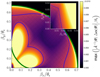 |
Fig. 7 Map of |Δθ(β)|max in units of θE for f2 = 0.4 and γp = 0.1 (see Eq. (42)). The inner (resp. outer) green line represents the tangential (resp. radial) caustic curve. The two hatched regions (B1 and B2) delimited by blue curves demarcate parts of the source plane where |Δθ(β)|max ≤ 5 × 10⁻³ θE. The region B1 lies inside the tangential caustic curve while B2 lies outside. The inset highlight the region around the position β = 0. |
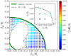 |
Fig. 8 Grid of sources β located inside the region B1 ∪B2 for the NIE with (θc, ϵ) = (0.1 θE, 0.15). The inner (resp. outer) green line represents the tangential (resp. radial) caustic curve. The color-coding refers to the offsets |Δ θ |∕θE between the lensed images θ of the sources β and the lensed images |


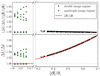 |
Fig. 9 Time delay ratios of image pairs between the NISg and the corresponding SPT-modified model. The model parameters are (θc, γp) = (0.1 θE, 0.1) and the radial stretching is characterized by f2 = 0.4. Top panel: |


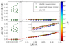 |
Fig. 10 Time delay ratios of image pairs between the NIE and the corresponding SPT-modified model. The model parameters are (θc, ϵ) = (0.1 θE, 0.15) and the radial stretching is characterized by f2 = 0.4. The time delay ratios in the quadruple (resp. double) image regime are depicted with triangles (resp. inverted triangles). The red line shows the source position ratios
|


4.3 The alternative SPT-modified time delays
In Sect. 4.1, we have shown that the capability of the deflection law  to predict the same multiple images as predicted by α (with an accuracy of εacc) is very limited (see Eq. (41)). Based upon a representative example, Fig. 7 shows that only a very small region (B1) in the source plane leads to indistinguishable quadruple image configurations. In this section, we investigate a method to extend the region in the lens plane where the offsets |Δθ| are smaller than εacc. The idea consists in finding source positions β⋆ in the vicinity of
  that lead to new image positions
 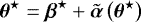 in such a way that the offsets |Δ θ ⋆||θ⋆ −θ| are as small as possible. The search for each β⋆ is based on the numerical minimization of the cost function h(β⋆) defined by
 (48)
(48)
using the Levenberg–Marquardt algorithm (Levenberg 1944). Because we expect β ⋆ to be close to the corresponding  , we always choose the latter as first guesses while we do not restrict β⋆ to share the same direction as
  . Thus, the resulting source mapping
  , hence β⋆(β), may not be isotropic as for the radial stretching.
As we shall see, this approach may drastically increase the region B1 ∪B2 (in particular B1) while benefiting from a simple implementation. However, we must point out that this method suffers several flaws. First, the source mapping β ⋆ (β) lacks a solid analytical basis. While  gives rise to
  which is analytically connected to
  by definition4, there is no apparent link between
  and β⋆. Moreover, the way it is obtained precludes any further analytical investigation. Second, there is no definitive guarantee for the source mapping β ⋆ (β) to be one-to-one over
  . Finally, a successful minimization of the cost function h for a given β⋆ does not guarantee |Δθ⋆| to be smaller than εacc. Indeed, the solution β ⋆ only corresponds to the one for which the cost function h(β⋆) is the smallest in the vicinity of
  , being potentially larger than εacc. This is particularly true for sources which are located very close to the caustic curves. At least, we have |Δ θ ⋆|≤|Δθ| where the equality holds when
  . For these reasons, we point out that this numerical approach cannot supplant the analytical reconsideration of how the curl-free deflection law
  is defined. However, the combination of β⋆(β) and
  constitutes a physically meaningful alternative to β and α, and deserves to be considered.
To illustrate the method, we adopt the same lens model and SPT as in Sect. 4.1. We also consider the same grid of sources β covering the first quadrant of the source planeand restricted to 0 ≤|β|≤ 0.66 θE. We illustrate the results of the numerical optimization in Figs. 11 and 12. The ratio |β ⋆ |∕|β| plotted against |β|∕θE in Fig. 11 clearly shows the slight anisotropy of the source mapping β ⋆ (β) resulting from the numerical optimization. Indeed, for original sources located on a quarter circle with a radius |β |, the corresponding |β ⋆ | depend on the azimuth angle ∠β; |β ⋆ | is larger than  for ∠β > 45° and smaller for ∠β < 45°. For sources leading to double image configurations, the |β⋆| scatter is around 1%. Furthermore, discontinuities in the mapping β⋆(β) appear when a source crosses the tangential caustic curve. Two particular jumps are highlighted for sources passing through the two cusps. The ones located on the βx-axis and βy-axis are explicitely depicted in Fig. 11. Due to these discontinuities, an extended source which crosses the tangential caustic curve is not mapped smoothly onto an SPT-modified extended source. This effect propagates to the image plane, but the impact on the corresponding lensed image is not observable, as shown in Fig. 12. Similar to Fig. 4, the bottom panel in Fig. 12 represents the image positions θ and the color-coding shows the offsets |Δθ⋆| in unit of θE. The same color-coding is also applied to the sources where only the largest offset between the corresponding pairs of lensed images are shown (see top panel in Fig. 12). Figure 12 shows that almost all the offsets |Δ θ ⋆| are now smaller than εacc, even for sources located inside the tangential caustic curve. It is worth stating that a finer source grid would have led to a larger number of sources located very close to the caustic curves, for which the optimized cost function may be larger than εacc. Compared to Fig. 4, some image positions depicted in Fig. 12 show an offset |Δ θ ⋆| (after the optimization process) larger than the offset |Δθ| (before the optimization process). For example, the image position θk = (1.242, 0) θE of the source β = (0.117, 0) θE is characterized by |Δθk| = 0.001 θE while
 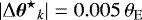 . This behavior stems from the fact that, for a given n-image configuration, the optimization process minimizes only the largest offset but not all the n offsets simultaneously (because of the max(⋅) function in Eq. (48)). Thus, while the largest offset becomes smaller, the offset
  also varies during the optimization process, leading at the end to
  .
.
Now that we have obtained a large set of indistinguishable image configurations, we derive the time delays Δ tij and  between image pairs where
  is defined by
![Mathematical equation: \begin{equation*} \mathrm{\Delta} t_{ij}^{\star} = \tilde{T}\left({\boldsymbol{\theta}^{\star}}_i\right) - \tilde{T}\left({\boldsymbol{\theta}^{\star}}_j\right) = \frac{D_{\mathrm{\Delta} t}}{c} \left[\tilde{\tau}\left({\boldsymbol{\theta}^{\star}}_i\right) - \tilde{\tau}\left({\boldsymbol{\theta}^{\star}}_j\right)\right].\end{equation*}](/articles/aa/full_html/2018/09/aa32240-17/aa32240-17-eq250.png) (49)
(49)
Figure 13 plots the time delay ratios Δt⋆∕Δt (bottom panel) and the time delay ratios normalized by |β⋆|∕|β| (top panel), both against |β|∕θE. The same color-coding as in Fig. 11 is also applied to the time delay ratios. In the double image regime, the normalized time delay ratios (Δt⋆∕Δt)∕(|β⋆|∕|β|) is close to 1. This suggests once again that the time delay ratios scale almost like the source ratios |β ⋆ |∕|β|, even though the source mapping is not perfectly isotropic. Thus, the equation
 (50)
(50)
still holds for the slight anisotropic source mapping β⋆(β) and is particularly true for large |β| inside the radial caustic curve. In the quadruple image regime, the time delay ratios of image pairs between the models are also not perfectly conserved. In either panels in Fig. 13, we represent the mean between the six time delay ratios and the corresponding standard deviation, denoted as σ(Δ t⋆∕Δt) and depicted with error bars. However, σ(Δt⋆∕Δt) is around a minimum of 0.001 for ∠β = 0° when β points towards the same direction as the external shear. Conversely, it reaches a maximum of 0.02 for ∠β = 90° when β points perpendicularly to the direction of the external shear. In addition for ∠β = 0°, the time delay ratios Δt⋆∕Δt scale like |β ⋆ |∕|β|, regardless of the image combinations. Thus, as the azimuth angle ∠β increases, the time delay ratios Δt⋆∕Δt deviates from |β⋆|∕|β| and the corresponding σ(Δt⋆∕Δt) also increases. We recall that prior to any numerical optimization, the time delays ratios  were close to 1 only for pairs of opposite images. Quantitatively, the impact of the SPT on the time delays agrees with what we have obtained in Figs. 9 and 10, that is an impact of a few percent. It turns out that most of the conclusions drawn in Sect. 4.2 seem to apply in this case as well.
In Sect. 4.1 we suggest to reconsider the criterion for the validity of an SPT as formulated in Unruh et al. (2017). This shall lead to more appropriate definition of the SPT-transformed deflection law and potential, enlarging the scope where the SPT is a valid invariance transformation. Because Eq. (50) holds within the numerical approach described inthis section, we expect that Eq. (47) will also remain true when considering new definitions for  and
and  , and an isotropic SPT. Thus, most of the conclusions drawn in this paper should remain unchanged.
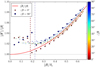 |
Fig. 11 Ratios |β⋆|∕|β| plotted against β in units of θE. The source positions β⋆ are obtained by means of a numerical optimization of the cost function h(β⋆) defined in Eq. (48). The resulting source mapping β⋆(β) is slightly anisotropic: |β⋆| is larger than |

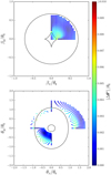 |
Fig. 12 Bottom panel: set of mock lensed images θ produced by the source positions shown in the top panel and lensed by an NIS plus external shear characterized by θc = 0.1 θE and γp = 0.1. The color-coding represents the image offsets |Δθ⋆| in units of θE between θ and θ ⋆. The latter are the images of the source positions β⋆ that are lensed by the SPT-modified lens associated with |


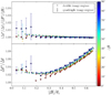 |
Fig. 13 Time delay ratios of image pairs between the NISg and the corresponding SPT-modified model associated with the curl-free deflection field |


5 Conclusions
The SPT corresponds to a global invariance transformation of the source plane. It gives rise to a new deflection law, which leaves almost all the lensing observables invariant. We have studied the impact of the SPT on the time delays between pairs of lensed images produced by both axisymmetric and nonaxisymmetric lenses. Although we have mainly considered the case of an isotropic SPT described by a radial stretching of the form ![Mathematical equation: $\hat{\boldsymbol{\beta}} = [1 + f(|\boldsymbol{\beta}|)]\,\boldsymbol{\beta}$](/articles/aa/full_html/2018/09/aa32240-17/aa32240-17-eq255.png) , we have also addressed a particular case for which the STP is slightly anisotropic.
, we have also addressed a particular case for which the STP is slightly anisotropic.
Owing to its simplicity, we were able to deal with the axisymmetric case in an analytical way. We have shown that the time delay ratios of image pairs between the SPT-modified and original models approximate as the ratios between the SPT-modified and original source positions, namely 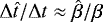 . Based on simple analytical arguments, we have demonstrated that this relation holds for any axisymmetric lenses and even deformation function f. In particular, this relation is exact when the SPT reduces to an MST or when the lens is described by an SIS model, regardless of the deformation function f. For an NIS model deformed by a radial stretching of the form
 ![Mathematical equation: $\hat{\beta}(\beta) = [1 + f_2\,\beta^2 / (2\,\theta_{\rm{{E}}}^2)]\,\beta$](/articles/aa/full_html/2018/09/aa32240-17/aa32240-17-eq257.png) , we have shown that
, we have shown that  deviates no more than a few hundredth of percent from
  . In addition, we have demonstrated that the source mapping can be expressed in terms of the mean surface mass densities, that is
 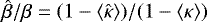 .
.
Quantitatively, the impact of the SPT on time delays may reach a few percent for particular image configurations, and depends on various factors. Indeed,  depends on the choice made for the deformation function f and its corresponding deformation parameters. Not all combinations of an original mass profile κ, a function f, and a set of deformation parameters yield a physically meaningful SPT-modified mass profile
  . It means that the parameter validity range of a given SPT, hence the validity range of
  or
or  , needs to be studied on a case-by-case basis.
When we drop the axisymmetry assumption for the original lens model, the SPT-modified deflection angle  is not a curl-free field caused by a mass distribution corresponding to a gravitational lens (SS14). An alternative deflection field
  was proposed in USS17, namely the closest curl-free approximation to
  which fulfills the validity criterion
  over a region
  in the lens plane where multiple images occur. We have studied in detail the relevance of this criterion using εacc = 5 × 10⁻³ θE as suggested in USS17. We have shown that this criterion is not appropriate, in particular for positions close to the critical lines. Indeed, we have demonstrated to first order that the offsets |Δ θ | between the original and SPT-modified lensed images depends on the SPT-modified Jacobi matrix whose impact become larger as we get closer to the critical curves,
 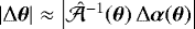 . Thus, the criterion |Δα(θ)|≤ εacc over
  does not guarantee the image offsets |Δθ| to be smaller than εacc over the same region. In those cases, the deflection field
  produces image configurations which can be observationally distinguished from the original ones. As a result, we suggest that the criterion |Δα(θ)|≤ εacc proposed in USS17 should be reconsidered, which also means a revision of how the curl-free deflection law
  and
and  are defined.
For the indistinguishable image configurations produced by  , we have studied how the time delays are affected by the SPT. For a quadrupole (NIS + shear) and a NIE models, we have shown that, once again, the time delay ratios scale like the source position ratios, i.e.
  , when two images are produced. This result holds for opposite image pairs when four images are produced. For other image pair combinations, we confirm that the time delay ratios are not conserved. Thus, accurate time delay ratios measurements should help to reduce the degeneracy between SPT-generated models. However, the impact of the SPT remains low with deviations not larger than a few percent for the illustrative examples we have considered.
To extend the range of indistinguishable image configurations produced by  , we have slightly modified the source mapping by means of a numerical optimization,
  . We tested this method on a quadrupole model (NIS + shear) deformed by a radial stretching. The new source mapping differs from a radial stretching in the sense that β⋆(β) is slightly anisotropic and shows discontinuities when a source crosses the tangential caustic curve. In the same way as for the previous cases, the time delay ratios of image pairs scale like the source position ratios, i.e. Δ t⋆ ∕Δt ≈|β⋆|∕|β|, when two images are produced. When four images are produced, the time delay ratios are sensitive to the azimuth angle of β. We have shown that they scale like the source position ratios when the azimuth angle is parallel to the external shear direction and deviate to a few percent when the azimuth angle is perpendicular to the external shear direction. As a general conclusion, the impact of the SPT on time delay cosmography seems not be as crucial as initially suspected, leading to deviations that do not exceed a few percent.
In a future work, we aim to reconsider the validity criterion in more detail by redefining the curl-free deflection field  and the corresponding potential
  . Although new definitions for
  and
and  will affect the time delays, we expect that it will not modify substantially the results presented in this paper, likely leaving most of the conclusions unchanged.
Acknowledgements
We thank Dominique Sluse and Sandra Unruh for useful discussions. This work was supported by the Humboldt Research Fellowship for Postdoctoral Researchers.
Appendix A Proof that εAB = 0 for an SIS and a radial stretching of the form (eqnlinking 19)
For the sake of clarity, we first recall the definition of εAB given in Eq. (28):
![Mathematical equation: \begin{equation*} {\varepsilon}_{\textrm{AB}} = \int_{|\theta_{\rm{{B}}}|}^{\theta_{\rm{{A}}}} \beta(\theta) \left[f(\beta(\theta)) - f(\beta_{\text{s}})\right]\ \text{d}\theta \ .\vspace*{-4pt}\end{equation*}](/articles/aa/full_html/2018/09/aa32240-17/aa32240-17-eq283.png) (A.1)
(A.1)
In this section, we will proof that εAB = 0 for an SIS and for any deformation function f(β) which satisfies a few reasonable conditions. By definition, f(β) must be even to preserve the symmetry and 1 + f(β) + β df(β)∕dβ > 0 guarantees the mapping to be one-to-one. Let us assume that f(β) is a real analytic function, its Maclaurin series expansion thus exists and is simply given by
 (A.2)
(A.2)
where fn := dnf∕dβn is evaluated in β = 0 and f2k+1 = 0 for all  to preserve the symmetry. Because of the linearity of integration and recalling the lens equation β(θ) = θ − θEθ∕|θ| for an SIS, Eq. (A.1) transforms into
 (A.3)
(A.3)
where n is now a positive even integer or 0. Keeping in mind that n + 2 is even, the linearity of the integrand guarantees that
![Mathematical equation: \begin{equation*} \int_{|\theta_{\rm{{B}}}|}^{\theta_{\rm{{A}}}} (\theta - \theta_{\rm{{E}}})^{n+1}\ \text{d}\theta = \left[ \frac{(\theta - \theta_{\rm{{E}}})^{n+2}}{n+2} \right]_{|\theta_{\rm{{B}}}|}^{\theta_{\rm{{A}}}} = 0 \ ,\vspace*{-4pt}\end{equation*}](/articles/aa/full_html/2018/09/aa32240-17/aa32240-17-eq287.png) (A.4)
(A.4)
where in the last step we used θA − θE = βs and |θB |− θE = −βs. Because the latter expression is valid for all positive even integer n and for n = 0, we deduce that all the successive terms in the series vanish, as the second integral in Eq. (A.3), leading to εAB = 0. Furthermore, the accuracy of (A.2) is not affected by the value at which the function is evaluated as long as the series converges. Thus, we finally require that the radius of convergence r of the Maclaurin series (A.2) satisfies the condition r ≥ θE. If satisfied, this very plausible assumption ensures the series expansion (A.2) to be exact for all β <θE.
Appendix B Proof that εAB ≈ 0 for any axisymmetric model and radial stretching of the form (eqnlinking 19)
To convince the reader, we consider separately the cases when βs tends to 0 (βs → 0) and when βs < β(θr), where θr corresponds to the angular radius of the radial critical curve.
For βs → 0, we see from Eq. (28) that the integration interval degenerates into {θt}, where θt corresponds to the angular radius of the tangential critical curve. Thus, the integrand also tends to 0 and εAB → 0. In addition, εAB → 0 faster than Δ τAB → 0 due to the first term in Eq. (26) while 1 + f(βs) → 1. Thus, we deduce that the εAB-term in Eq. (27) can be neglected when βs → 0.
For βs < β(θr), we define the quantity
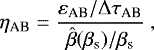 (B.1)
(B.1)
and show that |ηAB|≪ 1, which is sufficient to guarantee that the εAB-term in Eq. (27) can be neglected. With this aim in mind, we analyze the graph of the integrand ![Mathematical equation: $\beta(\theta) \left[f(\beta(\theta)) - f(\beta_{\text{s}})\right] \eqqcolon \beta(\theta) F(\beta(\theta))$](/articles/aa/full_html/2018/09/aa32240-17/aa32240-17-eq289.png) defined in Eq. (28) and for which an example is shown in Fig. B.1. Based on general considerations, we expect the graph of the integrand to be almost symmetric with respect to the point (θt, 0) over the interval [|θB |, θA]. First, the graph of β(θ) monotonically increases over [|θB|, θA] and always crosses the θ-axis at the position θ = θt ≈ (θA + |θB|)∕2. These statements stem from the general properties of axisymmetric lenses in the case of a single lens plane (see e.g. Sect. 3.1 in Schneider 2006). In addition, because of dβ(θ)∕dθ is almost constant (≈1) for most θ ∈ [|θB|, θA], the graph of β(θ) is almost symmetric with respect to the point (θt, 0). The largest asymmetry occurs for βs → β(θr) for which |θB|→ θr (this “unfavorable” case is actually the one shown in Fig. B.1). Second, the graph of F(β(θ)) can only cross the θ-axis at the positions θA and θB over [|θB |, θA], and is almost symmetric with respect to the axis θ = θt. We easily confirm that θA and θB are θ-intercepts from F(β(θA)) = F(β(θB)) = F(βs) = 0. To show there exists no other θ-intercept within [|θB |, θA], we use a reduction ad absurdum argument. If the graph of F(β(θ)) crosses the θ-axis at a third position θI ∈ [|θB|, θA], then F(β(θI)) = 0 implies that θI corresponds to the position of a lensed image of the source βs. Since the third image θC always satisfies the condition 0 < |θC| < |θB| < θI < θA, hence θC∉[|θB|, θA], the existence of this fourth lensed image violates the so-called “odd number theorem” (Dyer & Roeder 1980; Burke 1981) in the case of a single lens plane. In addition, because of the symmetry of β(θ) for θ ∈ [|θB|, θA] and recalling that f is an even function of β, we have F(β(θt + δθ)) ≈ F(β(θt − δθ)), with δθ ∈ [0, min(θA − θt, θt −|θB|)], which guarantees F(β(θ)) to be almost symmetric with respectto the axis θ = θt. Combining all these statements leads to the conclusion that the integrand β(θ)F(β(θ)) is also almost symmetric with respectto (θt, 0). Thus, the integral (28) consists in differencing the (almost identical) gray areas displayed inFig. B.1, which tends to compensate each other, leading to |εAB|≪ θt. Finally, from Eq. (26) we deduce that |ΔτAB|≈ 2 βs θt due to the symmetry of β(θ) over [|θB |, θA]. As a conclusion, we find |ηAB|≪ 1 from Eq. (B.1), which confirms that the εAB term in Eq. (27) can be in general neglected.
defined in Eq. (28) and for which an example is shown in Fig. B.1. Based on general considerations, we expect the graph of the integrand to be almost symmetric with respect to the point (θt, 0) over the interval [|θB |, θA]. First, the graph of β(θ) monotonically increases over [|θB|, θA] and always crosses the θ-axis at the position θ = θt ≈ (θA + |θB|)∕2. These statements stem from the general properties of axisymmetric lenses in the case of a single lens plane (see e.g. Sect. 3.1 in Schneider 2006). In addition, because of dβ(θ)∕dθ is almost constant (≈1) for most θ ∈ [|θB|, θA], the graph of β(θ) is almost symmetric with respect to the point (θt, 0). The largest asymmetry occurs for βs → β(θr) for which |θB|→ θr (this “unfavorable” case is actually the one shown in Fig. B.1). Second, the graph of F(β(θ)) can only cross the θ-axis at the positions θA and θB over [|θB |, θA], and is almost symmetric with respect to the axis θ = θt. We easily confirm that θA and θB are θ-intercepts from F(β(θA)) = F(β(θB)) = F(βs) = 0. To show there exists no other θ-intercept within [|θB |, θA], we use a reduction ad absurdum argument. If the graph of F(β(θ)) crosses the θ-axis at a third position θI ∈ [|θB|, θA], then F(β(θI)) = 0 implies that θI corresponds to the position of a lensed image of the source βs. Since the third image θC always satisfies the condition 0 < |θC| < |θB| < θI < θA, hence θC∉[|θB|, θA], the existence of this fourth lensed image violates the so-called “odd number theorem” (Dyer & Roeder 1980; Burke 1981) in the case of a single lens plane. In addition, because of the symmetry of β(θ) for θ ∈ [|θB|, θA] and recalling that f is an even function of β, we have F(β(θt + δθ)) ≈ F(β(θt − δθ)), with δθ ∈ [0, min(θA − θt, θt −|θB|)], which guarantees F(β(θ)) to be almost symmetric with respectto the axis θ = θt. Combining all these statements leads to the conclusion that the integrand β(θ)F(β(θ)) is also almost symmetric with respectto (θt, 0). Thus, the integral (28) consists in differencing the (almost identical) gray areas displayed inFig. B.1, which tends to compensate each other, leading to |εAB|≪ θt. Finally, from Eq. (26) we deduce that |ΔτAB|≈ 2 βs θt due to the symmetry of β(θ) over [|θB |, θA]. As a conclusion, we find |ηAB|≪ 1 from Eq. (B.1), which confirms that the εAB term in Eq. (27) can be in general neglected.
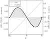 |
Fig. B.1 Graph of the integrand β(θ)F(β(θ)) (thick black curve) defined in Eq. (28) for the “unfavorable” case |θB | → θr. This integrand is composed of the functions β(θ) (solid gray curve) and F(β(θ)) (dashed graycurve). The (almost) symmetrical graph of β(θ) with respect to (θt, 0) and F(β(θ)) with respect to the axis θ = θt (dotted vertical line) implies the (almost) symmetry of the integrand with respect to (θt, 0). As a consequence, the two gray areas (almost) compensate each other implying that |εAB | ≪ θt, hence |ηAB|≪ 1, and confirms the validity of the Eq. (29). |
References
- Akhunov, T. A., Wertz, O., Elyiv, A., et al. 2017, MNRAS, 465, 3607 [NASA ADS] [CrossRef] [Google Scholar]
- Bar-Kana, R. 1996, ApJ, 468, 17 [NASA ADS] [CrossRef] [Google Scholar]
- Birrer, S., Amara, A., & Refregier, A. 2016, JCAP, 8, 020 [NASA ADS] [CrossRef] [Google Scholar]
- Blandford, R. D., & Narayan, R. 1992, ARA&A, 30, 311 [NASA ADS] [CrossRef] [Google Scholar]
- Bonvin, V., Courbin, F., Suyu, S. H., et al. 2017, MNRAS, 465, 4914 [NASA ADS] [CrossRef] [Google Scholar]
- Burke, W. L. 1981, ApJ, 244, L1 [NASA ADS] [CrossRef] [Google Scholar]
- Coe, D., & Moustakas, L. A. 2009, ApJ, 706, 45 [NASA ADS] [CrossRef] [Google Scholar]
- Courbin, F., Chantry, V., Revaz, Y., et al. 2011, A&A, 536, A53 [NASA ADS] [CrossRef] [EDP Sciences] [Google Scholar]
- Dyer, C. C., & Roeder, R. C. 1980, ApJ, 238, L67 [NASA ADS] [CrossRef] [Google Scholar]
- Eulaers, E., Tewes, M., Magain, P., et al. 2013, A&A, 553, A121 [NASA ADS] [CrossRef] [EDP Sciences] [Google Scholar]
- Falco, E. E., Gorenstein, M. V., & Shapiro, I. I. 1985, ApJ, 289, L1 [Google Scholar]
- Fassnacht, C. D., Gal, R. R., Lubin, L. M., et al. 2006, ApJ, 642, 30 [NASA ADS] [CrossRef] [Google Scholar]
- Finet, F., & Surdej, J. 2016, A&A, 590, A42 [NASA ADS] [CrossRef] [EDP Sciences] [Google Scholar]
- Finet, F., Elyiv, A., & Surdej, J. 2012, Mem. Soc. Astron. It., 83, 944 [NASA ADS] [Google Scholar]
- Finet, F., Elyiv, A., Melnyk, O., et al. 2015, MNRAS, 452, 1480 [NASA ADS] [CrossRef] [Google Scholar]
- Fohlmeister, J., Kochanek, C. S., Falco, E. E., et al. 2013, ApJ, 764, 186 [NASA ADS] [CrossRef] [Google Scholar]
- Gorenstein, M. V., Shapiro, I. I., & Falco, E. E. 1988, ApJ, 327, 693 [NASA ADS] [CrossRef] [Google Scholar]
- Jean, C., Claeskens, J.-F., & Surdej, J. 2001, ASP Conf. Ser., 237, 423 [Google Scholar]
- Keeton, C. R. 2001, ArXiv e-prints [arXiv:astro-ph/0102341] [Google Scholar]
- Keeton, C. R. 2003, ApJ, 584, 664 [NASA ADS] [CrossRef] [Google Scholar]
- Kochanek, C. S. 2002, ApJ, 578, 25 [NASA ADS] [CrossRef] [Google Scholar]
- Kochanek, C. S. 2006, in Gravitational Lensing: Strong, Weak and Micro, Saas-Fee Advanced Course 33, eds. G. Meylan, et al. (Berlin: Springer), 91 [Google Scholar]
- Koopmans, L. V. E., Treu, T., Fassnacht, C. D., Blandford, R. D., & Surpi, G. 2003, ApJ, 599, 70 [NASA ADS] [CrossRef] [Google Scholar]
- Levenberg, K. 1944, Quart. J Appl. Math., 2, 164 [Google Scholar]
- Liao, K., Treu, T., Marshall, P., et al. 2015, ApJ, 800, 11 [NASA ADS] [CrossRef] [Google Scholar]
- Liesenborgs, J., & De Rijcke S. 2012, MNRAS, 425, 1772 [NASA ADS] [CrossRef] [Google Scholar]
- McCully, C., Keeton, C. R., Wong, K. C., & Zabludoff, A. I. 2014, MNRAS, 443, 3631 [NASA ADS] [CrossRef] [Google Scholar]
- McCully, C., Keeton, C. R., Wong, K. C., & Zabludoff, A. I. 2016, AAS Meeting Abstracts, 227, 338.02 [Google Scholar]
- Oguri, M., & Marshall, P. J. 2010, MNRAS, 405, 2579 [NASA ADS] [Google Scholar]
- Paraficz, D., & Hjorth, J. 2010, ApJ, 712, 1378 [NASA ADS] [CrossRef] [Google Scholar]
- Rathna Kumar, S., Tewes, M., Stalin, C. S., et al. 2013, A&A, 557, A44 [NASA ADS] [CrossRef] [EDP Sciences] [Google Scholar]
- Refsdal, S. 1964, MNRAS, 128, 307 [NASA ADS] [CrossRef] [Google Scholar]
- Saha, P. 2000, AJ, 120, 1654 [NASA ADS] [CrossRef] [Google Scholar]
- Schneider, P. 2006, in Gravitational Lensing: Strong, Weak and Micro, Saas-Fee Advanced Course 33, eds. G. Meylan, et al. (Berlin: Springer), 1 [Google Scholar]
- Schneider, P. 2014a, A&A, 568, L2 [NASA ADS] [CrossRef] [EDP Sciences] [Google Scholar]
- Schneider, P. 2014b, A&A, submitted [arXiv:1409.0015] [Google Scholar]
- Schneider, P., & Sluse, D. 2013, A&A, 559, A37 [NASA ADS] [CrossRef] [EDP Sciences] [Google Scholar]
- Schneider, P., & Sluse, D. 2014, A&A, 564, A103 [NASA ADS] [CrossRef] [EDP Sciences] [Google Scholar]
- Seljak, U. 1994, ApJ, 436, 509 [NASA ADS] [CrossRef] [Google Scholar]
- Suyu, S. H., Marshall, P. J., Auger, M. W., et al. 2010, ApJ, 711, 201 [NASA ADS] [CrossRef] [Google Scholar]
- Suyu, S. H., Auger, M. W., Hilbert, S., et al. 2013, ApJ, 766, 70 [NASA ADS] [CrossRef] [Google Scholar]
- Tewes, M., Courbin, F., Meylan, G., et al. 2013, A&A, 556, A22 [NASA ADS] [CrossRef] [EDP Sciences] [Google Scholar]
- Treu, T., & Marshall, P. J. 2016, A&ARv, 24, 11 [Google Scholar]
- Unruh, S., Schneider, P., & Sluse, D. 2017, A&A, 601, A77 [NASA ADS] [CrossRef] [EDP Sciences] [Google Scholar]
- Vuissoz, C., Courbin, F., Sluse, D., et al. 2008, A&A, 488, 481 [NASA ADS] [CrossRef] [EDP Sciences] [Google Scholar]
- Wertz, O., & Orthen, B. 2018, ArXiv e-prints [arXiv:1801.04151] [Google Scholar]
- Wong, K. C., Keeton, C. R., Williams, K. A., Momcheva, I. G., & Zabludoff, A. I. 2011, ApJ, 726, 84 [NASA ADS] [CrossRef] [Google Scholar]
- Wong, K. C., Suyu, S. H., Auger, M. W., et al. 2017, MNRAS, 465, 4895 [NASA ADS] [CrossRef] [Google Scholar]
- Wucknitz, O. 2002, MNRAS, 332, 951 [NASA ADS] [CrossRef] [Google Scholar]
- Xu, D., Sluse, D., Schneider, P., et al. 2016, MNRAS, 456, 739 [NASA ADS] [CrossRef] [Google Scholar]
We note that the time delay distance  inferred from a model that neglects the impact of κext is related to the true time delay distance by
 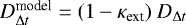 .
.
The inner lensed image is most of the time not observed.
The sources located inside the region B1 produce very symmetric quadruply imaged configurations, while those located inside the region B2 produce only doubled image configurations. In both cases, only one relevant time delay can be inferred from these systems.
We also recall the analytical relation  over
over  .
.
All Figures
|
Fig. 1 Impact of an SPT described by the radial stretching |
| In the text | |
|
Fig. 2 Impact on time delays of two different SPTs defined such that the corresponding
|
| In the text | |
|
Fig. 3 Map of |Δα(θ)| over the circular region |θ|≤ 2 θE for f2 = 0.4, θc = 0.1 θE, and γp = 0.1. This figure issimilar to Fig. 7 in Unruh et al. (2017) with f2 = 0.55, even thoughit is based on a different approach (see the text for more details). |
| In the text | |
|
Fig. 4 Top panel: grid of source positions β covering the radial range 0 ≤|β|≤ 0.66 θE in the first quadrant of the source plane. Each source produces a set of lensed images θ (shown in the bottom panel) under the original deflection law α and the corresponding set of |
| In the text | |
|
Fig. 5 Maps of |
| In the text | |
|
Fig. 6 Map of |
| In the text | |
|
Fig. 7 Map of |Δθ(β)|max in units of θE for f2 = 0.4 and γp = 0.1 (see Eq. (42)). The inner (resp. outer) green line represents the tangential (resp. radial) caustic curve. The two hatched regions (B1 and B2) delimited by blue curves demarcate parts of the source plane where |Δθ(β)|max ≤ 5 × 10⁻³ θE. The region B1 lies inside the tangential caustic curve while B2 lies outside. The inset highlight the region around the position β = 0. |
| In the text | |
|
Fig. 8 Grid of sources β located inside the region B1 ∪B2 for the NIE with (θc, ϵ) = (0.1 θE, 0.15). The inner (resp. outer) green line represents the tangential (resp. radial) caustic curve. The color-coding refers to the offsets |Δ θ |∕θE between the lensed images θ of the sources β and the lensed images |
| In the text | |
|
Fig. 9 Time delay ratios of image pairs between the NISg and the corresponding SPT-modified model. The model parameters are (θc, γp) = (0.1 θE, 0.1) and the radial stretching is characterized by f2 = 0.4. Top panel: |
| In the text | |
|
Fig. 10 Time delay ratios of image pairs between the NIE and the corresponding SPT-modified model. The model parameters are (θc, ϵ) = (0.1 θE, 0.15) and the radial stretching is characterized by f2 = 0.4. The time delay ratios in the quadruple (resp. double) image regime are depicted with triangles (resp. inverted triangles). The red line shows the source position ratios
|
| In the text | |
|
Fig. 11 Ratios |β⋆|∕|β| plotted against β in units of θE. The source positions β⋆ are obtained by means of a numerical optimization of the cost function h(β⋆) defined in Eq. (48). The resulting source mapping β⋆(β) is slightly anisotropic: |β⋆| is larger than |
| In the text | |
|
Fig. 12 Bottom panel: set of mock lensed images θ produced by the source positions shown in the top panel and lensed by an NIS plus external shear characterized by θc = 0.1 θE and γp = 0.1. The color-coding represents the image offsets |Δθ⋆| in units of θE between θ and θ ⋆. The latter are the images of the source positions β⋆ that are lensed by the SPT-modified lens associated with |
| In the text | |
|
Fig. 13 Time delay ratios of image pairs between the NISg and the corresponding SPT-modified model associated with the curl-free deflection field |
| In the text | |
|
Fig. B.1 Graph of the integrand β(θ)F(β(θ)) (thick black curve) defined in Eq. (28) for the “unfavorable” case |θB | → θr. This integrand is composed of the functions β(θ) (solid gray curve) and F(β(θ)) (dashed graycurve). The (almost) symmetrical graph of β(θ) with respect to (θt, 0) and F(β(θ)) with respect to the axis θ = θt (dotted vertical line) implies the (almost) symmetry of the integrand with respect to (θt, 0). As a consequence, the two gray areas (almost) compensate each other implying that |εAB | ≪ θt, hence |ηAB|≪ 1, and confirms the validity of the Eq. (29). |
| In the text | |
Current usage metrics show cumulative count of Article Views (full-text article views including HTML views, PDF and ePub downloads, according to the available data) and Abstracts Views on Vision4Press platform.
Data correspond to usage on the plateform after 2015. The current usage metrics is available 48-96 hours after online publication and is updated daily on week days.
Initial download of the metrics may take a while.