| Issue |
A&A
Volume 642, October 2020
|
|
|---|---|---|
| Article Number | A119 | |
| Number of page(s) | 12 | |
| Section | Stellar structure and evolution | |
| DOI | https://doi.org/10.1051/0004-6361/202038383 | |
| Published online | 12 October 2020 | |
Disk Evolution Study Through Imaging of Nearby Young Stars (DESTINYS): A close low-mass companion to ET Cha⋆
1
Anton Pannekoek Institute for Astronomy, University of Amsterdam, Science Park 904, 1098 XH Amsterdam, The Netherlands
e-mail: This email address is being protected from spambots. You need JavaScript enabled to view it.
2
Leiden Observatory, Leiden University, PO Box 9513, 2300 RA Leiden, The Netherlands
3
Univ. Grenoble Alpes, CNRS, IPAG, 38000 Grenoble, France
4
Kapteyn Astronomical Institute, University of Groningen, PO Box 800, 9700 AV Groningen, The Netherlands
5
Jet Propulsion Laboratory, California Institute of Technology, M/S 321-100, 4800 Oak Grove Drive, Pasadena, CA 91109, USA
6
Department of Physics & Astronomy, University of Rochester, 500 Wilson Blvd., Rochester, NY 14627, USA
7
European Southern Observatory (ESO), Alonso de Córdova 3107, Vitacura, Casilla 19001, Santiago de Chile, Chile
8
Unidad Mixta Internacional Franco-Chilena de Astronomía, CNRS, UMI 3386 and Departamento de Astronomía, Universidad de Chile, Camino El Observatorio 1515, Las Condes, Santiago, Chile
9
Univ. Grenoble Alpes, CNRS, IPAG, 38000 Grenoble, France
10
European Southern Observatory, Karl-Schwarzschild-Strasse 2, 85748 Garching bei München, Germany
11
Max Planck Institute for Astronomy, Königstuhl 17, 69117 Heidelberg, Germany
12
University Observatory, Faculty of Physics, Ludwig-Maximilians-Universität München, Scheinerstr. 1, 81679 Munich, Germany
13
Exzellenzcluster ORIGINS, Boltzmannstr. 2, 85748 Garching, Germany
14
INAF, Osservatorio Astrofisico di Arcetri, Largo Enrico Fermi 5, 50125 Firenze, Italy
15
INAF-Osservatorio Astronomico di Padova, Vicolodell’Osservatorio 5, 35122 Padova, Italy
16
Harvard-Smithsonian Center for Astrophysics, Cambridge, MA 02138, USA
17
CRAL, UMR 5574, CNRS, Université de Lyon, École Normale Supérieure de Lyon, 46 Allée d’Italie, 69364 Lyon Cedex 07, France
18
School of Physics and Astronomy, Monash University, Clayton, VIC 3800, Australia
19
Hamburger Sternwarte, Gojenbergsweg 112, 21029 Hamburg, Germany
20
SRON Netherlands Institute for Space Research, Sorbonnelaan 2, 3584 CA Utrecht, The Netherlands
21
Institute for Astronomy, University of Hawai’i at Mānoa, Honolulu, HI 96822, USA
22
Facultad de Ingeniería y Ciencias, Universidad Diego Portales, Av. Ejercito 441, Santiago, Chile
Received:
8
May
2020
Accepted:
9
July
2020
Abstract
Context. To understand the formation of planetary systems, it is important to understand the initial conditions of planet formation, that is, the young gas-rich planet forming disks. Spatially resolved, high-contrast observations are of particular interest since substructures in disks that are linked to planet formation can be detected. In addition, we have the opportunity to reveal close companions or even planets in formation that are embedded in the disk.
Aims. In this study, we present the first results of the Disk Evolution Study Through Imaging of Nearby Young Stars (DESTINYS), an ESO/SPHERE large program that is aimed at studying disk evolution in scattered light, mainly focusing on a sample of low-mass stars (< 1 M⊙) in nearby (∼200 pc) star-forming regions. In this particular study, we present observations of the ET Cha (RECX 15) system, a nearby “old” classical T Tauri star (5−8 Myr, ∼100 pc), which is still strongly accreting.
Methods. We used SPHERE/IRDIS in the H-band polarimetric imaging mode to obtain high spatial resolution and high-contrast images of the ET Cha system to search for scattered light from the circumstellar disk as well as thermal emission from close companions. We additionally employed VLT/NACO total intensity archival data of the system taken in 2003.
Results. Here, we report the discovery, using SPHERE/IRDIS, of a low-mass (sub)stellar companion to the η Cha cluster member ET Cha. We estimate the mass of this new companion based on photometry. Depending on the system age, it is either a 5 Myr, 50 MJup brown dwarf or an 8 Myr, 0.10 M⊙ M-type, pre-main-sequence star. We explore possible orbital solutions and discuss the recent dynamic history of the system.
Conclusions. Independent of the precise companion mass, we find that the presence of the companion likely explains the small size of the disk around ET Cha. The small separation of the binary pair indicates that the disk around the primary component is likely clearing from the outside in, which explains the high accretion rate of the system.
Key words: binaries: close / protoplanetary disks / brown dwarfs / stars: individual: ETCha / techniques: high angular resolution / techniques: polarimetric
Based on data obtained in ESO programs 1104.C-0415(E) and 70.C-0286(A).
© ESO 2020
1. Introduction
Gas giants are formed when the circumstellar disks around young stars are still rich in gas and dust. The dust in these disks must go through a very intense and rapid phase of growth to transform particles similar in nature to the interstellar medium (ISM), which are sub-micron in size, into large bodies thousands of kilometer across. Irrespective of the exact details of this process, the formation of planets is intimately intertwined with the evolution of disks (see Morbidelli & Raymond 2016 for a recent review).
The results of surveys aimed at measuring the bulk properties and evolution timescales of disks indicate that disks around T Tauri stars dissipate on a typical timescale of 3 Myr (e.g., Haisch et al. 2001; Hernández et al. 2007; Fedele et al. 2010). They also indicate that the mass available in solids (as estimated from mm-continuum observations) is, at best, of a few Mjup by 1−2 Myr (Ansdell et al. 2016; Pascucci et al. 2016). Assuming a typical gas-to-dust mass ratio of 100, the typical total disk mass is on the order of 0.5% of the central star mass (Andrews et al. 2013). These results, along with the short timescales and limited mass involved, place stringent constraints on the planet formation mechanisms (Greaves & Rice 2010; Najita & Kenyon 2014; Manara et al. 2018).
New instruments that provide high angular resolution and high-contrast offer a new window into resolving the disks and directly study the presence and interaction of forming planets with their parental disks. However, at least for now, the results from these surveys are mostly relevant either for the brighter end of the young star sample when adaptive optics is used or to the largest and most massive disks when mm-interferometry is used (see e.g., Andrews et al. 2018; Garufi et al. 2018). In this paper, we report the first results of the Disk Evolution Study Through Imaging of Nearby Young Stars (DESTINYS), a large program carried out with SPHERE (Beuzit et al. 2019) at the ESO/VLT. It will obtain deep, high contrast, polarized intensity images of a sample of 85 T Tauri stars in all nearby star forming regions to expand the current results towards the fainter members of the young stellar population. In this study, we present early observational results of the ET Cha system, located in the η Chamaeleontis cluster.
The η Chamaeleontis cluster is a nearby (d ∼ 97 pc), compact (core extent ∼1 pc), and coeval (age ≤ 10 Myr) cluster of young stars (Mamajek et al. 1999; Lawson et al. 2001; Herczeg & Hillenbrand 2015). It contains approximately ∼20 low-mass members, a few of which have been confirmed by spectroscopy to sustain significant accretion (Lyo et al. 2003; Murphy et al. 2011; Rugel et al. 2018). The most striking case is ET Cha (=ECHA J0843.3−7905, RECX 15), which was the first low-mass member discovered through a photometric survey of the η Cha cluster by Lawson et al. (2002); the original low-mass members were all discovered via X-ray emission (Mamajek et al. 1999). ET Cha exhibited remarkably strong Hα emission (EW(Hα) = −110 Å, Lawson et al. 2002) and strong far-IR 60 μm and 100 μm excess (Sicilia-Aguilar et al. 2009; Woitke et al. 2011, with an IR counterpart of IRAS F08450−7854) – both indicative of an accreting classical T Tauri star. ET Cha stands out in the η Cha cluster as the system with the most massive disk (Mdust = 3.5 × 10⁻⁸ M⊙, Woitke et al. 2019) and the highest accretion rate (Lyo et al. 2003). The high accretion rate was confirmed by Lawson et al. (2004), who measured ∼10−9 M⊙ yr−1 from Hα equivalent width and Rugel et al. (2018), who found accretion rates between 5.8 × 10⁻¹⁰ M⊙ yr−1 and 7.6 × 10⁻¹⁰ M⊙ yr−1 from Hα, Hβ and UV excess measurements. Interestingly, the disk was also estimated to be unusually compact by Woitke et al. (2011), who used global radiation thermo-chemical modeling. In particular, matching the low line flux of the [OI]63 μm line and the non-detection of the CO 3−2 emission by APEX requires an outer disk radius of only Rout ≲ 10 au (Woitke et al. 2011). This result was confirmed by more sensitive and spectrally resolved ALMA observations of 12CO J = 3 − 2, where the broad line width is consistent only with a disk outer radius of 5 − 10 au (Woitke et al. 2019). The continuum emission at 850 μm, detected with ALMA, is consistent with a small and truncated, but gas-rich (gas-to-dust mass ratio of ≈3500) circumstellar disk.
ET Cha is one of the rare1 cases of a T Tauri star retaining its primordial gas-rich disk to a late age and as such it is an extremely interesting laboratory to study disk evolution. It is of particular interest to consider why a rather old disk, which should have undergone viscous spreading, is seemingly so small in radial extent and why it still harbors a large amount of gas.
This paper is organized as follows. In Sect. 2, we discuss the observation and data reduction. We analyze the data in Sect. 3 and discuss the age of the ET Cha system in Sect. 4. Following up to this, we discuss the presence of planetary mass companions in Sect. 5. In Sect. 6, we investigate the orbital architecture of the system given our previous findings. Finally, we discuss our new observations in the context of previous studies on the system in Sect. 7 and present our conclusions in Sect. 8.
2. Observations and data reduction
2.1. SPHERE IRDIS observations
We observed ET Cha on 23rd of December 2019 with SPHERE/IRDIS in dual polarization imaging mode with pupil stabilization (Langlois et al. 2014; de Boer et al. 2020; van Holstein et al. 2020). The main observing sequence was conducted with the primary star behind a coronagraph with inner working angle of 92.5 mas (Carbillet et al. 2011) in the H-band. Individual integration times for this sequence were 64 s per frame amounting to a total integration time of 59.7 min. The main science sequence was preceded and followed by flux calibration frames taken with the primary star moved away from the coronagraph. Here, shorter integration times of 0.84 s per frame were set in order to prevent saturation. The total integration time for the flux reference frames amounts to 8.4 s. Observational setup and weather conditions are summarized in Table 1. The data were reduced using the IRDIS Data Reduction for Accurate Polarimetry (IRDAP, van Holstein et al. 2020) pipeline. The data reduction process is described in detail in van Holstein et al. (2020).
Observing setup and average observing conditions for SPHERE/IRDIS and archival NACO observation epochs.
2.2. Archival VLT/NACO data
ET Cha was observed with VLT/NACO (Lenzen et al. 2003; Rousset et al. 2003) in the H-band on the 21st of January 2003. Observing conditions were excellent with low seeing (0.55″) and above average atmosphere coherence time. The observations were conducted in field-stabilized mode in the H-band with short exposure times of 0.345 s. The total integration time amounted to 11.3 min. The observing setup and conditions are summarized in Table 1. The NACO “autojitter” template was used to move the star to different detector positions in order to enable an accurate sky background subtraction. The data were reduced using the ESO eclipse software package and the jitter routine (Devillard 1999). The data reduction steps included sky subtraction, aligning of individual frames with a cross correlation routine, and stacking.
3. Results
In our SPHERE observations, we find a close companion candidate to ET Cha. This companion candidate is most clearly visible in the flux reference frames taken without the coronagraph and shown in Fig. 1. The companion is very clearly detected in total intensity (i.e., polarized and unpolarized light combined), roughly 130 mas south-east of the primary star. In the coronagraphic data the companion is detected, but with a much lower signal-to-noise ratio (S/N). This is because the primary star was not well-centered behind the coronagraph, but the mask was, rather, placed roughly on the photo-center location between both sources; thus, the companion candidate was inside of the inner working angle of the mask, that is, it is suppressed by more than 50%. We show the coronagraphic images after angular differential imaging was applied to subtract the primary star point spread function (PSF) in Fig. 2.
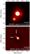 |
Fig. 1. SPHERE/IRDIS and NACO observations of the ET Cha system. The companion is well-resolved in the 2019 SPHERE epoch. We note that we show the primary star on a slightly saturated color scale in order to highlight the companion (the data is not saturated). In the 2003 NACO epoch the companion is close to the resolution limit of the instrument and shows as a strong asymmetrical extension to the primary star PSF. We have performed a high-pass filter to make the companion more clearly visible. We mark the companion position in the NACO image by two white bars. |
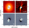 |
Fig. 2. Coronagraphic images of ET Cha taken with SPHERE/IRDIS in our program. Upper left: stacked total intensity image. Upper right: total intensity image after classical angular differential imaging reduction. Bottom: Stokes Q and U polarized flux images after polarization differential imaging. The size of the coronagraphic mask is indicated with the grey, hashed circle. The positive-negative signal pattern is caused by unresolved stellar polarization of the primary star, the companion or both and not by a resolved circumstellar disk. |
We performed polarimetric differential imaging on the coronagraphic data to search for polarized scattered light from the circumstellar disk around ET Cha. We show the final Stokes Q and U images in Fig. 2. We find a positive-negative signal pattern along the direction in which the stellar primary and companion are located. This is residual, unresolved stellar polarization and not resolved signal from a circumstellar disk. For a disk we would expect a “butterfly” pattern associated with azimuthal polarization (see e.g., Ginski et al. 2016). This is not present here. Stellar polarization is discussed in detail in van Holstein et al. (2020). The changing sign that we observe between the residual signal from the companion (in the south-east) and the stellar primary (in the north-west) suggests that both of these sources show different absolute linear polarization. Since both sources are co-located at the same distance, this cannot be introduced by different column densities of interstellar dust. Instead, it is likely that this is introduced by circumstellar material around the primary, the companion or both. We find the most likely explanation to be that the known circumstellar disk around the primary star is inclined and thus introduces a break in symmetry in the unresolved system. This would naturally result in a residual polarization of the light that we receive. However, since we do not know the exact geometry of the disk around the primary star, we can only speculate on the degree of linear polarization that is introduced. Thus, we cannot rule out that the light received from the companion is also intrinsically polarized, perhaps also by circumstellar material.
We conclude that we did not detect any significant signal from a resolved circumstellar disk outside of the inner working angle of the coronagraph. Due to the mis-centering, we conservatively estimate the inner working angle to be larger than the mask diameter, that is roughly 150 mas. We note that this inner working angle is asymmetric with closer separations sampled in the north-west than in the south-east.
In addition to the new SPHERE observations, we analyzed archival VLT/NACO data. In this data set, taken under excellent observing conditions, we find that the PSF of ET Cha is very clearly asymmetrically elongated towards the north-east (see Fig. 1, bottom panel). While such elongations are possible for other stars in the field-of-view due to the limited isoplanatic angle, they are not typical for the on-axis adaptive optics guide star itself. Furthermore, elongations due to isoplanatic angle effects are typically point-symmetric, while this is clearly not the case here. We thus conclude that in this NACO data set we recover the companion candidate detected by SPHERE. If this is the case, then the companion candidate has moved significantly relative to the primary star within the ∼17 year epoch difference between both data sets. In the following sections, we extract the astrometry and photometry of the companion from the data and discuss the nature of the object.
3.1. Astrometric analysis
Since the companion candidate was only well-detected in the SPHERE flux reference frames without a coronagraph, we used only these for astrometric extraction. The companion candidate is close to the primary star, which shows slightly asymmetric diffraction patterns, likely due to low-wind effect (ground wind speed was below 1 ms−1, see Cantalloube et al. 2019). It is thus difficult to remove either stellar PSF in absence of an independent reference PSF for the data set in order to measure individual stellar positions. We, therefore, fitted both the companion and the primary star position simultaneously. As model, we utilized two elliptical Moffat functions2. We allowed for ellipticity in the Moffat in order to better fit small asymmetries in the stellar PSFs of companion candidate and primary star. The initial guesses of the position were assigned by eye and then a least-squares fitting approach was utilized as implemented in the astropy model fitting package. The astrometric calibration for IRDIS was taken from Maire et al. (2016)3. The same fitting procedure was utilized for the NACO archival data. Since both data sets (SPHERE and NACO) were taken in the H-band, we fixed the flux ratio of the two fitted Moffat functions for the NACO data set to the flux ratio extracted from the SPHERE data (see Sect. 3.2). The astrometric calibration for NACO, taken from Chauvin et al. (2010), gives a pixel scale of 13.24 ± 0.05 mas pixel−1 with a true north correction of −0.05° ±0.10. The results are listed in Table 2 for both observing epochs.
Astrometry and photometry of the ET Cha system, as extracted from our SPHERE/IRDIS observations as well as NACO archival data.
We employed both astrometric epochs in order to check whether the companion candidate is co-moving with ET Cha on the sky. In Fig. 3, we show both data points relative to the expected behavior of a non-moving distant background star (grey, oscillating area in both panels). The existing astrometry is inconsistent with such an object. The dashed lines in Fig. 3 show the expected motion for a circular orbit. For the position angle, we considered a circular face-on orbit since it would lead to the maximum change of position angle, while for the separation, we considered an edge-on orbit since this would lead to the maximum change in separation over time. The companion candidate shows a change in position angle larger than expected for a circular face-on orbit (see Sect. 4.2 for a discussion of the system mass). However, we also see a significant increase in separation between the two observing epochs. This likely points to an orbit with an intermediate inclination or a non-zero eccentricity.
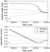 |
Fig. 3. SPHERE/IRDIS and NACO astrometry of the detected companion relative to the primary star versus time. Position angle is measured from north over east. The grey ribbon shows the expected location of a non-moving background object, while the dashed lines indicate possible circular orbital motion assuming a face-on orbit for position angle and an edge-on orbit for separation independently (these are mutual exclusive orbits to illustrate the maximum expected change in separation and position angle for the circular case). |
Given that the companion candidate is inconsistent with a distant background object, we estimated the probability to find a relatively nearby – that is, Galactic – background object within 0.15″ of ET Cha and with the limiting magnitude measured for the companion candidate. Such an object could, in theory, exhibit a non-zero proper motion and, thus, could mimic a co-moving bound companion. For this, we used the approach by Lillo-Box et al. (2014) and the TRILEGAL v1.6 population synthesis models (Girardi et al. 2012). We find the probability is 10−6, that is, negligible. Thus, we conclude from the astrometric and probability analysis that the detected source is in all likelihood a true bound companion to the ET Cha system.
3.2. Photometric analysis
We used the SPHERE/IRDIS flux calibration frames to extract relative photometry between the primary star and the companion. Since we do not have a reference PSF that is not contaminated by the close companion, we applied aperture photometry. Aperture radii of three pixels (36.8 mas) were used for both objects. To achieve an accurate measurement, we estimated the cross-contamination of the companion and the primary PSF in several ways. We subtracted an azimuthally averaged profile of the primary PSF as well as a 180° rotated profile. We also measured the unaltered companion flux and subtracted the average background flux at the same separation but opposite side of the primary star. Between these measurements, we find an ∼8% variation in the recovered flux. We ultimately adopted the average value of these measurements for the companion and considered the variation in flux as uncertainty. Additionally, we included the standard deviation of the background in the uncertainty of the photometric result listed in Table 2. Since the companion is at the resolution limit in the NACO observation and was observed in the same band as the IRDIS observation, we did not attempt to extract photometry from the NACO data set.
To calculate the apparent magnitude of the companion we used the H-band measurement of the system listed in the 2MASS catalog (Cutri et al. 2003) of 9.834 ± 0.021 mag. This measurement does not resolve the primary star and the companion and, thus, it represents the combined flux. To correct for the contribution of the companion, we use the formula presented in Bohn et al. (2020). We find a correction of 0.23 mag. Thus, we compute an apparent magnitude for the companion of 11.65 ± 0.07 mag.
4. The age and mass of ET Cha
In order to determine the mass of the newly detected companion from photometry, we need to know its age. In the following, we first discuss the ET Cha system age, based on cluster age, kinematics, and stellar parameters of the primary star. We then use this age estimate together with (sub)stellar isochrone models to determine the companion mass.
4.1. Age estimate of the system
The age of the η Cha cluster has been the subject of intense study. In the initial study by Mamajek et al. (1999), a large spread of individual system ages was found ranging from 2 Myr to 18 Myr from compiled photometry, leading to an average age of ∼8 Myr (Mamajek et al. 2000). The study by Lawson et al. (2001) is broadly in agreement, inferring an age range between 4 Myr and 9 Myr for the M-star members of the cluster from re-compiled H-R-diagrams. An isochronal analysis of the color-magnitude data for the cluster members by Bell et al. (2015) yielded an older cluster age of 11 ± 3 Myr on an age scale consistent with results from Li depletion boundary analyses of other well-studied young clusters (e.g., Soderblom et al. 2014). However, we note that Herczeg & Hillenbrand (2015) find a significantly younger average age of 5.5 ± 1.3 Myr (but with a spread between 2.1 Myr and 12.7 Myr) from a comparison of the available literature photometry and spectral types of cluster members with various stellar model isochrones.
The best age estimate for a cluster member is available for the RS Cha system (RECX 8). A comparison of the stellar parameters for this well-constrained intermediate-mass (A8V + A8V) eclipsing binary to modern evolutionary tracks have yielded ages of 9.1 ± 2 Myr (Alecian et al. 2007) and 8.0 Myr (Gennaro et al. 2012).
Due to the seemingly large age spread within the cluster, it is problematic to assign the cluster age to individual sources. ET Cha is one of only two known members of η Cha with a gas-rich class II disk, giving some indication that the system might in fact be younger than the average cluster age. Woitke et al. (2011) note that the near-infrared colors seen in ET Cha are a better fit to a disk that is 1−2 Myr old. We discuss two scenarios to estimate the age of the ET Cha system.
ET Cha age estimate from stellar parameters. Recently Rugel et al. (2018) published medium spectral resolution X-Shooter spectra of ET Cha taken simultaneously in the optical and near infrared. From these spectra, they calculate the stellar properties and find an effective temperature of 3190 K, as well as a stellar luminosity of 0.073 L⊙. We used these values as input for Siess et al. (2000) evolutionary models as well as Baraffe et al. (2015) models. We find an age of 4.9 Myr for the former and an even younger age of 3.2 Myr for the latter model. These age estimates are on the lower end of the range for M-star cluster member proposed by Lawson et al. (2001). To remain consistent with all age estimates, we thus favor the age of 4.9 Myr obtained from the Siess model tracks.
ET Cha age estimate from kinematics. Isochronal model tracks are known to underestimate the age of low-mass stars (Pecaut et al. 2012; Bell et al. 2015; Pecaut & Mamajek 2016). Thus, ET Cha could be older than estimated from its stellar parameters using such models. There is, in fact, some compelling kinematic evidence that the system may be part of the well-characterized RS Cha system. RS Cha is located only 68″ to the north-west of ET Cha. RS Cha shows a proper motion of −27.168 ± 0.072 mas yr−1 in RA and 28.015 ± 0.073 mas yr−1 in Dec as measured by Gaia DR2. ET Cha has a proper motion of −27.343 ± 0.487 mas yr−1 in RA and 27.323 ± 0.571 mas yr−1 in Dec, which means that the motion in RA is within 1σ of RS Cha and the motion in Dec is within 2σ of RS Cha. Converting the differences in their proper motions vectors to tangential velocity (assuming d = 100 pc for simplicity), their tangential motions agree within 0.34 ± 0.36 km s−1. Using inverse Gaia parallaxes the systems are at face value located at different distances, that is, RS Cha at 99.0 ± 0.4 pc and ET Cha at 91.7 ± 2.5 pc. However, our findings show that ET Cha is a close binary star with a separation of 135 mas. Assuming a simple circular orbit for the pair, we find that during the Gaia DR2 period, the orbital displacement of ET Cha may have been of the order of 1 mas4. This additional uncertainty allows for the possibility that ET Cha is located at slightly larger and possibly the same distance as RS Cha. If this is the case, then it is highly unlikely that the system is younger than RS Cha. We conclude that it currently cannot be ruled out that ET Cha and RS Cha are forming a wide multiple system. In this case, ET Cha should be co-eval with RS Cha and we adopt an age of 8 Myr for this scenario.
4.2. Mass estimates for primary and secondary
Given the age estimate and the photometry, we can estimate the masses of the primary star and the companion in the ET Cha system. To compute absolute magnitudes from our photometric analysis, we have to assume a distance of the system. In the case that ET Cha is not associated with RS Cha and, thus, 5 Myr old, we use the Gaia DR2 parallax measurement of 91.7 pc. However, if we assume that ET Cha and RS Cha form a wide pair, then they should be located at roughly the same distance and the Gaia parallax measurement for ET Cha is likely flawed. For this scenario we thus adopt the distance measurement of RS Cha, that is, 99.0 pc.
Using BT-SETTL model isochrones for low-mass stars and brown dwarfs (Baraffe et al. 2015), we find masses of 0.22 M⊙ and 0.048 M⊙ (50.3 MJup) for the primary star and companion, respectively for the first scenario. Using the older age and larger distance, we find values of 0.32 M⊙ and 0.10 M⊙.
5. Limits on additional companions
Using the deep coronagraphic total intensity images, we investigated the possible presence of further companions to the ET Cha system. For this purpose, we applied the TLOCI angular differential imaging algorithm (Marois et al. 2014) as realized in the SpeCal toolbox (Galicher et al. 2018) implemented into the SPHERE-DC reduction pipeline (Delorme et al. 2017). We find two additional point sources at separations of 3.03 ± 0.02 arcsec and 4.20 ± 0.02 arcsec, along with position angles of 82.1° ± 0.3° and 135.2° ± 0.3°. The closer of these is also detected in the NACO archival data and is consistent with a distant, non-moving background object (see Fig. A.1). The farther source is too faint (21.3 ± 0.2 mag in the SPHERE H-band image) to be detected in the NACO data. Thus, we cannot determine its nature. However, due to its wide separation, it seems likely that this is a background source as well.
Using the procedure outlined in Galicher et al. (2018), we use the total intensity data to determine detection limits for additional companions. The result is shown in Fig. 4. Utilizing models by Baraffe et al. (2015), we can translate the contrast limits to mass limits. We can rule out additional stellar or brown dwarf companions down to an angular separation of ∼190 mas independent of the system age. Outside of 1″ we are sensitive to planetary mass companions down to masses of 3 MJup for the lower system age and down to 4 MJup for the higher system age.
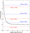 |
Fig. 4. Contrast limits derived from the coronagraphic observations using angular differential imaging and TLOCI post-processing. Mass limits for the 5 Myr and the 8 Myr case are indicated with the blue, dash-dotted lines and the red, dashed lines, respectively. |
6. Orbit analysis of the ET Cha system
We utilized the orbitize! Python package (Blunt et al. 2020) to investigate possible orbit configurations of the system. We employed the OFTI (Blunt et al. 2017) sampling method with 106 runs. We consider the two scenarios for the system mass discussed in the previous section, that is, a total mass of 0.268 M⊙ for the younger low-mass scenario 1 and a total mass of 0.42 M⊙ for the older higher-mass scenario 2. In addition use different distance estimates for scenario 1 and scenario 2, that is, 91.7 pc and 99.0 pc, respectively. Since we only have two astrometric data points and the primary goal is to get a general understanding of possible orbit families, we do not consider an uncertainty for the mass estimates in the fit, meaning that they are treated as fixed values and not free parameters. The resulting posterior distributions of semi-major axis, inclination, and eccentricity are shown in Fig. 5. We additionally show ten randomly selected orbits for both mass scenarios in Appendix B. We note that while we do not limit the semi-major axis to a certain parameter range, we cut off the posterior distributions shown here at 30 au. This is motivated by Bate (2009), who find in their hydrodynamic simulations of stellar clusters that low-mass binaries typically have a semi-major axis smaller than 30 au. We cannnot, however, at this time put a meaningful upper limit on the semi-major axis. Extreme eccentric solutions with very large semi-major axis up to ∼1000 au are, in principle, consistent with the astrometric data points.
 |
Fig. 5. Resulting orbit solutions for the ET Cha system using our extracted astrometry. We utilized the orbitize! package and the included OFTI algorithm with 106 generated orbits. We show semi-major axis, inclination, and eccentricity. Scenario 1 is in the lower left corner in blue color and scenario 2 is in the upper right corner in red. |
While we can not constrain the orbit tightly from only two data points, we find that several bound orbit families exist. We find typically either inclined or eccentric orbits or a mixture of both, and we can rule out circular face-on orbits. The degeneracy between inclination and eccentricity is typical for an orbit with a low coverage of data points or with only short orbital arcs observed (see e.g., Ginski et al. 2014).
Low-mass scenario 1. For the low-mass scenario 1, we find a first-orbit family with the most likely inclination range between 30° and 73°, that is, the inclination is rather unconstrained. These solutions can be circular, but have the strongest probability peak between eccentricities of 0.15 and 0.3. The most likely semi-major axis range is 9 au to 15 au with a peak at 13 au. A second orbit family favors high eccentricity values of roughly 0.2 to 0.75 which correspond to slightly smaller semi-major axes between 8 au and 11 au with peak at 8.5 au. These solutions have a smaller inclination roughly between 0° and 40°. We find a general lower limit of the semi-major axis across all solutions of 6.5 au but can neither constrain inclination nor eccentricity to any upper or lower values.
High-mass scenario 2. For the higher mass scenario 2, we find, similarly, two-orbit families. The high-inclination family shows a probability peak in the inclination between 55° and 75°. These solutions have, most likely, a semi-major axis range between 10 au and 19 au, with a strong peak at 14 au. These solutions can be circular and have the strongest probability between eccentricities of 0 and 0.2. Compared to the lower mass scenario, we thus find that for this first orbit family high inclinations, larger semi-major axis, but lower eccentricities are preferred. The second orbit family contains the more eccentric solutions with a probability peak in the eccentricity space between 0.4 and 0.7. These solutions have smaller semi-major axes with a peak between 9 au and 10 au. As was the case for the lower mass scenario, these solutions have smaller inclinations, which are roughly between 0° and 40°. Thus, this second-orbit family is located in a very similar parameter space to the lower mass scenario.
While this first assessment of the system orbit is instructive, we caution that this picture might change significantly with the addition of even one well-calibrated observing epoch.
7. Discussion
Our photometric and age analysis finds that the companion is either a low-mass (0.10 M⊙) pre-main-sequence M-type star or a brown dwarf (0.048 M⊙, i.e., 50.3 MJup), depending on the system age. Accordingly, the mass ratio between primary star and companion is either 0.31 or 0.21 (with the primary star itself also having an age-dependent mass). In both cases, this makes for a somewhat atypical system. Bate (2009) found with hydrodynamic simulations of stellar clusters that the median mass ratio for binary systems with a semi-major axis smaller than 10 au is 0.74 and for systems with semi-major axis between 10 au and 100 au is 0.57. This theoretical result is supported also by observational surveys, for example, Delfosse et al. (2004) find that brown dwarf companions are rare within 100 au from main-sequence M-dwarf primary stars (∼1% of their sample stars had a brown dwarf companion). For more, see Duchêne & Kraus (2013) and references therein, where similar results are discussed for pre-main-sequence stars. On the other hand, Bate (2009) also finds that the separation between binary components depends strongly on the primary mass, that is, it increases with increasing mass. For primary masses between 0.2 M⊙ and 0.5 M⊙, they find a bi-modal distribution with roughly half of the recovered systems exhibiting semi-major axis smaller than 10 au, that is, compatible with a large fraction of the recovered orbit solutions for ET Cha.
7.1. The formation of the ET Cha system
There are several possible formation pathways for systems like ET Cha. The most prominent ones are either fragmentation in the proto-stellar cloud (e.g., Bate et al. 1995; Kroupa 1995; Lomax et al. 2015; Moe et al. 2019) and gravitational instability in the proto-stellar or circumstellar disk (e.g., Boss 1997; Kratter & Lodato 2016). Both of these mechanisms will (at least initially) produce dynamically very different systems. While an object formed via cloud fragmentation can show strong spin-orbit misalignment and potential high orbit eccentricities, this would not be expected from an object formed in a disk around the primary star. Both mass scenarios for the ET Cha system produce an appreciable number of eccentric orbit solutions. These are in particular preferred for the lower mass scenario in which the system is younger and the new detected companion in the brown dwarf regime.
However, objects formed via fragmentation in a disk may also exhibit eccentric orbits if they experienced dynamic encounters. Reipurth & Clarke (2001) suggest scattering of low-mass cores in multiple systems as a main formation pathway to explain wide orbit brown dwarfs. For this, a third body would be needed, which is so far not observed in the ET Cha system. Such a body could either be in a close orbit around ET Cha, it could have fallen into ET Cha A or it could potentially be another cluster member. The possibility that ET Cha is bound to RS Cha would make this a complex multiple system. A dynamical scattering of the ET Cha system by another cluster member may also be supported by findings of Moraux et al. (2007). They simulated the η Cha cluster and found that ejection of cluster members may have occurred with most objects ejected in the early stages of formation, after roughly 1−4 Myr. In their simulation, they find ejection velocities of 1−5 km s−1, which translates into a distance of 9 pc from the cluster core after 7 Myr. Such ejected members of the η Cha cluster were indeed found by Murphy et al. (2010). They suggest a halo of low-mass members of the cluster within 5 5 from the cluster center, that is, within 9 pc. In this scenario, ET Cha would be a member of this low-mass halo which was ejected towards us. If the Gaia parallax is taken at face value it may support such a history of ET Cha since it is located roughly 7 pc closer than the median of the η Cha cluster (see Fig. C.1). However, we caution that such a scenario in which the system is ejected directly toward us seems unlikely.
Besides the dynamical signatures, there are several numerical studies that give some evidence to the formation history of the system. Most notably, Vorobyov (2013) performed simulations of disk gravitational fragmentation and found that they were unable to produce brown dwarf companions at small orbital separations. Furthermore, Kratter et al. (2010), Offner et al. (2010), and Haworth et al. (2020) found that disk fragmentation is less likely around M-dwarf primary stars. We suggest, thus, that some circumstantial evidence exists to support the formation of ET Cha B via core fragmentation in the proto-stellar cloud.
7.2. Interaction with the circumstellar disk
The circumstellar disk around the primary star was not detected in our scattered light observations down to an average5 separation of 0.0925″ (8.5−9.2 au, depending on the system distance), that is, the nominal inner working angle of the employed coronagraph. This confirms its previously inferred small radius (5−7 au, see Woitke et al. 2019). The ALMA surveys of recent years have shown that such small disks are not uncommon (see e.g. Ansdell et al. 2016). Given the newly detected close B component, the small size of the disk is indeed not surprising and is likely explained by truncation. In such a case, the expected disk outer radius is half the periastron separation (Hall et al. 1996). The closest projected separation was observed with NACO to be 50.5 mas. If we assume that this is the actual physical separation at periastron, then the disk should have been truncated at 2.3−2.5 au. However, this assumes that the entire orbital trajectory is in the plane of the sky, which might well not be the case (we recover many orbits with larger periastron separations). So this should be seen as a lower limit and is, in principle, consistent with the inferred disk radius of 5−7 au. Truncation by outer companions is indeed common. Manara et al. (2019) recently found that disks in known multiple systems are systematically smaller in mm continuum emission than their counter parts around single stars.
The disk around ET Cha is still unusual in several aspects. Kraus et al. (2012) find from an observational study in Taurus that the disk frequency is significantly reduced around close (≤50 au) binaries. While they find disks in more than ∼80% of wide binaries (same result as for single stars), this is true for only ∼40% of close binaries. These results are supported by recent population synthesis models by Rosotti & Clarke (2018), who find that binaries with separations similar to ET Cha (∼10 au) only have a disk in 10% of the cases. In the same study, they predict that in these close systems, the disk around the secondary component will clear first, which is in line with our non-detection of a resolved disk around the B component.
A second puzzling aspect of the system is its high accretion rate. Using the UV excess measurement Rugel et al. (2018) estimated an accretion rate of 7.6 × 10⁻¹⁰ M⊙ yr−1. Assuming a gas mass of 1.2 × 10⁻⁴ M⊙ (Woitke et al. 2019) and a constant accretion rate, the circumstellar disk should be gone after only ∼1.6 × 10⁵ yr−1, that is, a time frame that is much shorter than both our estimates for the system age. However Rosotti & Clarke (2018) found that a close companion has significant influence on the evolution of the disk. In particular, for a semi-major axis smaller than 20−30 au, the dominating disk dispersal mechanism changes from the inside-out regime (through photo-evaporation) to the outside-in regime due to the tidal torque of the companion. Thus, in these disks, no inner cavity is opened, which leads to significantly higher accretion rates than those for wide separation binary stars or single stars. In particular, the dimensionless η parameter that was studied by Jones et al. (2012) and Rosotti et al. (2017) which is the product of system age and accretion time divided by disk mass, shows a steep increase with age for these systems. For ET Cha, we compute values for η of 31 and 51 for the younger and older disk age. Such values are possible in the simulations by Rosotti et al. (2017), but given the system separation, they imply an age younger than 1.5 Myr for a value of the viscous parameter α (Shakura & Sunyaev 1976) of 10−3.
To reconcile the age and accretion rate of ET Cha, we require a lower viscous parameter α of 10−4. This would increase the disk viscous timescale at a truncation radius of 10 au to 5 Myr. Since the disk dispersal takes on the order of 2−3 viscous timescales (Pringle 1981; Rosotti & Clarke 2018) the presence of the disk in both age scenarios would then not be problematic. However, lowering the viscous timescale would also imply that we need a higher disk mass to explain the current high accretion rate (assuming purely viscous accretion). We roughly find that an increase by a factor 10−15 would be required. The disk mass could be indeed significantly higher than that inferred by Woitke et al. (2019) if the disk is optically thick outside of 1 au.
We note that very recently Manara et al. (2020) found similarly high accretion rates reported for ET Cha around several members of the ∼5 Myr Upper Scorpius region (see also Ingleby et al. 2014; Venuti et al. 2019 for Orion OB1 and TWA). The mass estimate in this case was based on the dust. They suggest that a higher gas-to-dust ratio than the often assumed 100 would explain the measured accretion rates. Indeed Woitke et al. (2019) find with their thermo-chemical modeling of the ET Cha system an extreme gas-to-dust ratio of 3500 and the true value would be even more extreme if the gas mass is indeed underestimated. However, it would be very interesting to study the sample of Manara et al. (2020) with high angular resolution to test the correlation of a high accretion rate with the occurrence rate of close companions.
We find that another scenario might simultaneously explain the discrepancy of the age and accretion rate of the system, as well as the small size of the circumstellar disk. If the companion is not bound but, instead, is on a hyperbolic orbit, that is, we image the system close to the periastron passage during a fly-by, then the disk could have been recently truncated. However, we do not see evidence for a dispersing disk outside of the companion orbit. Also, such a scenario is inherently unlikely because close encounters are rare (Adams et al. 2006; Winter et al. 2018) and it is even more unlikely to observe them close to periastron passage. We nevertheless include for completeness that with only two astrometric epochs, we cannot rule out a hyperbolic orbit (even though we did not specifically fit unbound trajectories). Finally, it may be possible that the accretion rate is highly variable if accretion “pulses” are triggered by the companion during periastron passage of an eccentric orbital trajectory (e.g., Tofflemire et al. 2019).
8. Summary and conclusion
We detected a low-mass (50.3 MJup or 0.1 M⊙, depending on system age) companion to the η Cha cluster member ET Cha. This companion is inconsistent with a background object and, in all likelihood, it is associated with ET Cha. From SPHERE and NACO measurements spaced almost 17 years apart, we can see significant orbital motion, which can be explained by several families of bound orbits, many of them with significant eccentricity. Due to a lack of additional data points, we cannot rule out hyperbolic orbits.
The mass ratio of the system is low compared to theoretical and observational studies, possibly representing an extreme case of a young multi-star system. From the small separation, low-mass ratio, and potential eccentric orbit, we tentatively conclude that the companion may have formed via fragmentation in the proto-stellar cloud.
The disk around ET Cha has several particular characteristics, such as its small outer radius, its high gas-to-dust ratio, and high accretion rate as compared to age and gas mass, which may all be well-explained by the companion. In particular, the small separation of the pair indicates that the disk clearing might be dominated by tidal torques from the companion, which also trigger the high accretion rate. If we assume purely viscous accretion, then we find that we need a low α of ∼10−4 to explain the presence of the disk at the age of the system. This is in line with with recent studies of multi-ringed disks, which also require a low viscosity (Dullemond et al. 2018). To come to more definitive conclusions regarding the evolutionary state of the system and its dynamical history, follow-up observations are required. In particular, we suggest the following:
-
SPHERE/IRDIS follow-up observations spread over the next few years to determine the orbit of the system, particularly if the orbit is bound and if it is highly eccentric.
-
A search for accretion tracers of the companion, which may indicate in-situ formation or very recent ejection from the inner system. This may be done with SPHERE/ZIMPOL or VLT/MUSE in Hα or possibly MagAO-X once it is online.
-
Non-coronagraphic follow-up observations with SPHERE/IRDIS to determine the polarization state of both objects and thus infer (or rule out) the presence of circumstellar material around the companion.
-
VLT/ERIS measurements (once the instrument is available) to get a companion spectrum and possibly its radial velocity, which would significantly constrain its orbit as well as mass.
-
Very high spatial resolution (about 3 au should be possible) and sensitive ALMA observations of the gas and dust. Such observations can provide stringent constraints on the gas and dust mass, the extension of the disk, and the presence of a (remnant) circumbinary disk. Furthermore, the spectral line observations, with the necessary spectral resolution, can provide additional constrains on the mass of the primary.
Stellar multiplicity can generally have a strong influence on the evolution of circumstellar disks. Our new observations show that with extreme adaptive-optics instruments, it is now possible to detect previously unnoticed (sub)stellar companions to young stars, particularly in a parameter range (separation and mass) where they may cause significant changes in disk evolution. Currently, instruments such as SPHERE and GPI, are limited in their target sample by the requirements of optically bright guide stars for their adaptive optics systems. This leads to an observational bias towards the higher end of the mass function. This is one of the many reasons why instrument upgrades such as the proposed SPHERE+ concept (Boccaletti et al. 2020) are highly important for furthering the understanding of the evolution of young systems.
We note that, while still rare, there is an increasing number of “old” systems with signs of ongoing accretion discovered in the recent literature. See Lee et al. (2020) for an example.
In an upcoming publication (Ginski et al., in prep.), we extensively tested the influence of different fitted model functions on the retrieved astrometry for tight binary stars with SPHERE/ZIMPOL. We found that as long as the model has a well defined peak the astrometric result was virtually identical.
We note that the calibration was performed in standard imaging mode and not DPI mode. In DPI mode an extra half-wave-plate is inserted into the beam path. We have at this time no evidence that this alters the astrometric solution.
While the same uncertainty could affect the proper motion, here longer baselines are available, which limit the influence of this deviation.
As noted previously the mask was misaligned, thus, we probe closer to the star in the north-west and slightly further away from the star in the south-east.
Acknowledgments
The authors would like to thank Anthony Brown for fruitful discussions. SPHERE is an instrument designed and built by a consortium consisting of IPAG (Grenoble, France), MPIA (Heidelberg, Germany), LAM (Marseille, France), LESIA (Paris, France), Laboratoire Lagrange (Nice, France), INAF – Osservatorio di Padova (Italy), Observatoire de Genève (Switzerland), ETH Zurich (Switzerland), NOVA (Netherlands), ONERA (France), and ASTRON (The Netherlands) in collaboration with ESO. SPHERE was funded by ESO, with additional contributions from CNRS (France), MPIA (Germany), INAF (Italy), FINES (Switzerland), and NOVA (The Netherlands). SPHERE also received funding from the European Commission Sixth and Seventh Framework Programmes as part of the Optical Infrared Coordination Network for Astronomy (OPTICON) under grant number RII3-Ct2004-001566 for FP6 (2004-2008), grant number 226604 for FP7 (2009-2012), and grant number 312430 for FP7 (2013-2016). C. G. acknowledges funding from the Netherlands Organisation for Scientific Research (NWO) TOP-1 grant as part of the research program “Herbig Ae/Be stars, Rosetta stones for understanding the formation of planetary systems”, project number 614.001.552. EEM acknowledges support from NASA award 17-K2GO6-0030. Part of this research was carried out at the Jet Propulsion Laboratory, California Institute of Technology, under a contract with the National Aeronautics and Space Administration (NASA). FMe acknowledges funding from ANR of France under contract number ANR-16-CE31-0013. GR acknowledges funding from the Dutch Research Council (NWO) with project number 016.Veni.192.233. R. A.-T. acknowledges support from the European Research Council under the Horizon 2020 Framework Program via the ERC Advanced Grant Origins 83 24 28. T. B. acknowledges funding from the European Research Council under the European Union’s Horizon 2020 research and innovation programme under grant agreement No 714769 and funding from the Deutsche Forschungsgemeinschaft under Ref. no. FOR 2634/1 and under Germanys Excellence Strategy (EXC-2094–390783311). This work has made use of the SPHERE Data Centre, jointly operated by OSUG/IPAG (Grenoble), PYTHEAS/LAM/CESAM (Marseille), OCA/Lagrange (Nice), Observatoire de Paris/LESIA (Paris), and Observatoire de Lyon. This research has used the SIMBAD database, operated at CDS, Strasbourg, France (Wenger et al. 2000). We used the Python programming language (Python Software Foundation, https://www.python.org/), especially the SciPy (Virtanen et al. 2020), NumPy (Oliphant 2006), Matplotlib (Hunter 2007), photutils (Bradley et al. 2016), and astropy (Astropy Collaboration 2013, 2018) packages. We thank the writers of these software packages for making their work available to the astronomical community.
References
- Adams, F. C., Proszkow, E. M., Fatuzzo, M., & Myers, P. C. 2006, ApJ, 641, 504 [NASA ADS] [CrossRef] [Google Scholar]
- Alecian, E., Goupil, M. J., Lebreton, Y., Dupret, M. A., & Catala, C. 2007, A&A, 465, 241 [NASA ADS] [CrossRef] [EDP Sciences] [Google Scholar]
- Andrews, S. M., Rosenfeld, K. A., Kraus, A. L., & Wilner, D. J. 2013, ApJ, 771, 129 [NASA ADS] [CrossRef] [Google Scholar]
- Andrews, S. M., Huang, J., Pérez, L. M., et al. 2018, ApJ, 869, L41 [NASA ADS] [CrossRef] [Google Scholar]
- Ansdell, M., Williams, J. P., van der Marel, N., et al. 2016, ApJ, 828, 46 [Google Scholar]
- Astropy Collaboration (Robitaille, T. P., et al.) 2013, A&A, 558, A33 [NASA ADS] [CrossRef] [EDP Sciences] [Google Scholar]
- Astropy Collaboration (Price-Whelan, A. M., et al.) 2018, AJ, 156, 123 [Google Scholar]
- Baraffe, I., Homeier, D., Allard, F., & Chabrier, G. 2015, A&A, 577, A42 [NASA ADS] [CrossRef] [EDP Sciences] [Google Scholar]
- Bate, M. R. 2009, MNRAS, 392, 590 [NASA ADS] [CrossRef] [Google Scholar]
- Bate, M. R., Bonnell, I. A., & Price, N. M. 1995, MNRAS, 277, 362 [NASA ADS] [CrossRef] [Google Scholar]
- Bell, C. P. M., Mamajek, E. E., & Naylor, T. 2015, MNRAS, 454, 593 [NASA ADS] [CrossRef] [Google Scholar]
- Beuzit, J. L., Vigan, A., Mouillet, D., et al. 2019, A&A, 631, A155 [NASA ADS] [CrossRef] [EDP Sciences] [Google Scholar]
- Blunt, S., Nielsen, E. L., De Rosa, R. J., et al. 2017, AJ, 153, 229 [NASA ADS] [CrossRef] [Google Scholar]
- Blunt, S., Wang, J. J., Angelo, I., et al. 2020, AJ, 159, 89 [CrossRef] [Google Scholar]
- Boccaletti, A., Chauvin, G., Mouillet, D., et al. 2020, ArXiv e-prints [arXiv:2003.05714] [Google Scholar]
- Bohn, A. J., Southworth, J., Ginski, C., et al. 2020, A&A, 635, A73 [NASA ADS] [CrossRef] [EDP Sciences] [Google Scholar]
- Boss, A. P. 1997, Science, 276, 1836 [NASA ADS] [CrossRef] [Google Scholar]
- Bradley, L., Sipocz, B., Robitaille, T., et al. 2016, Astrophysics Source Code Library [record ascl:1609.011] [Google Scholar]
- Cantalloube, F., Dohlen, K., Milli, J., Brandner, W., & Vigan, A. 2019, The Messenger, 176, 25 [NASA ADS] [Google Scholar]
- Carbillet, M., Bendjoya, P., Abe, L., et al. 2011, Exp. Astron., 30, 39 [NASA ADS] [CrossRef] [Google Scholar]
- Chauvin, G., Lagrange, A. M., Bonavita, M., et al. 2010, A&A, 509, A52 [NASA ADS] [CrossRef] [EDP Sciences] [Google Scholar]
- Cutri, R. M., Skrutskie, M. F., van Dyk, S., et al. 2003, VizieR Online Data Catalog: II/246 [Google Scholar]
- de Boer, J., Langlois, M., van Holstein, R. G., et al. 2020, A&A, 633, A63 [NASA ADS] [CrossRef] [EDP Sciences] [Google Scholar]
- Delfosse, X., Beuzit, J. L., Marchal, L., et al. 2004, in M Dwarfs Binaries: Results from Accurate Radial Velocities and High Angular Resolution Observations, eds. R. W. Hilditch, H. Hensberge, & K. Pavlovski, ASP Conf. Ser., 318, 166 [Google Scholar]
- Delorme, P., Meunier, N., Albert, D., et al. 2017, in SF2A-2017: Proceedings of the Annual Meeting of the French Society of Astronomy and Astrophysics, eds. C. Reylé, P. Di Matteo, F. Herpin, et al., 347 [Google Scholar]
- Devillard, N. 1999, in Infrared Jitter Imaging Data Reduction: Algorithms and Implementation, eds. D. M. Mehringer, R. L. Plante, & D. A. Roberts, ASP Conf. Ser., 172, 333 [Google Scholar]
- Duchêne, G., & Kraus, A. 2013, ARA&A, 51, 269 [Google Scholar]
- Dullemond, C. P., Birnstiel, T., Huang, J., et al. 2018, ApJ, 869, L46 [NASA ADS] [CrossRef] [EDP Sciences] [Google Scholar]
- Fedele, D., van den Ancker, M. E., Henning, T., Jayawardhana, R., & Oliveira, J. M. 2010, A&A, 510, A72 [NASA ADS] [CrossRef] [EDP Sciences] [Google Scholar]
- Galicher, R., Boccaletti, A., Mesa, D., et al. 2018, A&A, 615, A92 [NASA ADS] [CrossRef] [EDP Sciences] [Google Scholar]
- Garufi, A., Benisty, M., Pinilla, P., et al. 2018, A&A, 620, A94 [NASA ADS] [CrossRef] [EDP Sciences] [Google Scholar]
- Gennaro, M., Prada Moroni, P. G., & Tognelli, E. 2012, MNRAS, 420, 986 [NASA ADS] [CrossRef] [Google Scholar]
- Ginski, C., Schmidt, T. O. B., Mugrauer, M., et al. 2014, MNRAS, 444, 2280 [NASA ADS] [CrossRef] [Google Scholar]
- Ginski, C., Stolker, T., Pinilla, P., et al. 2016, A&A, 595, A112 [NASA ADS] [CrossRef] [EDP Sciences] [Google Scholar]
- Girardi, L., Barbieri, M., Groenewegen, M. A. T., et al. 2012, Astrophys. Space Sci. Proc., 26, 165 [Google Scholar]
- Greaves, J. S., & Rice, W. K. M. 2010, MNRAS, 407, 1981 [NASA ADS] [CrossRef] [Google Scholar]
- Haisch, K. E., Jr., Lada, E. A., & Lada, C. J. 2001, ApJ, 553, L153 [NASA ADS] [CrossRef] [Google Scholar]
- Hall, S. M., Clarke, C. J., & Pringle, J. E. 1996, MNRAS, 278, 303 [NASA ADS] [Google Scholar]
- Haworth, T. J., Cadman, J., Meru, F., et al. 2020, MNRAS, 494, 4130 [CrossRef] [Google Scholar]
- Herczeg, G. J., & Hillenbrand, L. A. 2015, ApJ, 808, 23 [Google Scholar]
- Hernández, J., Calvet, N., Briceño, C., et al. 2007, ApJ, 671, 1784 [NASA ADS] [CrossRef] [Google Scholar]
- Hunter, J. D. 2007, Comput. Sci. Eng., 9, 90 [NASA ADS] [CrossRef] [Google Scholar]
- Ingleby, L., Calvet, N., Hernández, J., et al. 2014, ApJ, 790, 47 [NASA ADS] [CrossRef] [Google Scholar]
- Jones, M. G., Pringle, J. E., & Alexander, R. D. 2012, MNRAS, 419, 925 [NASA ADS] [CrossRef] [Google Scholar]
- Kratter, K., & Lodato, G. 2016, ARA&A, 54, 271 [NASA ADS] [CrossRef] [Google Scholar]
- Kratter, K. M., Matzner, C. D., Krumholz, M. R., & Klein, R. I. 2010, ApJ, 708, 1585 [NASA ADS] [CrossRef] [Google Scholar]
- Kraus, A. L., Ireland, M. J., Hillenbrand, L. A., & Martinache, F. 2012, ApJ, 745, 19 [NASA ADS] [CrossRef] [Google Scholar]
- Kroupa, P. 1995, MNRAS, 277, 1491 [NASA ADS] [CrossRef] [Google Scholar]
- Langlois, M., Dohlen, K., Vigan, A., et al. 2014, in High Contrast Polarimetry in the Infrared with SPHERE on the VLT, SPIE Conf. Ser., 9147, 91471R [Google Scholar]
- Lawson, W. A., Crause, L. A., Mamajek, E. E., & Feigelson, E. D. 2001, MNRAS, 321, 57 [NASA ADS] [CrossRef] [Google Scholar]
- Lawson, W. A., Crause, L. A., Mamajek, E. E., & Feigelson, E. D. 2002, MNRAS, 329, L29 [NASA ADS] [CrossRef] [MathSciNet] [Google Scholar]
- Lawson, W. A., Lyo, A. R., & Muzerolle, J. 2004, MNRAS, 351, L39 [NASA ADS] [CrossRef] [Google Scholar]
- Lee, J., Song, I., & Murphy, S. 2020, MNRAS, 494, 62 [CrossRef] [Google Scholar]
- Lenzen, R., Hartung, M., Brandner, W., et al. 2003, in NAOS-CONICA First on Sky Results in a Variety of Observing Modes, eds. M. Iye, & A. F. M. Moorwood, SPIE Conf. Ser., 4841, 944 [Google Scholar]
- Lillo-Box, J., Barrado, D., & Bouy, H. 2014, A&A, 566, A103 [NASA ADS] [CrossRef] [EDP Sciences] [Google Scholar]
- Lomax, O., Whitworth, A. P., Hubber, D. A., Stamatellos, D., & Walch, S. 2015, MNRAS, 447, 1550 [NASA ADS] [CrossRef] [Google Scholar]
- Lyo, A. R., Lawson, W. A., Mamajek, E. E., et al. 2003, MNRAS, 338, 616 [NASA ADS] [CrossRef] [Google Scholar]
- Maire, A. L., Langlois, M., Dohlen, K., et al. 2016, in SPHERE IRDIS and IFS Astrometric Strategy and Calibration, SPIE Conf. Ser., 9908, 990834 [Google Scholar]
- Mamajek, E. E., Lawson, W. A., & Feigelson, E. D. 1999, ApJ, 516, L77 [NASA ADS] [CrossRef] [Google Scholar]
- Mamajek, E. E., Lawson, W. A., & Feigelson, E. D. 2000, ApJ, 544, 356 [NASA ADS] [CrossRef] [Google Scholar]
- Manara, C. F., Morbidelli, A., & Guillot, T. 2018, A&A, 618, L3 [NASA ADS] [CrossRef] [EDP Sciences] [Google Scholar]
- Manara, C. F., Tazzari, M., Long, F., et al. 2019, A&A, 628, A95 [NASA ADS] [CrossRef] [EDP Sciences] [Google Scholar]
- Manara, C. F., Natta, A., Rosotti, G. P., et al. 2020, A&A, 639, A58 [CrossRef] [EDP Sciences] [Google Scholar]
- Marois, C., Correia, C., Véran, J. P., & Currie, T. 2014, in Exploring the Formation and Evolution of Planetary Systems, eds. M. Booth, B. C. Matthews, & J. R. Graham, IAU Symp., 299, 48 [Google Scholar]
- Moe, M., Kratter, K. M., & Badenes, C. 2019, ApJ, 875, 61 [NASA ADS] [CrossRef] [Google Scholar]
- Moraux, E., Lawson, W. A., & Clarke, C. 2007, A&A, 473, 163 [NASA ADS] [CrossRef] [EDP Sciences] [Google Scholar]
- Morbidelli, A., & Raymond, S. N. 2016, J. Geophys. Res.: Planets, 121, 1962 [NASA ADS] [CrossRef] [Google Scholar]
- Murphy, S. J., Lawson, W. A., & Bessell, M. S. 2010, MNRAS, 406, L50 [NASA ADS] [Google Scholar]
- Murphy, S. J., Lawson, W. A., Bessell, M. S., & Bayliss, D. D. R. 2011, MNRAS, 411, L51 [NASA ADS] [CrossRef] [Google Scholar]
- Najita, J. R., & Kenyon, S. J. 2014, MNRAS, 445, 3315 [NASA ADS] [CrossRef] [Google Scholar]
- Offner, S. S. R., Kratter, K. M., Matzner, C. D., Krumholz, M. R., & Klein, R. I. 2010, ApJ, 725, 1485 [NASA ADS] [CrossRef] [Google Scholar]
- Oliphant, T. E. 2006, A Guide to NumPy (USA: Trelgol Publishing), 1 [Google Scholar]
- Pascucci, I., Testi, L., Herczeg, G. J., et al. 2016, ApJ, 831, 125 [Google Scholar]
- Pecaut, M. J., & Mamajek, E. E. 2016, MNRAS, 461, 794 [NASA ADS] [CrossRef] [Google Scholar]
- Pecaut, M. J., Mamajek, E. E., & Bubar, E. J. 2012, ApJ, 746, 154 [NASA ADS] [CrossRef] [Google Scholar]
- Pringle, J. E. 1981, ARA&A, 19, 137 [NASA ADS] [CrossRef] [Google Scholar]
- Reipurth, B., & Clarke, C. 2001, AJ, 122, 432 [NASA ADS] [CrossRef] [Google Scholar]
- Rosotti, G. P., & Clarke, C. J. 2018, MNRAS, 473, 5630 [NASA ADS] [CrossRef] [Google Scholar]
- Rosotti, G. P., Clarke, C. J., Manara, C. F., & Facchini, S. 2017, MNRAS, 468, 1631 [NASA ADS] [Google Scholar]
- Rousset, G., Lacombe, F., Puget, P., et al. 2003, in NAOS, The First AO System of the VLT: On-Sky Performance, eds. P. L. Wizinowich, & D. Bonaccini, SPIE Conf. Ser., 4839, 140 [Google Scholar]
- Rugel, M., Fedele, D., & Herczeg, G. 2018, A&A, 609, A70 [NASA ADS] [CrossRef] [EDP Sciences] [Google Scholar]
- Shakura, N. I., & Sunyaev, R. A. 1976, MNRAS, 175, 613 [NASA ADS] [CrossRef] [Google Scholar]
- Sicilia-Aguilar, A., Bouwman, J., Juhász, A., et al. 2009, ApJ, 701, 1188 [NASA ADS] [CrossRef] [Google Scholar]
- Siess, L., Dufour, E., & Forestini, M. 2000, A&A, 358, 593 [Google Scholar]
- Soderblom, D. R., Hillenbrand, L. A., Jeffries, R. D., Mamajek, E. E., & Naylor, T. 2014, in Protostars and Planets VI, eds. H. Beuther, R. S. Klessen, C. P. Dullemond, & T. Henning, 219 [Google Scholar]
- Tofflemire, B. M., Mathieu, R. D., & Johns-Krull, C. M. 2019, AJ, 158, 245 [CrossRef] [Google Scholar]
- van Holstein, R. G., Girard, J. H., de Boer, J., et al. 2020, A&A, 633, A64 [NASA ADS] [CrossRef] [EDP Sciences] [Google Scholar]
- Venuti, L., Stelzer, B., Alcalá, J. M., et al. 2019, A&A, 632, A46 [CrossRef] [EDP Sciences] [Google Scholar]
- Virtanen, P., Gommers, R., Oliphant, T. E., et al. 2020, Nat. Meth., 17, 261 [Google Scholar]
- Vorobyov, E. I. 2013, A&A, 552, A129 [NASA ADS] [CrossRef] [EDP Sciences] [Google Scholar]
- Wenger, M., Ochsenbein, F., Egret, D., et al. 2000, A&AS, 143, 9 [NASA ADS] [CrossRef] [EDP Sciences] [Google Scholar]
- Winter, A. J., Clarke, C. J., Rosotti, G., et al. 2018, MNRAS, 478, 2700 [Google Scholar]
- Woitke, P., Riaz, B., Duchêne, G., et al. 2011, A&A, 534, A44 [NASA ADS] [CrossRef] [EDP Sciences] [Google Scholar]
- Woitke, P., Kamp, I., Antonellini, S., et al. 2019, PASP, 131, 064301 [NASA ADS] [CrossRef] [Google Scholar]
Appendix A: Proper motion test for a wide-separation companion
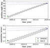 |
Fig. A.1. Astrometric proper motion analysis analog to Fig. 3, but for the additional wide-separation point source detected in the coronagraphic images. The astrometry in the SPHERE and NACO epochs is consistent with a non-moving (distant) background object. |
Appendix B: Randomly selected orbit plots
To illustrate the quality of the recovered orbit solutions in Sect. 6, we show, for both mass scenarios, ten randomly selected orbits. Astrometric data points are displayed in black.
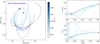 |
Fig. B.1. Ten random orbits for the low-mass scenario 1, that is, a system mass of 0.268 M⊙. On the left, we show the orbit in RA-Dec space and on the right, we show relative separation and position angle of the secondary relative to the primary versus time. |
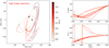 |
Fig. B.2. Ten random orbits for the high-mass scenario 2, i.e. a system mass of 0.42 M⊙. On the left, we show the orbit in RA-Dec space and on the right, we show relative separation and position angle of the secondary relative to the primary versus time. |
Appendix C: Cluster parallaxes
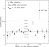 |
Fig. C.1. Parallaxes of known η Cha cluster members. ET Cha seems to be significantly closer than the other members. |
All Tables
Observing setup and average observing conditions for SPHERE/IRDIS and archival NACO observation epochs.
Astrometry and photometry of the ET Cha system, as extracted from our SPHERE/IRDIS observations as well as NACO archival data.
All Figures
|
Fig. 1. SPHERE/IRDIS and NACO observations of the ET Cha system. The companion is well-resolved in the 2019 SPHERE epoch. We note that we show the primary star on a slightly saturated color scale in order to highlight the companion (the data is not saturated). In the 2003 NACO epoch the companion is close to the resolution limit of the instrument and shows as a strong asymmetrical extension to the primary star PSF. We have performed a high-pass filter to make the companion more clearly visible. We mark the companion position in the NACO image by two white bars. |
| In the text | |
|
Fig. 2. Coronagraphic images of ET Cha taken with SPHERE/IRDIS in our program. Upper left: stacked total intensity image. Upper right: total intensity image after classical angular differential imaging reduction. Bottom: Stokes Q and U polarized flux images after polarization differential imaging. The size of the coronagraphic mask is indicated with the grey, hashed circle. The positive-negative signal pattern is caused by unresolved stellar polarization of the primary star, the companion or both and not by a resolved circumstellar disk. |
| In the text | |
|
Fig. 3. SPHERE/IRDIS and NACO astrometry of the detected companion relative to the primary star versus time. Position angle is measured from north over east. The grey ribbon shows the expected location of a non-moving background object, while the dashed lines indicate possible circular orbital motion assuming a face-on orbit for position angle and an edge-on orbit for separation independently (these are mutual exclusive orbits to illustrate the maximum expected change in separation and position angle for the circular case). |
| In the text | |
|
Fig. 4. Contrast limits derived from the coronagraphic observations using angular differential imaging and TLOCI post-processing. Mass limits for the 5 Myr and the 8 Myr case are indicated with the blue, dash-dotted lines and the red, dashed lines, respectively. |
| In the text | |
|
Fig. 5. Resulting orbit solutions for the ET Cha system using our extracted astrometry. We utilized the orbitize! package and the included OFTI algorithm with 106 generated orbits. We show semi-major axis, inclination, and eccentricity. Scenario 1 is in the lower left corner in blue color and scenario 2 is in the upper right corner in red. |
| In the text | |
|
Fig. A.1. Astrometric proper motion analysis analog to Fig. 3, but for the additional wide-separation point source detected in the coronagraphic images. The astrometry in the SPHERE and NACO epochs is consistent with a non-moving (distant) background object. |
| In the text | |
|
Fig. B.1. Ten random orbits for the low-mass scenario 1, that is, a system mass of 0.268 M⊙. On the left, we show the orbit in RA-Dec space and on the right, we show relative separation and position angle of the secondary relative to the primary versus time. |
| In the text | |
|
Fig. B.2. Ten random orbits for the high-mass scenario 2, i.e. a system mass of 0.42 M⊙. On the left, we show the orbit in RA-Dec space and on the right, we show relative separation and position angle of the secondary relative to the primary versus time. |
| In the text | |
|
Fig. C.1. Parallaxes of known η Cha cluster members. ET Cha seems to be significantly closer than the other members. |
| In the text | |
Current usage metrics show cumulative count of Article Views (full-text article views including HTML views, PDF and ePub downloads, according to the available data) and Abstracts Views on Vision4Press platform.
Data correspond to usage on the plateform after 2015. The current usage metrics is available 48-96 hours after online publication and is updated daily on week days.
Initial download of the metrics may take a while.