| Issue |
A&A
Volume 700, August 2025
|
|
|---|---|---|
| Article Number | A92 | |
| Number of page(s) | 21 | |
| Section | Cosmology (including clusters of galaxies) | |
| DOI | https://doi.org/10.1051/0004-6361/202449984 | |
| Published online | 08 August 2025 | |
TDCOSMO
XVIII. Strong lens model and time-delay predictions for J1721+8842, the first Einstein zigzag lens
1
Department of Physics and Astronomy, University of California, Los Angeles, CA 90095, USA
2
Department of Physics and Astronomy, Stony Brook University, Stony Brook NY 11794, USA
3
Kavli Institute for Particle Astrophysics & Cosmology, P.O. Box 2450 Stanford University, Stanford, CA 94305, USA
4
STAR Institute, Quartier Agora – Allée du six Août, 19c B-4000 Liège, Belgium
5
Technical University of Munich, TUM School of Natural Sciences, Department of Physics, James-Franck-Str 1, 85748 Garching, Germany
6
Max-Planck-Institut für Astrophysik, Karl-Schwarzschild-Str. 1, 85748 Garching, Germany
7
Department of Astronomy & Astrophysics, The University of Chicago, Chicago IL 60637, USA
8
Kavli Institute for Cosmological Physics, University of Chicago, Chicago IL 60637, USA
9
The Oskar Klein Centre, Department of Physics Stockholm University, SE – 106 91 Stockholm, Sweden
10
Institute of Physics, Laboratoire d’Astrophysique, Ecole Polytechnique Fédérale de Lausanne (EPFL), Observatoire de Sauverny, CH-1290 Versoix, Switzerland
11
European Southern Observatory, Alonso de Córdova 3107, Vitacura, Santiago, Chile
12
Institut de Ciències del Cosmos, Universitat de Barcelona, Martí i Franquès, 1, E-08028 Barcelona, Spain
13
ICREA, Pg. Lluís Companys 23, Barcelona E-08010, Spain
14
Center for Astronomy, Space Science and Astrophysics, Independent University, Bangladesh, Dhaka 1229, Bangladesh
⋆ Corresponding author: This email address is being protected from spambots. You need JavaScript enabled to view it.
Received:
14
March
2024
Accepted:
16
June
2025
Abstract
We present lens models for J1721+8842, the first-ever discovered galaxy-scale strong lens in an Einstein zigzag configuration. The model consists of four separate lensed galaxies, with the primary source hosting a quasar, lensed into six images by two deflectors at redshifts z1 = 0.184 and z2 = 1.885. The configuration of three lensed sources and the lensed light of the deflector at redshift z2 = 1.885 tightly constrain the mass profile of the primary lensing galaxy. Using two standard descriptions for the main perturber’s mass distribution – a total power-law profile and a composite dark and stellar mass – the inferred convergence around the location of the lensed images is in excellent agreement. While the strong lensing data alone does not significantly favor either of our profile assumptions for the main deflector’s mass distribution, we show that a central stellar velocity dispersion measurement can distinguish or validate them. Using a standard ΛCDM cosmology with H0 = 70 km s−1 Mpc−1, we present time-delay predictions between the lensed quasar images for both models at the percent level modulo a multiplane mass sheet transform. Our models are the first step toward constraining the time-delay distance ratios for J1721+8842, and thus also H0, independent of other methods. In order to achieve an H0 measurement, our models need to be combined in a multiplane lensing analysis with the stellar velocity dispersion for the deflectors, the line-of-sight convergence, and the observed time delays. Owing to its extraordinary configuration, this is an extremely promising system for a high-precision determination of H0.
Key words: gravitational lensing: strong / galaxies: elliptical and lenticular / cD / quasars: general / distance scale
NFHP Einstein Fellow.
© The Authors 2025
 Open Access article, published by EDP Sciences, under the terms of the Creative Commons Attribution License (https://creativecommons.org/licenses/by/4.0), which permits unrestricted use, distribution, and reproduction in any medium, provided the original work is properly cited.
This article is published in open access under the Subscribe to Open model. This email address is being protected from spambots. You need JavaScript enabled to view it. to support open access publication.
1. Introduction
The Hubble constant (H0), the current expansion rate of the Universe, is a quantity of fundamental importance in the current cosmological debate. The standard cosmological model based on cold dark matter (CDM) and a cosmological constant, Λ (hence ΛCDM), successfully matches a range of observations including the cosmic microwave background (CMB) radiation, the Big Bang nucleosynthesis, baryon acoustic oscillations (BAOs), galaxy clustering and the formation of large-scale structures, and measurements of Type Ia supernovae (SNIa) distances (e.g., Riess et al. 1998; Perlmutter et al. 1999; Eisenstein et al. 2005; Planck Collaboration VI 2020). Yet, in the flat ΛCDM, there is an increasing tension between the Hubble constant inferred from early Universe constraints and direct measurements using local Universe probes. For example, the analysis of anisotropies in the CMB result in H0 = 67.4 ± 0.5 km s−1 Mpc−1 (Planck Collaboration VI 2020) in a flat ΛCDM, whereas local measurements based on Cepheid variables and SNIa as rungs in the cosmic distance ladder give a Hubble constant of H0 = 73.04 ± 1.04 km s−1 Mpc−1 (Riess et al. 2022). The difference results in a tension of high statistical significance (see, e.g., Abdalla et al. 2022, and references therein). If independent methods confirm the tension is not caused by unknown systematic uncertainties in the measurements, then new physics beyond a flat ΛCDM model is required. Examples of proposed solutions include changing the sound horizon at recombination through a currently unknown relativistic particle or a form of early dark energy (see, e.g., Knox & Millea 2020; Di Valentino et al. 2021; Schöneberg et al. 2022; Vagnozzi 2023).
Strong gravitational lensing of a variable background source provides a powerful independent cosmological probe through which the Hubble constant can be measured in one step, thus bypassing the local distance ladder (Refsdal 1964; Treu & Marshall 2016; Treu et al. 2022; Treu & Shajib 2024; Birrer et al. 2024). Instead of relying on standard candles, strong lensing measures distances (and therefore H0) from the differences in the travel time of photons traversing the gravitational potential of the foreground deflector (see, e.g., Treu & Koopmans 2002; Suyu et al. 2010, 2014; Treu & Marshall 2016; Birrer et al. 2016; Bonvin et al. 2017; Birrer et al. 2019; Shajib et al. 2020).
One of the key ingredients of time-delay cosmography are accurate and precise gravitational lens models. In this paper, we present such models for the exceptionally complex gravitational lens system J1721+8842 (see Lemon et al. 2018, for discovery), the first-ever discovered galaxy-scale strong lens in an Einstein zigzag configuration (originally hypothesized by Collett & Bacon 2016). Using recent JWST observations, Dux et al. (2025) recently revealed that the system consists of a single active galactic nucleus at z = 2.36, producing six images as a result of compound lensing by two deflectors. The foreground lensing galaxy is located at redshift z = 0.184, and the deflector in between is at z = 1.885. This interpretation has been corroborated by the fact that all images measure the same redshift and that the light curves are identical within errors (Dux et al. 2025). This discovery renders the previous models by Mangat et al. (2021) and the automated models by Schmidt et al. (2023) and Ertl et al. (2023) obsolete.
This zigzag configuration is truly remarkable, as it not only places tight constraints on the distribution of mass in the primary deflector, but – compared to typical quadruply lensed quasars – the system also provides additional images and thus increases the set of measurable delays from 6 to 15 (or from 3 to 5 for a single reference image). The specific configuration also strongly constrains the overall gravitational optics of the systems, as the creation of six images requires a very tight alignment.
Our aim is to show that this configuration results in percent-level uncertainty in the predicted time delays within the context of the herein presented models. The final precision and accuracy will of course depend on breaking the multiplane mass-sheet degeneracy (MSD; Falco et al. 1985; Schneider & Sluse 2014; Schneider 2019), which will be discussed in a forthcoming paper (Millon et al., in prep.). However, the precision, number, and length (up to ∼200 days) of the predicted delays are crucial to breaking the MSD and demonstrating the tremendous potential of this Einstein zigzag for cosmography (for comparison, the most precise measurement to date reached a 3.9% precision on H0; Shajib et al. 2019).
We note that the lens model has been constructed without knowledge of the measured time delays, which are currently being derived and kept blind from this modeling effort. Stellar velocity dispersion and external convergence are also currently being measured. Once all ingredients are available, we will combine them with the relative Fermat potentials, given by our model, to determine the Hubble constant (H0) and other cosmological parameters. We note that the previous work by our collaboration has typically followed the reverse order, with a lens model being the final step (notable exceptions are the work by Shajib et al. 2022; Chen et al. 2022). For the purpose of determining H0, the order does not matter, and blindness can be imposed either way in order to prevent unconscious experimenter bias.
This paper is organized as follows. In Section 2 we summarize the theoretical background of strong gravitational lensing, discuss strong lens observables, and review the formal notation for the Bayesian framework used in our inference of time-delay predictions. Section 3 presents a description of the discovery of J1721+8842, the imaging of the target, and the data reduction. In Section 4 we discuss the individual components of our lens models and provide details on the parameterizations used in our analysis, including informative priors implemented to guide the results and the assessment of systematic uncertainties in the underlying choices for lens model components. The results of our analysis are presented in Section 5 along with measurable time-delay predictions between images pairs of the lensed quasar. Finally, Section 6 provides a brief summary. Whenever necessary, we used a cosmological concordance model with parameters H0 = 70 km s−1 Mpc−1, Ωm, 0 = 0.3, and ΩΛ, 0 = 0.7.
2. Modeling analysis
Our analysis uses Hubble Space Telescope (HST) imaging data, dHST, in three bands, UVIS (F475X and F814W) as well as IR (F160W), to make an inference on the lensing potential, ψ, for J1721+8842 and on the position of the lensed source, β. In addition to parameters for the mass model of the lens, ξmass, the HST observations further allowed us to obtain constraints on the parameterization of the surface brightness distribution for the primary deflector, ξlight, and for the lensed sources, ξsource.
In terms of organization, this section first gives a description of the strong lensing formalism and describes how our models connect to observables, presented in Section 2.1. We then discuss lensing degeneracies and potential sources of systematic uncertainties in Section 2.2, while Section 2.3 outlines the formal notation of the Bayesian inference used in our analysis.
2.1. Lensing theory and strong-lensing observables
Compared to a path without perturbation, the excess time-delay (see, e.g., Schneider et al. 1992; Blandford & Narayan 1992) for a lensed point source at position β = (β1, β2) in the source plane, observed at angular position θ = (θ1, θ2) in the lens (or image) plane, is described by
![Mathematical equation: $$ \begin{aligned} t(\boldsymbol{\theta }; \boldsymbol{\beta }) = \frac{D_{\Delta t}}{c} \left[\frac{(\boldsymbol{\theta }-\boldsymbol{\beta })^2}{2} - \psi (\boldsymbol{\theta }) \right], \end{aligned} $$](/articles/aa/full_html/2025/08/aa49984-24/aa49984-24-eq1.gif) (1)
(1)
where c is the speed of light, ψ(θ) represents the deflection potential of the lens, and whereby the time-delay distance, DΔt, is defined as
 (2)
(2)
with Dd, Ds, and Dds, as the angular diameter distance to the main deflector, to the lensed source, and between the source and the deflector, respectively. zd represents the redshift of the lensing galaxy.
The delay in the arrival time of photons emitted by the same source, but observed at two different positions in the image plane, θA and θB, can then be expressed as
 (3)
(3)
where ΔϕAB is the difference in the Fermat potential, ϕ(θA; β)−ϕ(θB; β), between the two image positions, with the Fermat potential defined as
 (4)
(4)
With that definition,
![Mathematical equation: $$ \begin{aligned} \Delta \phi _{\mathrm{AB}}(\boldsymbol{\theta _{\mathrm{A}}}; \boldsymbol{\theta _{\mathrm{B}}}; \boldsymbol{\beta }) = \frac{1}{2} \left[ (\boldsymbol{\theta _{\mathrm{A}}} - \boldsymbol{\beta })^2 - (\boldsymbol{\theta _{\mathrm{B}}} - \boldsymbol{\beta })^2\right] - \left[ \psi (\boldsymbol{\theta _{\mathrm{A}}}) - \psi (\boldsymbol{\theta _{\mathrm{B}}}) \right], \end{aligned} $$](/articles/aa/full_html/2025/08/aa49984-24/aa49984-24-eq5.gif) (5)
(5)
where the first difference is the geometric term as the result of the light traversing paths of different lengths due to different deflection angles at the corresponding image positions, while the second term describes the difference in the gravitational delayphotons experience while traveling through the potential of the lensing galaxy.
The deflection angle, α(θ), at an image position, θ, can be expressed as the gradient of the deflection potential, α(θ) = ∇ψ(θ), and is dictated by the lens equation, β = θ − α(θ), which describes the lensing of a source at position β by the deflection potential, ψ(θ). In the limit of the deflector mass being confined to a two-dimensional sheet (the lens plane) with a physical projected surface mass density, Σ(θ), (the thin lens approximation), the deflection angle is related to the dimensionless projected surface mass density, or convergence, κ, by
 (6)
(6)
where κ(θ) is defined as the surface mass density scaled by the critical surface mass density, κ(θ)≡Σ(θ)/Σcr, with
 (7)
(7)
Therefore, the dimensionless convergence is related to the deflection potential of the lensing galaxy by
 (8)
(8)
High-resolution observations, taken with the Hubble Space Telescope, allow us to constrain the deflections potential, ψ, along with the unknown position of the lensed source, β, by constructing models that match the lensed positions of a multiply imaged background quasar. Furthermore, if the source galaxy hosting the lensed quasar is bright and spatially extended, the arc of the lensed background source provide additional constraint to distribution of the lensing potential. Together with measured time delays, Δt, for the image positions, the Fermat potential difference between two images is used to infer the time-delay distance, DΔt, which is inversely proportional to the Hubble constant, DΔt ∝ H0−1.
2.2. Lensing degeneracies
Strong gravitational lens models suffer from a number of well-known parameter degeneracies, whereby various combinations of distinct parameters produce different models that fit the observed data (see, e.g., Saha 2000; Saha et al. 2006). One of the fundamental degeneracies in strong lens modeling is the mass-sheet degeneracy, or MSD, (see, e.g., Falco et al. 1985; Schneider & Sluse 2014), which refers to the fact that a model’s convergence, κ, can be transformed by a constant factor, λ, such that observable quantities such as image positions and flux ratios remain unchanged if the unknown source position, β, is rescaled by the same factor, i.e.
 (9)
(9)
Mathematically, this mass sheet transformation (MST) corresponds to an addition of a uniform sheet of mass that changes the convergence term, but not the shear, while simultaneously re-scaling the angular distances.
It should be noted that the true physical convergence of the lens system, κphys(θ), has two main components, namely the convergence associated with the primary deflector and neighboring galaxies, κint(θ), thereby influencing the stellar kinematics of the lens galaxy, as well as an external convergence, κext, physically associated with the perturbation from line-of-sight structure, meaning
 (10)
(10)
However, the spatial extent of the lens galaxy, and with it the gravitational influence, is limited; therefore the convergence intrinsically associated with the main deflector is physically constrained to a certain radial span. In other words, the internal convergence vanishes at large radii, i.e. limθ → ∞κint(θ) = 0, which implies that at a large distance away from the primary perturber the total physical convergence of the system is attributed entirely to the external convergence, i.e. limθ → ∞κphys(θ) = κext.
At this point, the convergence of any lens model, κlens(θ), can itself be thought of as a transformation of the lens system’s physical convergence, κphys(θ), so
 (11)
(11)
During the modeling of the primary lens, however, the line-of-sight contribution to the convergence is commonly omitted, which means the convergence of the lens model, κlens(θ), does not include the external convergence term, κext. Therefore, if we combine Expression (10) with Expression (11), then in the limit of θ → ∞, we have 0 = λ(0 + κext)+(1 − λ), which arranged for λ, simplifies to
 (12)
(12)
We can now use Expression (12) together with Expression (10) in Expression (11) to arrive at
![Mathematical equation: $$ \begin{aligned} \kappa _{\mathrm{lens}}(\boldsymbol{\theta }) = \frac{1}{1-\kappa _{\mathrm{ext}}} \left[ \kappa _{\mathrm{int}}(\boldsymbol{\theta }) + \kappa _{\mathrm{ext}} \right] + \left(1 - \frac{1}{1-\kappa _{\mathrm{ext}}}\right), \end{aligned} $$](/articles/aa/full_html/2025/08/aa49984-24/aa49984-24-eq13.gif) (13)
(13)
which in terms of κint(θ) simplifies to
 (14)
(14)
All reconstructed models presented in this paper employ parameterized profiles, which mitigate the impact of the MSD on the convergence of such a model. In other words, the convergence of a lens model, κlens(θ), would be a transformation of such a parameterized model, κparam. In the absence of the external convergence term, the MST (Expression (9)) is
![Mathematical equation: $$ \begin{aligned} \kappa _{\mathrm{lens}}(\boldsymbol{\theta }) = \lambda _{\mathrm{int}}(\boldsymbol{\theta }) \kappa _{\mathrm{param}}(\boldsymbol{\theta }) + \left[1 -\lambda _{\mathrm{int}}(\boldsymbol{\theta }) \right]. \end{aligned} $$](/articles/aa/full_html/2025/08/aa49984-24/aa49984-24-eq15.gif) (15)
(15)
Lastly, combining Expression (15) with Expression (14) and using the result in Expression (10) gives the following expression for the real physical convergence of the lens system in terms of a parameterized profile:
![Mathematical equation: $$ \begin{aligned} \kappa _{\mathrm{phys}}(\boldsymbol{\theta }) = (1-\kappa _{\mathrm{ext}}) \left[ \lambda _{\mathrm{int}}(\boldsymbol{\theta }) \kappa _{\mathrm{param}}(\boldsymbol{\theta }) + 1-\lambda _{\mathrm{int}}(\boldsymbol{\theta }) \right] + \kappa _{\mathrm{ext}}, \end{aligned} $$](/articles/aa/full_html/2025/08/aa49984-24/aa49984-24-eq16.gif) (16)
(16)
which simplifies to
![Mathematical equation: $$ \begin{aligned} \kappa _{\mathrm{phys}}(\boldsymbol{\theta }) = \lambda (\boldsymbol{\theta }) \kappa _{\mathrm{param}}(\boldsymbol{\theta }) + \left[1-\lambda (\boldsymbol{\theta })\right], \end{aligned} $$](/articles/aa/full_html/2025/08/aa49984-24/aa49984-24-eq17.gif) (17)
(17)
where
 (18)
(18)
Kinematic measurements, such as the stellar velocity dispersion in the primary deflector near the image positions, can be used in conjunction with corresponding mass estimates from strong lens models to break the degeneracy internal to the lens galaxy and thereby constrain the internal MST parameter, λint(θ). An estimate for the external convergence, κext, can be obtained from environmental studies of the lens system, such as spectroscopic and photometric surveys which provide redshifts as well as a quantification for the perturber population along the line of sight.
As a consequence of the MSD, it should be noted that the expression for the Fermat potential (Expression (4)) also re-scales under the MST with
 (19)
(19)
However, in the vicinity of the observed image positions, λint(θ) is nearly invariable, so that λ(θ)→λ = λint(1 − κext). Therefore, the Fermat potential difference between two images A and B for the true physical convergence scales with the Fermat potential difference of the reconstructed parameterized model as
 (20)
(20)
In short, both, a measurement for the external convergence, κext, and the scale factor internal to the lens galaxy, λint, near the image positions, are needed to make an inference of the Hubble constant using observations of strongly lensed quasars.
One important caveat to note is that because of its multiplane nature, J1721 is less sensitive to the MST than standard lenses (e.g., Schneider & Sluse 2014), and therefore one will have to consider the effects of the MSD in a multiplane framework when deriving cosmological constraints. The analysis presented in this paper does not account for the additional constraint imposed by the possible range of mass sheet transformations, but this work is left for a future investigation in Millon et al. (in prep.).
2.3. Bayesian analysis and likelihood
The aim of this analysis is to obtain posterior distributions for the parameters, ξ, of a model, M, given the data set from the HST observations, dHST. Using Bayes’ theorem, we can express the probability of the model parameters as
 (21)
(21)
where in the last step we have broken up the set of model parameters into the main components of a lens model; namely the parameters of the deflector mass, ξmass, the parameters for the light profile of the deflector and the lensed source, ξlight and ξsource, respectively, and the model for the point spread function, 𝒫.
The posterior of a single attribute in the lens model, ξi, which is part of the set of all model parameters, can then be determined by marginalizing over the remaining (nuisance) parameters, ξk:
 (22)
(22)
It should be mentioned that not all models in this paper share the same parameters. Therefore, to substantiate a meaningful comparison between various models and to determine which model best matches our observations, we use the Bayesian information criterion, which is defined as
 (23)
(23)
where k is the number of all free and linear parameters in a model, n represents the number of data points (or pixels), and  stands for the maximum value of the likelihood function, P(dHST|ξ, M), corresponding to the model.
3. Observations of lens system J1721+8842
In this section we discuss the discovery of J1721+8842 in Section 3.1. We also describe the target’s observations as well as the imaging data reduction in Section 3.2.
3.1. Lens discovery and redshift measurements
Originally discovered by Lemon et al. (2018) through a search for multiple Gaia detections around potential quasars, this system is confirmed to be a strongly lensed quasar with a redshift of z ≈ 2.37, showing strong absorption features. Lemon et al. (2022) interpreted the system as the result of two distinct background quasars at similar redshifts (z = 2.369 ± 0.007 and z = 2.364 ± 0.003), with one quasar quadruply imaged and the other doubly imaged. This interpretation is now rendered obsolete by the information that became available later, identifying the Einstein zigzag configuration. Furthermore, the images A and C of the quadruply lensed quasar exhibit damped Lyman-α absorption signatures from neutral hydrogen at a redshift consistent with the measurements for the quasars.
The long-slit spectra of the lensing galaxy, obtained with the Intermediate-dispersion Spectrograph and Imaging System at the William Herschel Telescope, show multiple absorption features stemming from Ca H and K in the G-band, as well as Mg, Na, and Hβ. Fitting these lines with a multi-component Gaussian, Lemon et al. (2022) estimate the redshift of the deflector to be z = 0.1841 ± 0.0005. Lastly, the source is also detectable at radio wavelengths (see Mangat et al. 2021).
Follow-up observations with the James Webb Space Telescope (JWST) Near InfraRed Spectrograph (NIRSpec; GO-2974; PI Treu; co-PI Shajib) have revealed the supposed host of the previously assumed doubly imaged quasar (see Mangat et al. 2021) to be another deflector at a redshift of z = 1.885, resulting in a six-image configuration of a single quasar lensed by two galaxies nearly perfectly aligned along the line of sight. Further evidence in support this Einstein zigzag configuration is demonstrated by the within-error identical light curves for the images of the previously believed quadruply and doubly imaged quasars (see Dux et al. 2025).
We also extracted the spectra for S3 and S4 from the NIRSpec data cube, which was centered on the lensing galaxy, placing S3 and S4 on the edge of the spectrograph. Still, these two sources extend over a few pixels within the NIRSpec field of view, allowing us to measure their redshift. From the detection of the Hβ, [OII]λ 3727Å, [OIII]λ 4959 Å and [OIII]λ 5007 Å, we confirm that theses sources are at the same redshift as the quasar, i.e. z = 2.38.
3.2. HST imaging and data reduction
The high-resolution data for this lens comes from observations with the Hubble Space Telescope, taken under cycle 26 program HST-GO-15652 (PI: T. Treu; see Schmidt et al. 2023), using the Wide Field Camera 3 (WFC3). Our dataset comprises imaging in filter F160W, to give near-IR modeling constraints, and UVIS exposures in band F475X and band F814W, for higher-resolution observations in the optical/UV spectrum. In the IR band, a 4-point dither pattern is employed to improve the data sampling by eliminating hot pixels and other detector irregularities, while UVIS exposures implement 2-point dithering during observations. At each UVIS dither point exposures are split into one long and one short integration to ensure the full brightness span is captured between faint features of the lens and bright quasar images. The total integration time for the four IR exposures is 2197 s, whereas the exposure time in the UVIS totals 1382 s in filter F475X and 1428 s in filter F814W.
Cosmic ray hits are removed and the individual exposures in each filter are aligned and combined with the use of the Python package ASTRODRIZZLE (Avila et al. 2015). The resulting reduced images have a pixel size of 0.04″/pix in both UVIS bands and 0.08″/pix for the IR imaging. A composite red-green-blue image of the target, constructed from the reduced IR/UVIS exposures, is shown in Figure 1, identifying the lens, nearby perturbing galaxies, and the deflector at redshift z = 1.885. Figure 2, labels the images of lensed quasar and other lensed sources. The intensities for each channel in the color composites are entirely arbitrary and chosen to achieve the best visualization of all components in the lens system.
 |
Fig. 1. Red-green-blue composite image of J1721+8842 and nearby perturbers created by exposures in the HST band F160W (red), F814W (blue), and F475X (green). |
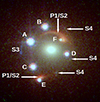 |
Fig. 2. Red-green-blue composite image of J1721+8842 created by exposures in the HST band F160W (red), F814W (blue), and F475X (green). |
4. Lens models
In this section we describe the modeling choices for all components in the lens models of J1721+8842, broken down between main deflector description, lensed source light components, explicitly modeled line-of-sight perturbers, and structure resulting in additional distortions to the lens configuration. The parameterizations of the main deflector’s mass profiles are discussed in Section 4.1.1, while the parameterization of the light profiles corresponding to the primary lensing galaxy are described in Section 4.1.2. The light profiles of the lensed sources and quasar, including the light profile for the deflector at redshift z = 1.885, are discussed in Section 4.2 and the modeling choices related to all additional perturbing galaxies are outlined in Section 4.3. After that we describe the parameterization of LOS model components in Section 4.4, show assumed priors for specific parameters in Section 4.5, and conclude with a discussion on modeling choice related systematics in Section 4.6.
4.1. Main deflector
4.1.1. Main deflector mass profile parametrization
For the main deflector, we use two independent modeling choices (or “modeling families”) to parameterize the mass profile. Option 1 relies on a singular power-law elliptical mass distribution to model the main deflector mass (see Power-law mass profile paragraph) while for option 2 the mass of the deflector is modeled as a composite profile, where we separate the deflector’s dark matter component from the luminous baryonic matter (Composite mass profile paragraph).
4.1.1.1. Power-law mass profile.
In this choice for parametrization, the mass profile of the main deflector is modeled with a power-law elliptical mass distribution (PEMD), which corresponds to a radial mass density profile of ρ ∝ r−γ, where γ is the power-law slope. The convergence, or dimensionless projected surface mass density, for the profile at position θ is parameterized as
 (24)
(24)
where θ1 and θ2 are aligned along the semi-major and semi-minor axis through the rotational position angle ϕ = arctan(θ2, qθ1), and where q represents the corresponding axis ratio. The centroid of the main-delfector’s mass model is linked to the corresponding light profile through a maximum allowed offset of 2 pixels as well as a Gaussian prior with a variance of 1 pixel, which corresponds to  in UVIS.
4.1.1.2. Composite mass profile.
For the parametrization of this modeling option, we use two separate mass profiles: one to model the dark matter component of the main deflector mass and another profile to represent the baryonic matter. For the dark matter component, we adopt an spherical Navarro–Frenk–White (NFW) profile, for which the three dimensional mass density is given by
 (25)
(25)
where ρ0 is the normalization constant and r0 represents the scale radius (Navarro et al. 1997). Further details on the convergence and lensing potential of the NFW profile can be found in (Golse & Kneib 2002).
The luminous baryonic matter of the main deflector mass is modeled by two elliptical chameleon convergence profiles, which are superposed and joined via a common centroid. This mass profile is further tied to light profile model of the F160W IR band (see Section 4.1.2). The convergence of a chameleon profile is given by the difference between two non-singular isothermal ellipsoids with different core sizes and is parameterized as
![Mathematical equation: $$ \begin{aligned} \kappa (\theta _1, \theta _2)&= \frac{\kappa _0}{1 + q} \left[ \frac{1}{\sqrt{\theta _1^2+\theta _2^2/q^2 + 4w_{\rm c}^2/(1+q^2)}} \right.\nonumber \\&\quad \left. - \frac{1}{\sqrt{\theta _1^2+\theta _2^2/q^2 + 4w_{\rm t}^2/(1+q^2)}} \right] , \end{aligned} $$](/articles/aa/full_html/2025/08/aa49984-24/aa49984-24-eq28.gif) (26)
(26)
where wc and wt are the profile parameters for the two core sizes, where κ0 represents the normalization constant, and where q is again the corresponding axis ratio (Dutton et al. 2011; Suyu et al. 2014). In contrast to a Sérsic profile, the chameleon profile is based on closed-form expressions and thereby proofs more convenient in the computation of lensing quantities (see Suyu et al. 2014). Furthermore, within a radius of between 0.5 Re and 3.0 Re, where Re is the effective radius of the Sérsic profile, the chameleon profile approximates the Sérsic profile to within a few percent in mass residuals (Dutton et al. 2011).
As additional constraint to the composite mass profile parameterization, we force a common centroid between dark matter and baryonic matter components. This is achieved by allowing the centroid of the NFW profile to be offset from the double chameleon profile centroid by at most by 1 pixel, which corresponds to  in UVIS, and effectively joins the centroids of the two mass profiles.
4.1.2. Main deflector light profile parameterization
Analogous to Section 4.1.1, we use two modeling choices to parameterize the light profile of the main deflector, which depend on the deflector’s mass profile parameterization. If the deflector’s mass profile is described by a power-law, we model the main deflector light with Sérsic profiles, which is detailed in Section 4.1.2. In the composite mass profile case (Section 4.1.2), we used a chameleon or Sérsic light profile parameterization, depending on the filter in which the target wasobserved.
4.1.2.1. Light profile parameterization to power-law mass profile.
In the case of the power-law mass profile modeling choice, we use a Double Sérsic profile (Sérsic 1968) with a common centroid to model the light of the main deflector in all three bands. The parameterization of an elliptical Sérsic light profile is given by
![Mathematical equation: $$ \begin{aligned} I(\theta ) = I(\theta _{\mathrm{e}}) \, \exp \left\{ -C(n) \left[ \left( \frac{(q_{\mathrm{L}}\theta _1)^2 + \theta _2^2}{q_{\mathrm{L}}\theta _{\mathrm{e}}^2} \right)^{\frac{1}{2n}} -1 \right] \right\} , \end{aligned} $$](/articles/aa/full_html/2025/08/aa49984-24/aa49984-24-eq30.gif) (27)
(27)
where C(n) is a normalization constant so that at the effective radius, θe, the profile includes half of the deflector’s light. n represents the Sérsic index, θ1 and θ2 are the angular coordinates aligned along the semi-major and semi-minor axis through the rotational position angle ϕL = arctan(θ2, qθ1) of the light profile, and qL represents the corresponding axis ratio. In our models we hold the index of the first Sérsic light profile fixed at n = 1.0 across all filters, effectively making it an exponential Sérsic profile. The Sérsic index of the second light profile is allowed to vary within the restrictions of a flat prior as discussed in Section 4.5. Additionally, we allow the effective radii, the Sérsic index of the second light profile, the axis ratios, the position angles, and the centroids to vary across bands.
4.1.2.2. Light profile parameterization to composite mass profile.
For the composite mass profile option, we model the main deflector light with Double Sérsic profile (Expression (27)) in the UVIS bands (filters F475X and F814W), as described above in Section 4.1.2. However, in the IR band (filter F160W), the paramerterization of the deflector light is following the description of the profile representing the baryonic matter, where we model the main deflector with two joined elliptical chameleon profiles, shown in Expression (26). For the light profile description, however, we replaced the normalization constant, or convergence amplitude, κ0, by the normalization constant for the flux amplitude, I0. The remaining parameters of Expression (26) remain the identical and are all tied (or held in common) between the double chameleon mass and light profiles.
4.2. Lensed sources
4.2.1. Quasar host galaxy
The galaxy hosting the sextuply imaged quasar is modeled with an elliptical Sérsic light profile (see Expression (27)). Except for the centroids, which are held common across the three HST bands, all parameters for the Sérsic profiles are allowed to vary independently and are constrained by the flat priors described in Section 4.5. To model additional complexity in the source light, which cannot be described by a continuous or featureless flux distribution of a Sérsic profile, we add a set of two-dimensional Cartesian shapelets (Refregier 2003; Birrer et al. 2015) to the light profile of the host galaxy. These shapelets share a common centroid with the Sérsic function of the associated host. The corresponding number of basis functions (or shapelet number) form an orthogonal basis and is given by
 (28)
(28)
where the maximal source complexity, or nmax, is related to the characteristic scale, β, by the maximum spatial scale, lmax, defined as
 (29)
(29)
Increasing the shapelet order, nmax, increases the complexity, or components of additional concentrated flux, in the source reconstruction of our models. To prevent the shapelet order from being driven to high values, which would result in degeneracies with other model parameters and further cause overfitting by modeling noise in the data, we kept the parameter nmax for each band fixed during the fitting process for a given model and only allowed the scale size, β, to vary within the confines of a flat prior.
The multiply imaged quasar hosted by the lensed galaxy is modeled as point source in the image plane and shares the same centroid as the associated host in the source plane. To account for the lower resolution in the IR band (F160W), the point spread function (PSF) is supersampled in IR using a supersampling factor of 3. For the two UVIS bands, however, we do not use a supersampled PSF. As initial starting point we first estimate the PSF in each band using 5–10 suitable stars in the field of view near the target. Then, to further refine and improve the PSF, we run iterations of the PSF reconstruction between optimization routines that fit the free parameters for the respective lens model (see Birrer et al. 2019).
4.2.2. Lensed galaxies
Analogous to the quasar host, additional lensed sources, including the light of the deflector at redshift z = 1.885, are parameterized in our models by an elliptical Sérsic light profile as described by Expression (27). As the case with the quasar host galaxy, detailed in Section 4.2.1, only the centroids are joined across all bands for each source light profile, while all other parameters, such as ellipticity, Sérsic index, and Sérsic radius, are allowed to vary within the confines of the respective prior (see Section 4.5). If additional complexity is required to accurately describe the lensed source light, we use the two-dimensional Cartesian shapelet profile, outlined in Section 4.2.1 above, with the centroid joined to the respective Sérsic profile to further model concentrated flux features. Again, only the scale size, β, is allowed to vary while the shapelet order, nmax, responsible for an increase in source complexity with larger values, is held fixed during the fitting process.
4.3. Additional perturbing galaxies
Galaxies near the main deflector and, in general, galaxies along the line of sight, can have a significant impact on the path of lensed quasar’s light rays, depending on the strength of their deflection potential and the perturber’s location with respect to the lens galaxy. Therefore, to ensure that higher order lensing effects beyond external convergence and external shear or flexion are properly addressed, we explicitly include certain line-of-sight perturbers in our models. In Section 4.3.1 we detail how we select nearby pertubers that are explicitly included in our models, followed by the description of the mass profile for modeled line-of-sight galaxies (Section 4.3.2).
4.3.1. Selection of nearby perturbers explicitly included in models
To determine which of the nearby perturbers should be explictly included (or explicitly modeled) in the plane of the main deflector, we use an estimate of the change in flexion produced by the perturbing galaxy. It should be noted that the perturber at redshift z = 1.885 is already deemed to be explicitly included in our models in a separate redshift plane and is therefore omitted from the flexion shift assessment.
The magnitude of the flexion shift caused by a perturber of assumed point mass is given by
 (30)
(30)
where θE and θE, p are the Einstein radius of the main deflector and the perturber, respectively (see Sluse et al. 2017; McCully et al. 2017). θ represents the angular separation between the perturber and the main deflector in the sky and the factor f(η) is defined as follows:
 (31)
(31)
where
 (32)
(32)
Ddp, Ds, Dp, and Dds represent the angular diameter distances between the redshifts of the main deflector and the perturber, to the source, to the perturber, and between the deflector and the source, respectively.
At the time of our analysis redshift measurements for nearby perturbers are not available. Given that the additional galaxies in the field-of-view and the main deflector are similar in color, we make the simplifying assumption that all are part of the same galaxy overdensity and therefore at approximately the same redshift. With this assumption η goes to zero and the function f(η) becomes unity, leaving the flexion shift magnitude at
 (33)
(33)
Under the assumption of an isothermal profile, the Einstein radius of an additional perturber is given by
 (34)
(34)
where Dps and Ds are the angular diameter distance between redshifts of the perturber and the lensed source and the angular diameter distance to the source, respectively. Using the Faber-Jackson (Faber & Jackson 1976) relation, L* ∝ σγ, which relates the velocity dispersion, σ, to the stellar luminosity, L*, with the power-law index, γ, equal to 4, we scale a perturbers’s Einstein radius to the corresponding flux, F, as
 (35)
(35)
Since we assume the perturbers to be in the same redshift plane as the main deflector, we have an expression for the Einstein radius based on the flux ratio:
 (36)
(36)
where Fp is the flux of the perturber and Fd the flux of the main deflector. Using Expression (36) in Expression (33), the estimated flexion shift magnitude produced by a perturber at the same redshift as the main deflector is then
 (37)
(37)
The flexion shift based on our flux ratio analysis for each perturber is listed in Table 1. As demonstrated in McCully et al. (2017), to prevent a significant bias in an H0 measurement line-of-sight perturbers which produce a flexion shift magnitude of Δ3x > 10−4 arcsec should be explicitly included in the lens models. Adopting this conservative cutoff, we find that pertuber P4 is located at a large enough angular separation for its impact to be negligible. In contrast, even though perturbers P5 and P6 have smaller angular scales compared to other nearby galaxies, their close proximity to the main deflector warrants their explicit inclusion in the lens models. Therefore, we include mass profiles to model perturbers P2, P3, P5, and P6, located in the same redshift plane as the main deflector, for our lens models.
Flexion shift estimates for nearby perturbers based on a corresponding flux ratio analysis.
4.3.2. Mass profile of nearby perturbers
Any additional perturbing galaxy, namely the deflector at redshift z = 1.885 as well as galaxies near the main deflector, deemed to be explicitly included in our models based on the criteria described in Section 4.3.1, is modeled using a singular isothermal sphere (SIS) profile, which represents a PEMD with a fixed power-law slope, γ, of 2.0 and a fixed axis ratio, q, of 1.0. For the pertubers located in the plane of the main deflector we fix the location of the mass centroid in our models to coincide with the corresponding light centroid that is used to measure the angular separation from the main perturber. As for the deflector at redshift z = 1.885, we link the mass centroid with the centroid of the corresponding Sérsic profile modeling the perturber’s light distribution as described in Section 4.2.2.
In the case of the perturbers in the main deflector plane, namely perturbers P2 through P6, we further employ a Gaussian prior on the Einstein radius that is based on an assumed 0.1 dex scatter in the Faber-Jackson relation (see Equation (35)). Furthermore, due to the complexity of the model and the underlying degeneracy for nearby line-of-sight perturbers, we hold Einstein radius for all the additional perturbers fixed at the estimates derived from the measured flux ratios (Equation (36)) until we find a good fit for all other parameters. Once a fit for the remaining parameters in our model is found, we add the Einstein radii back to the list of free parameters fit in the modeling process.
4.3.3. Light profile of nearby perturbers
With the exception of the deflector at redshift z = 1.885, for which the modeled light profile is described in Section 4.2.2 above, which covers the treatment of additional lensed galaxies, the light profiles for additional perturbing galaxies are not included in our models as they do not contribute valuable information toward the assessment of the Fermat potential differences between the image positions of the lensed quasar.
4.4. Line of sight structure and higher-order distortions
Additional linear distortions can impact the lens model as a result of dark matter halos and large scale structures along the line of sight. We collectively account for such an impact on the strong lens by including an external shear profile. The external shear strength of the combined tidal effect from the surrounding gravitational field is given by
 (38)
(38)
where the components of the external shear matrix, γext, 1 and γext, 1, are related to the external shear angle, ϕext, by
 (39)
(39)
4.5. Priors
This section provides details on the priors employed in the modeling process, which crucially quantify the intrinsic flexibility afforded to our lens models during parameter optimization. These informative constraints encapsulate observational and theoretical guidance toward realistic ranges in model parameters. The majority of parameters in our models rely on uniform priors that cover a broad physical range, with the exception of the NFW profile, in our composite model, and the Einstein radii of explicitly included nearby perturbers.
In addition to a flat prior, the centroid of the dark matter profile (NFW) is further constrained by the centroid of the chameleon profile. To effectively link the centers of the two profiles, we allowed for a deviation within the right ascension and declination of 1 pixel in UVIS, or 0 04. If for a model the NFW centroid exceeds the bound set by the chameleon profile, a taxing punishment term is added to the model’s likelihood. To constrain the scaling radius (r0) of the NFW profile we employ a Gaussian prior, which was derived using the analysis in Gavazzi et al. (2007) of Sloan Lens ACS (SLACS) lenses (see Bolton et al. 2006). Our prior for the scaling radius is centered on
  with a standard deviation of
  . When applying the prior on r0, we only probe the space within 5σ of the mean, meaning from
  to
to  , and disregard all solutions outside that range. Lastly, due to a degeneracy with the external shear parameters and associated convergence issues, we opted to employ a spherical NFW profile rather than punishing the likelihood of models with excessive results for eccentricity parameters.
Explicitly modeling four of the nearby perturbers, P2 through P6, further increases the already high complexity of our models. Furthermore, two of these perturbers are located near each other and thereby introduce additional degeneracies. For this reason, we impose a Gaussian prior on the Einstein radii of each explicitly included perturbing galaxy, with the exception of the deflector at redshift z = 1.885, and hold the mass centroid fixed at the corresponding center of light. The mean for the priors on the Einstein radii is derived using the flux ratio analysis in Expression (36) and the standard deviation is estimated based on a 0.1 dex scatter we assumed for the Faber-Jackson (Faber & Jackson 1976) relation. We show the resulting probability density for each prior on the perturber’s Einstein radius in Figure 3.
 |
Fig. 3. Priors on Einstein radii for nearby perturbing galaxies explicitly included in the models. |
Finally, in Table 2 we summarize the priors employed in our models by component. In case of non-spherical profiles, instead of listing the priors for axis ratio, q, and position angle, ϕ, we show the priors imposed on the corresponding eccentricity parameters, which are related to the axis ratio and position angle by
 (40)
(40)
Priors on mass model parameters.
4.6. Assessment of systematic uncertainties from modeling choices
To assess the systematic impact of various parameter choices on the uncertainties in our models, we model the lens configuration under different assumptions for the mass profile of the primary deflector and with three separate sets for radius of the circular mask used for the likelihood computation. The size of the likelihood masking region in our fiducial models is chosen to encompass a region large enough to ensure all lensed features are included within and to capture the extend of the primary deflector’s flux in each band. To test the impact of the likelihood masking size we increase and decrease the radius for each filter by  for our fiducial models and repeat the MCMC sampling procedures. We find no significant change in the time-delay difference between images as a result of these masking size changes and therefore opted to reduce the change in masking radii to
  for our remaining systematic assessments.
We further evaluate the impact of various complexities in the lensed sources by changing the shapelet order, nmax. Here, the lowest possible source complexity is represented by nmax = −, which signifies no shapelets were added to the source light modeled by a Sérsic light profile.
To obtain posteriors for the changes in parameter choices, we initialize the changed model with the results of the corresponding fiducial model for main deflector profile choice (the seed) and run the MCMC sampling procedure with an iteration count similar to the seed model. To summarize our selections, the changes to the model configurations, itemized by modeling component, are as follows:
-
Two choices for the mass profile of the primary deflector:
-
Power-law profile
-
Composite profile
-
-
Three choices for the radius (in arcsec) of the likelihood computation masking region, sorted by band from shortest to longest wavelength, i.e. {F475X, F814W, F160W}:
-
{3.9, 4.0, 7.4}
-
{4.0, 5.0, 7.5}
-
{4.1, 5.1, 7.6}
-
-
Complexity in lensed source light (nmax values), sorted by source number, i.e. {S1, S2, S3, S4}:
-
{−, 2, −, 5}
-
{−, 4, −, 7}
-
{−, 4, 1, 7}
-
{1, 4, 1, 7}
-
Combining these choices in modeling components, we arrive at a total of 24 different configurations. To address stochasticity in the MCMC sampling, we performed the MCMC run for each model configuration two times, which increases the number of model results contributing in the assessment of systematic uncertainties to a total of 48.
5. Results
We now present the reconstructed models for J1721+8842. In Section 5.1 we show the best fits for the profile parameters used in our modeling and discuss noteworthy findings. Section 5.2 describes how results for model of different complexities and components are compared to one another and Section 5.3 presents predicted time delays between lensed images based on the fits for our best models.
5.1. Lens model results
Figures 4 and 5 compare the reconstructed model with the data in each band. The first column in these figures shows the observations, ordered in terms of wavelength from short to long, i.e. filter F475X (top row), F814W (middle row), and F160W (bottom row). The second column presents the reconstructed model for a corresponding filter, while the third column shows the normalized residuals after subtracting the observations from the modeling results of each band.
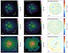 |
Fig. 4. Reconstructed power-law model for J1721+8842. The first column (left) shows the observations in each band, sorted by wavelength from short to long. The second column (center) displays the reconstructed model for each filter, and in the third column (right) are the normalized residuals between our model and the observed data. |
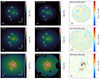 |
Fig. 5. Reconstructed composite model for J1721+8842. The first column (left) shows the observations in each band, sorted by wavelength from short to long. The second column (center) displays the reconstructed model for each filter, and in the third column (right) are the normalized residuals between our model and the observed data. |
In the corner plot of Figures 6 and 7, we show the posterior distributions for mass model parameters of both assumptions for the primary deflector’s profile, power-law (shown in red), and composite models (shown in blue) along with time delays between image pairs AD, AE, and AF of the sextuply lensed quasar. To compare the results of the composite model with the results of the power-law assumption, we show the Einstein radius, θE, for the composite model as radius of the circularized profile at which the encompassed mean convergence equals unity. In the same fashion, the power-law slope, γ, for the composite assumption is then computed from the derivative of the corresponding convergence profile at the Einstein radius.
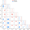 |
Fig. 6. Mass model parameters and predicted time delays for the two underlying assumptions of the primary deflector’s mass profile. The power-law model results are shown in red while the results for the composite model are colored in blue. In the composite model case, the Einstein radius of the main deflector, P0, is calculated via the circularized average of the convergence and the power-law slope represents the derivative of the convergence at the Einstein radius. To address computational challenges in sampling the composite model parameter space, the external shear is held fixed at the power-law model results, and therefore no composite model posteriors are shown. |
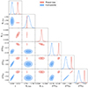 |
Fig. 7. Power-law slope, Einstein radii for both deflectors, P0 (main deflector) and P1, and predicted time delays for the two mass profile assumptions of the main deflector. The power-law and composite model results are shown in colors red and blue, respectively. In the composite model case, the Einstein radius of the main deflector, P0, is calculated via the circularized average of the convergence and the power-law slope represents the derivative of the convergence at the Einstein radius. To address computational challenges in sampling the composite model parameter space, the mass of deflector P1 is held fixed at the power-law model results, and therefore no composite model posteriors are shown. |
The time delays for image pairs with longer delays (AD, AE, and AF) show a correlation with the external shear strength, γext, as well as the external shear angle, ϕext. Furthermore, we find a strong correlation between the external shear and the power-law slope, γ, which then translates into the strong correlation observed between the power-law slope and the plotted time delays. Owing to the computational challenges of sampling the parameter space in the composite model, we hold the external shear parameters fixed at the findings for the power-law model. Therefore no composite model posteriors are shown for the external shear in Figure 6.
In Figure 7 we demonstrate the impact of the deflector’s mass at redshift z = 1.885 on the time delays as well as the strong correlation with the power-law slope of main deflector. As in the case of the external shear, the Einstein radius of the deflector at redshift z = 1.885 was held fixed at  to remedy convergence issues, and therefore no posteriors are shown in Figure 7 for the composite model assumption.
Figure 8 shows the posterior distribution for the Einstein radii of all perturbers in our models. Due to convergence issues in the case of the composite model assumption, some parameters were held fixed, and therefore only the power-law results are shown. We find a degeneracy between the Einstein radius of the deflector, P1, at redshift z = 1.885 and the Einstein radius of the nearby perturber P2. We further note that both, P1 and P2, exhibit a degeneracy with the power-law slope, γ. Additionally, we find correlations in the Einstein radii of perturbers P2 and P5, as well as perturbers P2 and P6. If left unconstrained by priors, these correlations cause the Einstein radii of perturbers P5 and P6 to diverge to zero with associated offsets in the Einstein radii of nearby perturbers P2 and P3 and the deflector P1 at redshift z = 1.885.
 |
Fig. 8. Comparison of the main deflector and the perturber Einstein raddii for the power-law mass model assumption. |
Figure 9 illustrates the decomposition of the primary deflector convergence in the composite mass model case, with the convergence of the dark matter profile (NFW) shown in the left panel, the convergence of the stellar mass (double chameleon) in the center, and the resulting combined convergence (Composite) displayed in the right panel.
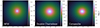 |
Fig. 9. Convergence plots of the primary deflector mass in the composite profile case showing the dark matter profile (left panel), the stellar mass (center panel), and the resulting combined projected mass distribution (right panel). |
In Figure 10, we show the total convergence (left panels) from all mass model components, including explicitly modeled nearby perturbers, for both primary deflector mass model assumptions, power law (top row), and composite (bottom row). For both cases of the underlying mass model, we also include a plot of the magnification model (right panels), which indicates the predicted location of the images for the quadruply and the doubly lensed quasar.
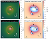 |
Fig. 10. Convergence model (left) and magnification model (right) plots for both mass model assumptions of the primary deflector, the power-law (top), and the composite (bottom) model. The magnification plots indicate the predicted position of the lensed quasar images. |
Figure 11 plots the mean convergence enclosed within a circle of radius r for the dark matter (NFW profile) and baryonic (chameleon profile) components of the composite model and for the power-law model. We find that even under the assumption of a spherical dark matter profile (i.e., omission of ellipticity), the combined convergence of the composite model matches the convergence of the power-law mass profile case in the region where we observe the lensed quasar images. This is further demonstrated in Figure 12, where we show the ratio of the circularized mean convergence between the composite and power-law model main deflector assumption. As illustrated, the resulting convergence of the two model assumptions is nearly identical in the region from around 0.5θE up to approximately 6θE. To differentiate between the two different model parameterization, additional information is required, such as stellar velocity dispersion measurements of the primary deflector’s central region.
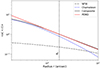 |
Fig. 11. Mean convergence within a circle of radius r. Shown are the components of the composite mass profile assumption for the primary deflector, NFW (black dashdotted line), and chameleon (blue dashed line), along with the combined convergence of the composite case (black solid line) and the power-law profile assumption (red solid line). Also plotted is the effective Einstein radius to provide a reference point. |
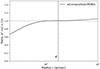 |
Fig. 12. Ratio of the circularized averaged convergence as a function of radius, r, between composite and power-law mass model assumptions of the primary deflector. |
Figure 13 shows models for the reconstructed lensed sources in the source plane for the power-law model profile assumption (top row) and the composite model (bottom row). For each model the reconstructed sources are sorted by band from shortest to longest wavelength, UVIS filters F475X and F814W in the left and center panels, respectively, and IR band F160W in the right panels. The yellow lines in the plots represent the inner and outer caustic lines, corresponding to the critical curves in the image plane, while the position of the sextuply imaged quasar in the source plane is indicated by the blue star.
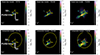 |
Fig. 13. Reconstructed sources for both the power-law and composite models. The yellow lines represent the inner and outer caustics curves of the critical lines. The blue star indicates the location of the sextuply imaged quasar in the source plane. For band F475X, we also mark the positions of the additionally lensed sources, S3 and S4, in the source plane as well as the location of the in-between perturber, S2. |
In Table 3 we list model parameters at the image positions of the sextuply lensed quasar for future microlensing time-delay studies. Specifically, we show total and the stellar convergence at the image positions along with the external shear strength, and the image magnification. The top part of the table tabulates the results of the power-law model assumptions while the lower portion list the composite model results. The stellar convergence for the power-law profile is estimated from reconstructed flux in the F160W (IR) band under the assumption of a constant mass to light ratio. For the composite model assumption, we use the results of the double chameleon profile to estimate the stellar convergence at the image positions.
Lensing results at image positions.
5.2. Model comparisons
The models presented in this paper vary significantly in terms of complexity and underlying assumptions for included model components. Furthermore, during the assessment of systematic uncertainties, we also change the size of the likelihood computation mask used to compute the a model’s χ2 value. To obtain a fair comparison between models, we need to account for the variations in model parameters and number of data points used during the likelihood computation. Therefore, we used BIC, defined in Expression (23), as a proxy to scale the results of each model based on a corresponding statistical weight, w.
Now, the probability of a model Mi given the data, dHST, is formulated as
![Mathematical equation: $$ \begin{aligned} P(M_i | \boldsymbol{d}_{HST} )&\propto P(\boldsymbol{d}_{HST} | M_i) P(M_i) \nonumber \\&\approx {\mathrm{exp}} \left[ -\frac{1}{2} \mathrm{BIC_i} \right] P(M_i). \end{aligned} $$](/articles/aa/full_html/2025/08/aa49984-24/aa49984-24-eq52.gif) (41)
(41)
Hence, the relative probability between two models, M1 and M2, given the data, can be written in terms of the model’s corresponding BIC values:
![Mathematical equation: $$ \begin{aligned} \frac{P(M_1 | \boldsymbol{d}_{HST})}{P(M_2 | \boldsymbol{d}_{HST})} = \mathrm{exp} \left[ -\frac{1}{2} (\mathrm{BIC_1 - BIC_2}) \right]. \end{aligned} $$](/articles/aa/full_html/2025/08/aa49984-24/aa49984-24-eq53.gif) (42)
(42)
We used this formulation of relative probability and followed Birrer et al. (2019) and Shajib et al. (2022) to define the evidence ratio function, f(x), based on the difference between a model’s corresponding BIC value and the lowest BIC among all possible model configurations, BICmin:
![Mathematical equation: $$ \begin{aligned} f(x) \equiv {\left\{ \begin{array}{ll} 1&, x \le {\mathrm{BIC_{min}}}\\ {\mathrm{exp}} \left[ -\frac{1}{2} (x - {\mathrm{BIC_{min}}}) \right]&, x > {\mathrm{BIC_{min}}}. \end{array}\right.} \end{aligned} $$](/articles/aa/full_html/2025/08/aa49984-24/aa49984-24-eq54.gif) (43)
(43)
To find a model’s associated statistical weight, wi, we convolved the evidence ratio with a Gaussian, g, centered on the BIC value for the model with a variance of σBIC2:
 (44)
(44)
The standard deviation, σBIC2, represents the total uncertainty in our models and is composed of statistical fluctuations, σint, and systematic uncertainties, σsys, added in quadrature:
 (45)
(45)
To determine intrinsic fluctuations, σint, that arise from the inherent stochasticity in the MCMC, we run the chain for each model twice. The final statistical scatter added to the total uncertainty in Expression (45) is then computed by averaging the error between the twice executed chains across all models. We assess systematic uncertainties, σsys, in similar fashion as described in Birrer et al. (2019) and Shajib et al. (2022), namely by finding the standard deviation in BIC values between models that differ in terms of configuration or complexity by only one component or only one fixed parameter setting. As with the intrinsic uncertainties, we take the mean of the systematic scatter across all models before adding it to our total error budget, σBIC. Finally, we compute σint to be 20.32 and find σsys = 104.03 for the power-law model and σsys = 240.61 for the composite model, which combine to a total standard deviation for the BIC, used on the computation of the statistical weights (Expression (44)), of σBIC = 106.00 and σBIC = 240.61 for the power-law and composite model, respectively.
Table 4 lists the BIC evaluation for our models sorted from lowest BIC number to highest. Each BIC is computed using the corresponding maximum value of the likelihood sampled in each MCMC chain. Since the radii of the likelihood computation mask differ for the assessment of systematic uncertainties, we separate the modeling results according to the masking radii. We further separate the models based on the mass profile assumption for the primary deflector, power-law versus composite model, and show the difference in BIC for each result with respect to the best fit in each category. For each model we include thecorresponding statistical weight used in the assessment of the total error budget.
BIC evaluations and corresponding statistical weights.
Figure 14 shows the measured image positions in the HST exposures used for our models as well as the astrometric positions of the quasar images as measured by the Gaia satellite. It should be noted that for quasar image F, a Gaia measurement is not available. In Figure 15 we plot the difference in RA and DEC between the measured astrometric image positions of the lensed quasar in our HST exposures and the Gaia astrometric position measurements. To provide reference points for the image position comparison we add a boxes at 10 mas, 40 mas, which corresponds to the pixel size in the UVIS bands. The outer box is drawn at 80 mas, reflecting the size of a pixel in the IR band.
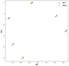 |
Fig. 14. Comparison between HST astrometry image positions and astrometric image positions as measured by the Gaia satellite. |
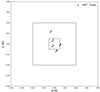 |
Fig. 15. Difference between HST astrometry image positions and astrometric image positions as measured by the Gaia satellite. For reference, boxes are drawn at 10 mas, 40 mas (pixel size in WFC3-UVIS), and 80 mas (drizzled WFC3-IR pixel size). |
As previously indicated, the two assumptions for the main deflector’s mass profile result in a convergence that is nearly identical and differs only in the central region. To demonstrate that it would be possible to distinguish the two models through central stellar velocity dispersion measurements, we show in Figure 16 the line-of-sight velocity dispersion profiles computed for the power-law model (orange line) and for our composite model (blue line). In both cases the dispersion profiles assume a seeing of  and are binned at
  . As demonstrated, we expect the stellar velocity dispersion of the composite model to stay approximately constant within the primary deflector’s center, resulting from the flattened mass profile.
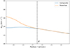 |
Fig. 16. Line-of-sight stellar velocity dispersion profiles for the composite (blue line) and power-law (orange line) assumption of the main deflector mass. Both velocity dispersion profiles assume a |


5.3. Predicted time delays
Assuming a flat ΛCDM cosmology with Ωm = 0.3 we present predictions for measurable time delays between image pairs of the sextuply lensed quasar. Table 5 lists the time delays in days, separated by underlying model assumption for the mass profile of the main deflector, power-law, and composite profile. All delays in Table 5 include a factor of  , where λ represents the MSD factor introduced in Section 2.2, which includes the external convergence, κext, and the internal MST parameter, λint. We define h70 as the dimensionless Hubble constant with value h70 = H0/70 km s−1 Mpc−1.
Predicted time delays between image positions of the sextuply lensed quasar for power-law and composite model assumptions.
We find that the predicted time delays of the composite model agree well with the predictions based on the power-law model assumption. As demonstrated in the plots of Figures 6 and 7, the larger time delays of the imaged quasar are mainly driven by the power-law slope but also show a correlation with the external shear components as well as the Einstein radius of the deflector at redshift z = 1.885.
In Figures 17, 18, 19 we show probability densities of predicted time delays for the image pairs of the sextuply lensed quasar AD, AE, and AF, respectively, based on the models explored during the assessment of systematic uncertainties. We further plot the probability densities for our fiducial power-law model (shown in solid red) and our fiducial model for the composite mass model assumption (shown in solid blue). Combining the probabilities based on the corresponding BIC weight, we also present the aggregate time-delay prediction of the sextuply imaged quasar (solid black line).
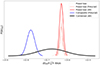 |
Fig. 17. Probability density of predicted time-delay for image pair AD of the sextuply lensed quasar. Shown are the delay predictions for the various power-law models (dotted salmon colored) according to their corresponding BIC weight. Also plotted are the delay predictions for the fiducial power-law model (solid red) and the fiducial composite model (solid blue). The thick black solid line represents the combined probability density of all BIC weighted models. The factor λ represents the presently unknown external convergence and the MST factor, to be determined with ancillary data. |
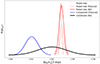 |
Fig. 18. Probability density of predicted time-delay for image pair AE of the sextuply lensed quasar. Shown are the delay predictions for the various power-law models (dotted salmon colored) according to their corresponding BIC weight. Also plotted are the delay predictions for the fiducial power-law model (solid red) and the fiducial composite model (solid blue). The thick black solid line represents the combined probability density of all BIC weighted models. The factor λ represents the presently unknown external convergence and the MST factor, to be determined with ancillary data. |
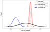 |
Fig. 19. Probability density of predicted time-delay for image pair AF of the sextuply lensed quasar. Shown are the delay predictions for the various power-law models (dotted salmon colored) according to their corresponding BIC weight. Also plotted are the delay predictions for the fiducial power-law model (solid red) and the fiducial composite model (solid blue). The thick black solid line represents the combined probability density of all BIC weighted models. The factor λ represents the presently unknown external convergence and the MST factor, to be determined with ancillary data. |
We do not expect our predicted time delays to agree with those from previous works published before the identification of the Einstein zigzag configuration. However, we performed a comparison in the interest of understanding the history of the modeling of this system. Compared to the time delays presented by Lemon et al. (2022), we find a difference of more than 3 days for the image pair AD and a difference of over 6 days for the quasar pair EF assumed to be doubly imaged by Lemon et al. (2022). The findings presented by Schmidt et al. (2023), showing results of an automated modeling pipeline, have the same difference of slightly over 3 days for the image pair AD. The work in Lemon et al. (2022) and the results in Schmidt et al. (2023) both assume a flat ΛCDM cosmology with H0 = 70 km s−1 Mpc−1.
We can further compare our predicted time delays to the results presented in Mangat et al. (2021). The delay for the doubly lensed quasar in Mangat et al. (2021) is computed to be 88.1 days, using a value for the Hubble constant of H0 = 67.8 km s−1 Mpc−1. Converting this result under the assumption of H0 = 70 km s−1 Mpc−1 and comparing it to the time-delay prediction presented in this paper, we find a difference of more than 12 days. Clearly, these older models should be not be used for any quantitative study.
6. Summary
We have used HST observations of J1721+8842 to reconstruct the mass and light distribution of the system. Utilizing the software package LENSTRONOMY (Birrer & Amara 2018; Birrer et al. 2021), we modeled the multiplane lens system based on two distinct standard assumptions for the parametrization of the main deflector, namely a power-law mass density profile and a composite profile consisting of a dark matter halo and a stellar component that follows the distribution of light. Both underlying parameterization assumptions explicitly describe an Einstein zigzag and reproduce the observed six-image configuration. The main conclusions of our analysis are summarized by the following points:
-
J1721+8842 represents an extraordinary strong lens system comprised of the first-ever discovered sextuply imaged quasar in an Einstein zigzag configuration as the result of strong lensing by two deflectors at different redshifts, which are nearly perfectly aligned with the lensed quasar source along the line of sight. In addition to the multiply imaged quasar and the lensed pertuber located in a higher redshift plane, we found two more lensed galaxies in the source plane, which we included in our models. With these three individually lensed sources and the lensed deflector at redshift z = 1.885, and with resulting images spanning a range of radii, we find that the mass distribution of the primary lensing galaxy is more constrained compared to a typical quad consisting of a single multiply imaged source.
-
Our analysis indicates a correlation between the external shear components and the time delays for image pairs with larger delays (AD, AE, and AF). These longer time delays also correlate with the power-law slope, γ, of the main deflector. Further, we find a dependency for the time delays on the deflector’s mass at redshift z = 1.885. Additionally, the Einstein radius for this “in-between” deflector also exhibits a degeneracy with the nearby perturber P2, in the main deflector plane, as well as with the power-law slope, γ. As our findings indicate, constraining the mass of the nearby perturber P2 could place limits on the mass of the “in-between” pertuber P1 and by extension constrain the predicted time delays even further than the percent level achieved here.
-
In the radial range from approximately 0.5θE to around 6θE, the mean convergence under the central deflector’s best-fit power-law mass profile is nearly identical to that of the composite profile model. In other words, the mass profiles for the two model assumptions (power law versus composite) become effectively indistinguishable in the region where the lensed quasar images are observed.
-
We show that measurements of the central stellar velocity dispersion can be used to differentiate between the underlying model parameterizations. Under the assumption of
 seeing with a circular profile binned at
  , a measurement of the stellar velocity dispersion with a precision of 5–10% interior to
  is sufficient to distinguish the two models.
 -
The time delays for the sextuply imaged quasar, resulting from the first-ever discovered Einstein zigzag configuration, agree at the percent level between both model assumptions for the main deflector (power-law and composite model). In a flat ΛCDM cosmology, with Ωm = 0.3 and ΩΛ = 0.7, the power-law model predicts the following time delays between image pairs, in order from longest to shortest:
 days,
days,  days,
days,  days,
days,  days, and
 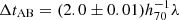 days, with h70 = H0/70 km s−1 Mpc−1 as the dimensionless Hubble constant and λ as the MSD factor, which contains the internal MST parameter, λint, and the external convergence, κext. Using the same cosmology, the time-delay predictions for the combined results of the power-law and composite models, again in order from longest to shortest, are
 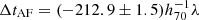 days,
days, 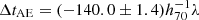 days,
days,  days,
days, 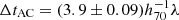 days, and
  days. Even though the analysis for this target was blinded with regard to measured time delays between image pairs, we point out that Dux et al. (2025) find a preliminary delay between images D and E of ΔtDE ∼ −35 days, while the combined result from our power-law and composite models show a delay of
  days for this image pair. Further work is required to combine these measurements to account for the multiplane MSD, as discussed below.
A future paper will build on our models and time-delay predictions for J1721+8842 and incorporate measurements of observed time delay, a spectroscopic measurement of the stellar velocity dispersion, and an estimate for the external convergence based on a model for the line-of-sight mass distribution to present a complete H0 inference. Furthermore, the unusual configuration means that we have to consider the possibility of a mass sheet and external shear within both the main-deflector plane and the redshift z = 1.885 plane. Considering the degeneracy between the mass of the in-between deflector P1 and the observed time delays, constraining the mass sheet and shear in the z = 1.885 plane will be crucial for cosmological analysis. At the same time, the unique configuration gives us some leverage in addressing this degeneracy with lensing data alone. These topics will be addressed in a future paper (Millon et al., in prep.).
Acknowledgments
This research is based on observations made with the NASA/ESA Hubble Space Telescope obtained from the Space Telescope Science Institute, which is operated by the Association of Universities for Research in Astronomy, Inc., under NASA contract NAS 5-26555. These observations are associated with programs HST-GO-15320 and HST-GO-15652. Support for the two programs was provided by NASA through a grant from the Space Telescope Science Institute, which is operated by the Association of Universities for Research in Astronomy, Inc., under NASA contract NAS 5-26555. We thank the referee for constructive reports. TS TT acknowledge support by the National Science Foundation through grant NSF-AST-1906976 and NSF-AST-1907396 “Collaborative Research: Toward a 1% measurement of the Hubble Constant with gravitational time delays”. TT acknowledges support by the Gordon and Betty Moore Foundation. MM acknowledges support by the Swiss National Science Foundation (SNSF) through mobility grant P500PT_203114. SB acknowledges support from the Department of Physics & Astronomy, Stony Brook University. DS acknowledges the support of the Fonds de la Recherche Scientifique-FNRS, Belgium, under grant No. 4.4503.1. This work is also supported by NASA through the NASA Hubble Fellowship grant HST-HF2-51492 awarded to AJS by the Space Telescope Science Institute, which is operated by the Association of Universities for Research in Astronomy, Inc., for NASA, under contract NAS5-26555. AJS also received support from NASA through the Space Telescope Science Institute grants HST-GO-16773 and JWST-GO-2974. AG FC acknowledge funding and support by the SNSF. This project has received funding from the European Union’s Horizon Europe research and innovation programme under the Marie Sklodovska-Curie grant agreement No 101105725. This work has received support by the Swiss National Science Foundation (SNSF) and by the European Research Council (ERC) under the European Unions Horizon 2020 research and innovation programme (COSMICLENS: grant agreement No 787886). This research made use of LENSTRONOMY (Birrer & Amara 2018; Birrer et al. 2021), EMCEE (Foreman-Mackey et al. 2013), FASTELL (Barkana 1998), SEXTRACTOR (Bertin & Arnouts 1996), NUMPY (Oliphant 2015), SCIPY (Jones et al. 2001), ASTROPY (Astropy Collaboration 2018), JUPYTER (Kluyver et al. 2016), MATPLOTLIB (Hunter 2007), SEABORN (Waskom 2021), GETDIST (https://github.com/cmbant/getdist), and STARRED (Michalewicz et al. 2023; Millon et al. 2024).
References
- Abdalla, E., Abellán, G. F., Aboubrahim, A., et al. 2022, J. High Energy Astrophys., 34, 49 [NASA ADS] [CrossRef] [Google Scholar]
- Astropy Collaboration (Price-Whelan, A. M., et al.) 2018, AJ, 156, 123 [Google Scholar]
- Avila, R. J., Hack, W., Cara, M., et al. 2015, in Astronomical Data Analysis Software an Systems XXIV (ADASS XXIV), eds. A. R. Taylor, & E. Rosolowsky, Astronomical Society of the Pacific Conference Series, 495, 281 [NASA ADS] [Google Scholar]
- Barkana, R. 1998, ApJ, 502, 531 [NASA ADS] [CrossRef] [Google Scholar]
- Bertin, E., & Arnouts, S. 1996, A&AS, 117, 393 [NASA ADS] [CrossRef] [EDP Sciences] [Google Scholar]
- Birrer, S., & Amara, A. 2018, Phys. Dark Universe, 22, 189 [NASA ADS] [CrossRef] [Google Scholar]
- Birrer, S., Amara, A., & Refregier, A. 2015, ApJ, 813, 102 [Google Scholar]
- Birrer, S., Amara, A., & Refregier, A. 2016, JCAP, 2016, 020 [CrossRef] [Google Scholar]
- Birrer, S., Treu, T., Rusu, C. E., et al. 2019, MNRAS, 484, 4726 [Google Scholar]
- Birrer, S., Shajib, A., Gilman, D., et al. 2021, J. Open Source Softw., 6, 3283 [NASA ADS] [CrossRef] [Google Scholar]
- Birrer, S., Millon, M., Sluse, D., et al. 2024, Space Sci. Rev., 220, 48 [NASA ADS] [CrossRef] [Google Scholar]
- Blandford, R. D., & Narayan, R. 1992, ARA&A, 30, 311 [NASA ADS] [CrossRef] [Google Scholar]
- Bolton, A. S., Burles, S., Koopmans, L. V. E., Treu, T., & Moustakas, L. A. 2006, ApJ, 638, 703 [NASA ADS] [CrossRef] [Google Scholar]
- Bonvin, V., Courbin, F., Suyu, S. H., et al. 2017, MNRAS, 465, 4914 [NASA ADS] [CrossRef] [Google Scholar]
- Chen, G. C. F., Fassnacht, C. D., Suyu, S. H., et al. 2022, MNRAS, 513, 2349 [NASA ADS] [CrossRef] [Google Scholar]
- Collett, T. E., & Bacon, D. J. 2016, MNRAS, 456, 2210 [CrossRef] [Google Scholar]
- Di Valentino, E., Mena, O., Pan, S., et al. 2021, Class. Quant. Grav., 38, 153001 [NASA ADS] [CrossRef] [Google Scholar]
- Dutton, A. A., Brewer, B. J., Marshall, P. J., et al. 2011, MNRAS, 417, 1621 [NASA ADS] [CrossRef] [Google Scholar]
- Dux, F., Millon, M., Lemon, C., et al. 2025, A&A, 694, A300 [NASA ADS] [CrossRef] [EDP Sciences] [Google Scholar]
- Eisenstein, D. J., Zehavi, I., Hogg, D. W., et al. 2005, ApJ, 633, 560 [Google Scholar]
- Ertl, S., Schuldt, S., Suyu, S. H., et al. 2023, A&A, 672, A2 [NASA ADS] [CrossRef] [EDP Sciences] [Google Scholar]
- Faber, S. M., & Jackson, R. E. 1976, ApJ, 204, 668 [Google Scholar]
- Falco, E. E., Gorenstein, M. V., & Shapiro, I. I. 1985, ApJ, 289, L1 [Google Scholar]
- Foreman-Mackey, D., Hogg, D. W., Lang, D., & Goodman, J. 2013, PASP, 125, 306 [Google Scholar]
- Gavazzi, R., Treu, T., Rhodes, J. D., et al. 2007, ApJ, 667, 176 [Google Scholar]
- Golse, G., & Kneib, J.-P. 2002, A&A, 390, 821 [NASA ADS] [CrossRef] [EDP Sciences] [Google Scholar]
- Hunter, J. D. 2007, Comput. Sci. Eng., 9, 90 [NASA ADS] [CrossRef] [Google Scholar]
- Jones, E., Oliphant, T., Peterson, P., et al. 2001, SciPy: Open source scientific tools for Python, http://www.scipy.org/ [Google Scholar]
- Kluyver, T., Ragan-Kelley, B., Pérez, F., et al. 2016, in Positioning and Power in Academic Publishing: Players, Agents and Agendas, eds. F. Loizides, & B. Schmidt (Amsterdam, Netherlands: IOS Press BV), 87 [Google Scholar]
- Knox, L., & Millea, M. 2020, Phys. Rev. D, 101, 043533 [Google Scholar]
- Lemon, C. A., Auger, M. W., McMahon, R. G., & Ostrovski, F. 2018, MNRAS, 479, 5060 [Google Scholar]
- Lemon, C., Millon, M., Sluse, D., et al. 2022, A&A, 657, A113 [NASA ADS] [CrossRef] [EDP Sciences] [Google Scholar]
- Mangat, C. S., McKean, J. P., Brilenkov, R., et al. 2021, MNRAS, 508, L64 [NASA ADS] [CrossRef] [Google Scholar]
- McCully, C., Keeton, C. R., Wong, K. C., & Zabludoff, A. I. 2017, ApJ, 836, 141 [NASA ADS] [CrossRef] [Google Scholar]
- Michalewicz, K., Millon, M., Dux, F., & Courbin, F. 2023, J. Open Source Softw., 8, 5340 [NASA ADS] [CrossRef] [Google Scholar]
- Millon, M., Michalewicz, K., Dux, F., Courbin, F., & Marshall, P. J. 2024, AJ, 168, 55 [NASA ADS] [CrossRef] [Google Scholar]
- Navarro, J. F., Frenk, C. S., & White, S. D. M. 1997, ApJ, 490, 493 [Google Scholar]
- Oliphant, T. E. 2015, Guide to NumPy, 2nd edn. (USA: CreateSpace Independent Publishing Platform) [Google Scholar]
- Perlmutter, S., Aldering, G., Goldhaber, G., et al. 1999, ApJ, 517, 565 [Google Scholar]
- Planck Collaboration VI. 2020, A&A, 641, A6 [NASA ADS] [CrossRef] [EDP Sciences] [Google Scholar]
- Refregier, A. 2003, MNRAS, 338, 35 [Google Scholar]
- Refsdal, S. 1964, MNRAS, 128, 307 [NASA ADS] [CrossRef] [Google Scholar]
- Riess, A. G., Filippenko, A. V., Challis, P., et al. 1998, AJ, 116, 1009 [Google Scholar]
- Riess, A. G., Yuan, W., Macri, L. M., et al. 2022, ApJ, 934, L7 [NASA ADS] [CrossRef] [Google Scholar]
- Saha, P. 2000, AJ, 120, 1654 [Google Scholar]
- Saha, P., Coles, J., Macciò, A. V., & Williams, L. L. R. 2006, ApJ, 650, L17 [NASA ADS] [CrossRef] [Google Scholar]
- Schmidt, T., Treu, T., Birrer, S., et al. 2023, MNRAS, 518, 1260 [Google Scholar]
- Schneider, P. 2019, A&A, 624, A54 [NASA ADS] [CrossRef] [EDP Sciences] [Google Scholar]
- Schneider, P., & Sluse, D. 2014, A&A, 564, A103 [NASA ADS] [CrossRef] [EDP Sciences] [Google Scholar]
- Schneider, P., Ehlers, J., & Falco, E. E. 1992, Gravitational Lenses, XIV (Springer-Verlag Berlin Heidelberg New York), 560 [Google Scholar]
- Schöneberg, N., Abellán, G. F., Sánchez, A. P., et al. 2022, Phys. Rep., 984, 1 [CrossRef] [Google Scholar]
- Sérsic, J. L. 1968, Atlas de Galaxias Australes (Cordoba, Argentina: Observatorio Astronomico) [Google Scholar]
- Shajib, A. J., Birrer, S., Treu, T., et al. 2019, MNRAS, 483, 5649 [Google Scholar]
- Shajib, A. J., Birrer, S., Treu, T., et al. 2020, MNRAS, 494, 6072 [Google Scholar]
- Shajib, A. J., Wong, K. C., Birrer, S., et al. 2022, A&A, 667, A123 [NASA ADS] [CrossRef] [EDP Sciences] [Google Scholar]
- Sluse, D., Sonnenfeld, A., Rumbaugh, N., et al. 2017, MNRAS, 470, 4838 [NASA ADS] [CrossRef] [Google Scholar]
- Suyu, S. H., Marshall, P. J., Auger, M. W., et al. 2010, ApJ, 711, 201 [Google Scholar]
- Suyu, S. H., Treu, T., Hilbert, S., et al. 2014, ApJ, 788, L35 [NASA ADS] [CrossRef] [Google Scholar]
- Treu, T., & Koopmans, L. V. E. 2002, ApJ, 575, 87 [NASA ADS] [CrossRef] [Google Scholar]
- Treu, T., & Marshall, P. J. 2016, A&ARv, 24, 11 [Google Scholar]
- Treu, T., & Shajib, A. J. 2024, in The Hubble Constant Tension, eds. E. Di Valentino, & B. Dillon, 251 [Google Scholar]
- Treu, T., Suyu, S. H., & Marshall, P. J. 2022, A&ARv, 30, 8 [NASA ADS] [CrossRef] [Google Scholar]
- Vagnozzi, S. 2023, Universe, 9, 393 [NASA ADS] [CrossRef] [Google Scholar]
- Waskom, M. 2021, J. Open Source Softw., 6, 3021 [CrossRef] [Google Scholar]
All Tables
Flexion shift estimates for nearby perturbers based on a corresponding flux ratio analysis.
Predicted time delays between image positions of the sextuply lensed quasar for power-law and composite model assumptions.
All Figures
|
Fig. 1. Red-green-blue composite image of J1721+8842 and nearby perturbers created by exposures in the HST band F160W (red), F814W (blue), and F475X (green). |
| In the text | |
|
Fig. 2. Red-green-blue composite image of J1721+8842 created by exposures in the HST band F160W (red), F814W (blue), and F475X (green). |
| In the text | |
|
Fig. 3. Priors on Einstein radii for nearby perturbing galaxies explicitly included in the models. |
| In the text | |
|
Fig. 4. Reconstructed power-law model for J1721+8842. The first column (left) shows the observations in each band, sorted by wavelength from short to long. The second column (center) displays the reconstructed model for each filter, and in the third column (right) are the normalized residuals between our model and the observed data. |
| In the text | |
|
Fig. 5. Reconstructed composite model for J1721+8842. The first column (left) shows the observations in each band, sorted by wavelength from short to long. The second column (center) displays the reconstructed model for each filter, and in the third column (right) are the normalized residuals between our model and the observed data. |
| In the text | |
|
Fig. 6. Mass model parameters and predicted time delays for the two underlying assumptions of the primary deflector’s mass profile. The power-law model results are shown in red while the results for the composite model are colored in blue. In the composite model case, the Einstein radius of the main deflector, P0, is calculated via the circularized average of the convergence and the power-law slope represents the derivative of the convergence at the Einstein radius. To address computational challenges in sampling the composite model parameter space, the external shear is held fixed at the power-law model results, and therefore no composite model posteriors are shown. |
| In the text | |
|
Fig. 7. Power-law slope, Einstein radii for both deflectors, P0 (main deflector) and P1, and predicted time delays for the two mass profile assumptions of the main deflector. The power-law and composite model results are shown in colors red and blue, respectively. In the composite model case, the Einstein radius of the main deflector, P0, is calculated via the circularized average of the convergence and the power-law slope represents the derivative of the convergence at the Einstein radius. To address computational challenges in sampling the composite model parameter space, the mass of deflector P1 is held fixed at the power-law model results, and therefore no composite model posteriors are shown. |
| In the text | |
|
Fig. 8. Comparison of the main deflector and the perturber Einstein raddii for the power-law mass model assumption. |
| In the text | |
|
Fig. 9. Convergence plots of the primary deflector mass in the composite profile case showing the dark matter profile (left panel), the stellar mass (center panel), and the resulting combined projected mass distribution (right panel). |
| In the text | |
|
Fig. 10. Convergence model (left) and magnification model (right) plots for both mass model assumptions of the primary deflector, the power-law (top), and the composite (bottom) model. The magnification plots indicate the predicted position of the lensed quasar images. |
| In the text | |
|
Fig. 11. Mean convergence within a circle of radius r. Shown are the components of the composite mass profile assumption for the primary deflector, NFW (black dashdotted line), and chameleon (blue dashed line), along with the combined convergence of the composite case (black solid line) and the power-law profile assumption (red solid line). Also plotted is the effective Einstein radius to provide a reference point. |
| In the text | |
|
Fig. 12. Ratio of the circularized averaged convergence as a function of radius, r, between composite and power-law mass model assumptions of the primary deflector. |
| In the text | |
|
Fig. 13. Reconstructed sources for both the power-law and composite models. The yellow lines represent the inner and outer caustics curves of the critical lines. The blue star indicates the location of the sextuply imaged quasar in the source plane. For band F475X, we also mark the positions of the additionally lensed sources, S3 and S4, in the source plane as well as the location of the in-between perturber, S2. |
| In the text | |
|
Fig. 14. Comparison between HST astrometry image positions and astrometric image positions as measured by the Gaia satellite. |
| In the text | |
|
Fig. 15. Difference between HST astrometry image positions and astrometric image positions as measured by the Gaia satellite. For reference, boxes are drawn at 10 mas, 40 mas (pixel size in WFC3-UVIS), and 80 mas (drizzled WFC3-IR pixel size). |
| In the text | |
|
Fig. 16. Line-of-sight stellar velocity dispersion profiles for the composite (blue line) and power-law (orange line) assumption of the main deflector mass. Both velocity dispersion profiles assume a |
| In the text | |
|
Fig. 17. Probability density of predicted time-delay for image pair AD of the sextuply lensed quasar. Shown are the delay predictions for the various power-law models (dotted salmon colored) according to their corresponding BIC weight. Also plotted are the delay predictions for the fiducial power-law model (solid red) and the fiducial composite model (solid blue). The thick black solid line represents the combined probability density of all BIC weighted models. The factor λ represents the presently unknown external convergence and the MST factor, to be determined with ancillary data. |
| In the text | |
|
Fig. 18. Probability density of predicted time-delay for image pair AE of the sextuply lensed quasar. Shown are the delay predictions for the various power-law models (dotted salmon colored) according to their corresponding BIC weight. Also plotted are the delay predictions for the fiducial power-law model (solid red) and the fiducial composite model (solid blue). The thick black solid line represents the combined probability density of all BIC weighted models. The factor λ represents the presently unknown external convergence and the MST factor, to be determined with ancillary data. |
| In the text | |
|
Fig. 19. Probability density of predicted time-delay for image pair AF of the sextuply lensed quasar. Shown are the delay predictions for the various power-law models (dotted salmon colored) according to their corresponding BIC weight. Also plotted are the delay predictions for the fiducial power-law model (solid red) and the fiducial composite model (solid blue). The thick black solid line represents the combined probability density of all BIC weighted models. The factor λ represents the presently unknown external convergence and the MST factor, to be determined with ancillary data. |
| In the text | |
Current usage metrics show cumulative count of Article Views (full-text article views including HTML views, PDF and ePub downloads, according to the available data) and Abstracts Views on Vision4Press platform.
Data correspond to usage on the plateform after 2015. The current usage metrics is available 48-96 hours after online publication and is updated daily on week days.
Initial download of the metrics may take a while.