| Issue |
A&A
Volume 700, August 2025
|
|
|---|---|---|
| Article Number | A51 | |
| Number of page(s) | 7 | |
| Section | The Sun and the Heliosphere | |
| DOI | https://doi.org/10.1051/0004-6361/202450220 | |
| Published online | 04 August 2025 | |
Formation of magnetic switchbacks via expanding Alfvén waves
1
Space Sciences Laboratory, University of California, 7 Gauss Way, Berkeley, CA 94720, USA
2
Physics Department, University of California, Berkeley, CA 94720, USA
3
Department of Physics, University of Otago, 730 Cumberland St., Dunedin 9016, New Zealand
4
Department of Physics & Astronomy, University of New Hampshire, Durham, NH 03824, USA
5
LPC2E, CNRS and University of Orléans, Orléans, France
6
ISSI, Bern, Switzerland
7
Harvard & Smithsonian Center for Astrophysics, Cambridge, MA, USA
⋆ Corresponding author: This email address is being protected from spambots. You need JavaScript enabled to view it.
Received:
2
April
2024
Accepted:
21
May
2025
Abstract
Context. Large-amplitude inversions of the solar wind’s interplanetary magnetic field have long been documented; however, observations from the Parker Solar Probe (PSP) mission have renewed interest in this phenomenon as such features, often termed switchbacks, may constrain both the sources of the solar wind as well as in situ nonlinear dynamics and turbulent heating.
Aims. We aim to show that magnetic field fluctuations in the solar wind are consistent with Alfvénic fluctuations that naturally form switchback inversions in the magnetic field through expansion effects.
Methods. We examine PSP observations of the evolution of a single stream of solar wind in a radial scan from PSP’s tenth perihelion encounter from ≈15 − 50 R⊙. We study the growth and radial scaling of normalized fluctuation amplitudes in the magnetic field, δB/B, within the framework of spherical polarization. We compare heating rates computed via outer-scale decay from consideration of wave action to proton heating rates empirically observed through adiabatic expansion.
Results. We find that the magnetic field fluctuations are largely spherically polarized and that the normalized amplitude of the magnetic field, δB/B, increases with amplitude. The growth of the magnetic field amplitude leads to switchback inversions in the magnetic field. While the amplitude does not grow as fast as is predicted by the conservation of wave action, the deviation from the expected scaling yields an effective heating rate that is close to the empirically observed proton heating rate.
Conclusions. The observed scaling of fluctuation amplitudes is largely consistent with a picture of expanding Alfvén waves that seed turbulence, leading to dissipation. The expansion of the waves leads to the growth of wave amplitudes, resulting in the formation of switchbacks.
Key words: Sun: atmosphere / Sun: heliosphere / Sun: magnetic fields / solar wind
© The Authors 2025
 Open Access article, published by EDP Sciences, under the terms of the Creative Commons Attribution License (https://creativecommons.org/licenses/by/4.0), which permits unrestricted use, distribution, and reproduction in any medium, provided the original work is properly cited.
This article is published in open access under the Subscribe to Open model. This email address is being protected from spambots. You need JavaScript enabled to view it. to support open access publication.
1. Introduction
Fluctuations in the solar wind at scales much larger than ion-kinetic scales are often approximated in the framework of magnetohydrodynamics (MHD), which provides a complete description of the spatiotemporal evolution of the magnetic field, plasma flow velocity, and plasma density. Linearization of the MHD equations in terms of small-amplitude plane waves identifies eigenmodes corresponding both to propagating waves and non-propagating structures that share characteristics with observed solar wind fluctuations. The Alfvén (1942) mode, which is associated with proportional magnetic field and velocity fluctuations, δv ∝ δB, is known to agree well with observed polarization signatures of the solar wind (Belcher & Davis 1971).
While small amplitude approximations to MHD are useful in describing observed turbulence, the solar wind is often subject to large-amplitude fluctuations in the magnetic field with (|δb|/|b0|∼1) that maintain a constant magnitude,

and appear to be spherically polarized (Goldstein et al. 1974; Lichtenstein & Sonett 1980; Riley et al. 1996; Gosling et al. 2009). Constant magnitude fluctuations are highly prevalent in the inner heliosphere observed by PSP (Dudok de Wit et al. 2020; Dunn et al. 2023). These fluctuations share characteristics of finite- and large-amplitude Alfvén waves, which maintain the constant magnitude of the total magnetic field (Barnes & Hollweg 1974; Goldstein et al. 1974), and thus appear spherically or arc-polarized. Specifically, large-amplitude fluctuations in the solar wind have a component parallel, the mean field, which maintains Alfvénic correlations (Matteini et al. 2015); consequently, these fluctuations appear as “one-sided” enhancements in the solar wind velocity (Gosling et al. 2009; Matteini et al. 2015). The constraints imposed by the large-amplitude nature contrast with the small-amplitude Alfvén mode, which is a fluctuation purely perpendicular to the mean magnetic field. The large-amplitude arc and spherically polarized Alfvén modes are, like the small-amplitude (linear, plane-polarized) Alfvén mode, exact solutions of MHD, and thus their ability to dissipate energy at large scales is negligible. Accordingly, even in these large-amplitude states, which have recently been shown to occur in hybrid-kinetic models (Matteini et al. 2024), a turbulent cascade or other nonlinearities (Tenerani et al. 2020) must drive energy in the large amplitude fluctuations to smaller, dissipative scales.
Recent observations from NASA’s Parker Solar Probe (PSP) mission highlight large-amplitude inversions of the magnetic field, (Bale et al. 2019; Kasper et al. 2019; Dudok de Wit et al. 2020) many of which are strongly Alfvénic (Horbury et al. 2020; Laker et al. 2021; Mozer et al. 2020; Larosa et al. 2021). These fluctuations, which have been termed “switchbacks” (SBs), are a signature of solar wind sources, and may be important in the energy budget of the solar wind heating as it expands into the heliosphere. The origin of large-amplitude SB fluctuations is a subject of significant debate and a comprehensive discussion is found in Raouafi et al. (2023a). In this paper, we focus on the connection between spherically polarized waves and the in situ development of SBs.
Several authors have suggested that SBs likely arise in the in situ growth of Alfvén waves in an expanding solar wind (Shoda et al. 2021; Squire et al. 2020; Mallet et al. 2021; Johnston et al. 2022), which explicitly couples the SB fluctuations to the large-amplitude Alfvénic state. Here, we perform an observational analysis of the radial evolution of the spherically polarized, constant magnitude state. We identify a stream of fast wind in which the magnetic field fluctuations maintain strong spherical polarization as they propagate outward; a stationary frame of the observed fluctuations is identified using de Hoffmann-Teller (dHT) analysis and found to approximate the Alfvén speed well, suggesting that these spherically polarized waves are indeed Alfvén waves. Bowen et al. (2025) have performed an analysis of the nonlinear turbulent interactions that occur in these states. The application of conservation of wave-action (Heinemann & Olbert 1980; Chandran & Hollweg 2009) demonstrates that the evolution of fluctuations in the stream is consistent with Wentzel–Kramers–Brillouin (WKB) expansion of large amplitude waves undergoing some amount of turbulent dissipation, which we find is consistent with proton heating rates. Expansion leads to the growth of the normalized fluctuation amplitude, dB/B, where dB is understood as the root mean square (RMS) amplitude of δB, leading to larger rotations in the field that resemble SBs. The growth of dB/B leads to larger fractions of the solar wind magnetic field “switching back” at larger distances. These results suggest that SBs form in situ in the solar wind and that the decay of the large-amplitude state is a dominant contributor to solar wind heating.
2. Parker Solar Probe observations
We studied a five-day stream from PSP’s tenth perihelion encounter from November 16 to 21, 2021. During this interval, PSP traversed from a heliocentric distance of 54.9R⊙ down to 14.3 R⊙. The Encounter 10 stream is thought to be connected to a single coronal hole (Badman et al. 2023) and the dynamical outer-scale evolution has previously been studied by Davis et al. (2023) and Huang et al. (2023), who report the growth of turbulence from an outer-scale population of Alfvénic fluctuations. Magnetic field data were obtained from the electromagnetic PSP/FIELDS experiment Bale et al. (2016) and proton moments from the PSP/SWEAP investigation’s (Kasper et al. 2016) electrostatic analyzer (Livi et al. 2022).
We separated the interval into N = 355 one hour sub-intervals. Each sub-interval overlaps its neighbors by two thirds; that is, each sub-interval starts 20 minutes after the start of the previous sub-interval. Overlapping was used to increase statistics. In each sub-interval we computed the mean magnetic field vector, B0 = ⟨B⟩, and its magnitude, B0 = |B0|. We also computed the mean magnetic field magnitude, B = ⟨|B|⟩, the mean solar wind speed, Vsw = |⟨Vp⟩|, and the Alfvén speed,  , where μ0 is the magnetic permeability and ρ0 is the mean mass density of each hour computed from quasithermal noise densities (Moncuquet et al. 2020; Pulupa et al. 2017). We defined η = (VA/Vsw)2 following Chandran & Hollweg (2009).
Figure 1(a-c) show the vector magnetic field, the normalized BR/|B| component, and the solar wind velocity vector of the interval, respectively, as a function of the radial distance, R. Figure 1(d) shows estimates of η, VA, and Vsw computed in each sub-interval, along with the power-law fits to each quantity in the form  .
.
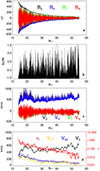 |
Fig. 1. a) FIELDS magnetic field data in RTN coordinates. The magnitude, |B|, is shown in black. b) Radial component of magnetic field normalized to field magnitude BR/|B|. Large-scale inversions in BR known as SBs are observed. c) SWEAP SPAN velocity measurements in RTN coordinates. |V| is shown in black. d) Computed dHT frame speed, VdHT, Alfvén speed, VA, and average wind speed, Vsw, and η = (VA/Vsw)2. |
Figure 1(d) additionally shows the de Hoffmann Teller (dHT) frame computed in each hour-long interval. The dHT frame minimizes the RMS value of the convected electric field, E = −v × B (Khrabrov & Sonnerup 1998), corresponding to aligned magnetic and velocity fluctuations. The frame with zero electric field corresponds to a stationary frame for electromagnetic fluctuations with no parallel electric field, such as Alfvén waves. We obtained the dHT by minimizing E2 for each interval:
 (1)
(1)
 (2)
(2)
The dHT frame, VdHT, is invariant under multiplicative scalings of B, and is thus not sensitive to Alfvénic normalization. Matteini et al. (2015) previously used the dHT frame to study the minimization of the convected electric field via spherical polarization. Additionally, the dHT has been used to study and classify SBs (Horbury et al. 2020). Recently, Agapitov et al. (2023) demonstrated that a shared dHT exists between the SB fluctuations and the surrounding solar wind. Figure 1(d) shows that the magnitude of the dHT frame, |VdHT|, follows the Alfvén speed closely, which suggests that the outer, 1 hour long scales consist predominantly of Alfvénic fluctuations.
In each interval we also computed the RMS fluctuation quantity of the magnetic field, dB; we furthermore computed RMS quantities of the magnetic field perpendicular to the mean field, dB⊥, and parallel to the mean field, dB∥. To highlight the spherically polarized nature of this stream, we fit the vector magnetic field data in each sub-interval to a spherical shell of constant magnetic field magnitude, Bsph, using linear least square optimization techniques. We projected each vector magnetic field measurement onto the spherical shell to produce a spherically polarized Bsph, which points parallel to the measured B at each time, but with a constant magnitude, |Bsph|. We computed the RMS fluctuation quantities of the spherically polarized magnetic field perpendicular to the mean field,  , parallel to the mean field
  . Furthermore, we computed the residuals, BC = B − Bsph, corresponding to compressible fluctuations off the spherical shell, and report their average values for each interval as
  . As the spherically polarized Bsph vector is parallel to Bsph at each measurement, the deviation off the sphere is essentially equal to |B|−⟨|B|⟩, such that dBC is equivalent to the RMS of d|B|.
Figure 2(a) shows the radial dependence of RMS quantities dB⊥, dB∥, while Figure 2(b) shows the spherically confined quantities  ,
,  alongside dBC and B0. The spherically constrained
  ,
,  are nearly identical to the unconstrained quantities, indicating the strong spherical polarization throughout the stream. The deviation from the sphere is dBC, and significantly smaller than the perpendicular or parallel RMS fluctuations, indicating that the data in each interval is well fit by a sphere.
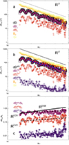 |
Fig. 2. a) Root mean squared dB, dB⊥, and dB∥ (black, maroon, red); magnitude of the mean magnetic field, B0, orange. b) Spherically confined fluctuations, dB, dB⊥, and dB∥, (black, maroon, red) where all fluctuations maintain a constant magnitude, |Bsph|. The RMS residual fluctuations between the total field and spherically polarized field, dBC, are shown in dark blue. The dashed red line shows the wave amplitude from conservation of wave action with no dissipation. The blue line shows the best fit to dBsph. c) Normalized amplitudes, dB⊥sph/B0, dB∥sph/B0, and |

Given the strong spherical polarization, which includes significant fluctuations parallel to the mean and which maintains a stationary dHT frame that is consistent with the Alfvén speed, we argue that the spherically polarized magnetic field fluctuations correspond to an outward propagating, finite-amplitude Elsasser mode, z± = v ± b with z+ ≈ 2bsph, where  . We used a linear least square fit in log-log space of dBsph and radius, R/R⊙, to approximate power-law scalings,
  ; we find that αdB = 1.67, which is shown in blue in Figure 2(b).
The quantity η was used to define the quantities, g±, from the Elsasser fluctuations, z±, as
 (3)
(3)
The quantity g+2, which corresponds to the outward-propagating Elsasser variable z+, is ideally conserved in the absence of dissipation and heating, and is conserved even for large-amplitude fluctuations, so long as they remain spherically polarized Hollweg (1974). We computed dz+ = 2dBsph/μ0ρ from a linear least square fit in log space of the form  . Using dz0+, we defined dg0+. We computed dissipationless scalings for
  and
and  from Equation (3), g0+, and the scaling of
  ; the dissipationless dB′(R), with the approximate power law scaling αdB′ = 1.22, was similarly computed and is plotted in red in Figure 2(b).
Figure 2(c) shows normalized amplitudes, dB/B0, which grow with the radius. We computed a power law fit to dB⊥sph/B0 with a scaling of R0.31. The dissipationless scaling of dBsph′/B0, which is how the amplitudes would grow without heating, is found to be R0.68. We computed a power law fit to dB∥sph/B0 with a scaling of R0.41. Compressible fluctuations, dBC/B0, remain at ≈0.01 of the mean magnetic field up until about 50R⊙, when there is significant growth.
The observed deviation of dB from the dissipationless dB′(R) indicates the decay of large-amplitude fluctuations, likely associated with dissipation and extended heating of the solar wind. Following Chandran & Hollweg (2009) and Chandran & Perez (2019), we obtained a decay rate for the large-scale Alfvénic fluctuations as
 (4)
(4)
where the derivative,  , was obtained from the power-law fit,
  . Importantly, this estimate of Q(R) in Eq. (4) should correspond to the total turbulent heating rate that is deposited in both ions and electrons.
Figure 3(a) shows the estimated heating rate from the conservation of wave action, Q(R). We compared this quantity to the proton and electron heating rates, Qe, p, as well as the turbulent cascade rate, ϵ. Recent work has highlighted that an analysis of the proton heating rate is best obtained via a direct analysis of particle properties (Zaslavsky 2023; Mozer et al. 2023). For each individual sample in the stream we computed the pressure perpendicular and parallel to the magnetic field, p⊥ and p∥, and the constants, C∥ = p∥B2/n3 and C⊥ = p⊥/nB, which are related to the heating terms, Qp⊥ and Qp∥, via
 (5)
(5)
 (6)
(6)
(Chew et al. 1956; Zaslavsky 2023; Mozer et al. 2023). The anisotropic pressures were computed from the PSP SPAN-I Temperature tensor (Livi et al. 2022), which was rotated into field-aligned coordinates (FACs). We included only SPAN-I observations for which more than 60 energy bins had finite, non-zero counts, which was intended to remove observations for which the plasma is out of SPAN’s limited field of view. We additionally implemented drifting bi-Maxwellian fits of a core and beam population to the SPAN-i data (Bowen et al. 2024b) and computed effective parallel and perpendicular pressures following Klein et al. (2021); no significant deviations were found when implementing the moments versus the fit approximations to the SPAN-i data.
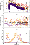 |
Fig. 3. a) Radial scaling of dissipation rates computed from WKB expansion of outer scale fluctuations, Q (black), from Chandran et al. (2009), CGL estimate of proton heating, Qp (yellow), following Zaslavsky (2023), third-order cascade rate, ϵ (Politano & Pouquet 1998), and electron heating, Qe (Cranmer et al. 2009). Solid lines show the moving-window median value. b) Ratios of dissipation quantities, ϵ/Q (red), Qp/Q (yellow), Qp⊥/Qp (black), and Qp∥/Qp (purple). c) PDFs of ratios Qp/Q (yellow), ϵ/Q (red), ϵ/Qp (orange), and Qp/Qe (purple). |
We computed power-law fits,  and
and  , from which Qp was estimated as
 (7)
(7)
and the time derivative was approximated using the convective derivative, d/dt = Vswd/dR. Figure 3(a) shows Qp = Qp⊥ + Qp∥ to demonstrate a general agreement between the total proton heating observed from the plasma parameters and the expected heating from the deviations from conservation of wave action in Equation (4). There is some subtlety to the use of |B| or B0 in the Chew et al. (1956) approach (Marsch et al. 1983; Perrone et al. 2019; Zaslavsky 2023); though we leave in-depth discussion to conserved and invariant quantities to future discussion, we do note that the use of |B| or B0 in Equation (7) results in only a 10% difference in heating rates.
We additionally considered the electron heating through scaling of the QTN estimate of the electron temperature, Moncuquet et al. (2020) which is available up to approximately 40R⊙. Though we do not have measurements of electron temperature anisotropy to perform the CGL analysis, we implemented the following electron heating formula:
 (8)
(8)
(Cranmer et al. 2009; Bandyopadhyay et al. 2023), where terms corresponding to collisional heating and the Parker spiral effects are omitted due to their minimal effects. We have also omitted consideration of the heat flux, which is likely negligible compared to contributions from wave heating Halekas et al. (2023) in these faster streams. Though heat flux is likely important for the electron energy budget in the inner heliosphere (Halekas 2020; Berčič et al. 2020). In evaluating Equation (8), we used direct measurements of ne and Te and derivatives of the power law fits to estimate gradients ( and
and  ) as directly computing gradients results in significant noise lacking in clear interpretation. A corresponding equation for Qp similar to Eq. (8) exists, though the results are indistinguishable from the analysis obtained via consideration of CGL invariants. Figure 3(a) shows that Qe is substantially lower than Qp. The ratio of Qp/Qe is shown in Figure 3b and a probability distribution function (PDF) is shown in Figure 3(c). The median value of Qp/Qe is approximately 4, such that only ≈20% of energy is dissipated into electrons.
These quantities can further be compared to the turbulent cascade rate, ϵ, which we computed using the Politano & Pouquet (1998) third-order scaling relations:
 (9)
(9)
 (10)
(10)
where Δz± refers to two-point increments in the Elsasser variables and the Taylor hypothesis was used to convert from time lags, τ, to the spatial scale, l, as  . The total energy cascade rate is equal to ϵ = (ϵ+ + ϵ−)/2. For each interval, we computed Y±(l) for a range of l between 1 and 180 seconds, which is in inertial range at all distances (Davis et al. 2023). We find ϵ± to be the average slope ( − 3/4)Y±/l over these scales. Figure 3(a) shows that ϵ follows the heating rate, Qp, and the WKB dissipation rate, Q(R), relatively closely. There is a significant error in the estimation of ϵ due to the relatively small number of SPAN-I samples in each hour (≈1000) and the third-order nature of the estimate (Dudok de Wit 2004).
Figure 3(b) shows the ratio of the cascade rate to the WKB dissipation rate, ϵ/Q, as well as the ratio Qp/Q and the ratio Q⊥/Qp and Q∥/Qp. The PDFs of log-base-10 of these quantities are shown in Figure 3(c). These quantities are notoriously hard to measure with great precision and accuracy. To understand the errors on these measurements, we computed variances of the PDFs in Var[Log10Qp/Q] = 0.34, Var[Log10ϵ/qQ] = 0.41, and Var[Log10ϵ/Qp] = 0.45. Assuming that the error in each of these quantities is approximately equal and normally distributed, (σQ ≈ σϵ≈σQp), the standard propagation of uncertainties can be used to estimate the measurement error from the variances of the distributions under the assumption that Q = Qp = ϵ holds true, i.e., the dispersion in the data shown in Fig. 3 is due solely to error. Following quadrature error analysis, the fractional error in each measured quantity is defined as  , where σPDF is the uncertainty measured from the PDF in Figure 3(c). The measured variances imply a fractional error, σQ/Q ≈ σϵ/ϵ, which ranges between 0.9 and 1.2. Essentially, this error analysis indicates that the dispersion in the measured ratios is consistent with perfectly equal cascade rates, wave dissipation, and proton heating rates, if the fractional errors on the measurement are on the order of unity. While these estimation techniques contain significant errors, the measurements and scaling provide good evidence that the decay of large-scale waves matches the turbulent cascade and net heating rates. Combined with the observations of spherical polarization, the strong Alfvénic nature of the outer scale fluctuations in Figures 2 and 3 is consistent with the interpretation of large-scale Alfvén waves that grow in normalized amplitude, dB/B0, due to expansion effects, but also decay through a turbulent cascade and dissipate their energy into the solar wind plasma consistent with recent results (Rivera et al. 2024).
3. Growth of switchbacks
For a spherically polarized magnetic field, with magnitude B fluctuations in the field, δB correspond simply to rotations around the sphere, with δB2 = 2B2 − 2B2 cos ψ, where ψ is the rotation angle of the field. Generalized increased growth in the normalized RMS amplitude, dB/B, which Fig. 2 demonstrates occurs with radial distance, naturally leads to an increase in the size of angle ψ. It has been argued that large-angle rotations that invert the magnetic field in the solar wind, forming a SB, in Alfvénic intervals can be formed simply through the growth of the fluctuation amplitude via expansion (Matteini et al. 2015; Squire et al. 2020; Mallet et al. 2021). It is clear that together the growth of dB/B0, along with the constrained spherical polarization, demand an increase in large rotation angles, ψ, which can invert the field.
For each hour interval we computed the average field and rotated the data into FACs, defined as (x, y, z) = (B⊥1, B⊥2, B∥). We defined the angle, θ, as the angle between the magnetic field at each time and the average field direction, which is defined as the time average over the hour. Figure 4(a) shows the distributions of measured θ for each interval as a function of R. A value of θ = 0 corresponds to the magnetic field pointing along the mean field direction, while an angle of θ = 180 is a complete inversion, a SB, or inversion of the field relative to its mean direction corresponds to angles of θ = 90°. We plot the average θ as well as the result of linear least square regression to average θ. The mean value of θ increases with distance, indicating that, on average, the magnetic fields deviation from the mean field direction grows with distance.
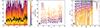 |
Fig. 4. a) Distribution of θ, the angle between the magnetic field and the mean field direction as a function of the solar radius. The black line shows the mean θ at each radius, with a linear least square fit line shown in black. b) Quartiles and 95th percentile of distribution shown in panel (a). Least square fit lines are shown for each percentile. c) Probability of θ > θcrit for a range of θcrit between 15 and 105 degrees. Larger θcrit are shown in lighter colors. Linear least square fit trend lines are plotted for each θcrit. |
In Figure 4(b) we plot quartiles of the distribution of θ from each interval as a function of R as well as the 95th percentile of the distribution of θ. We show a best-fit line to each quartile and the 95th percentile: the distributions systematically move toward higher average values of θ, which is consistent with the growth of the fluctuations from expansion. We also plot the best-fit line to the average θ. Finally, Fig. 4(c) further highlights the growth of SBs by showing, for each interval, the probability that the angle, θ, is larger than a critical angle, θcrit, which is varied from θcrit = 15° to θcrit = 105°. For each θcrit we fit linear best-fit lines. The slopes of the best fit lines clearly show increasing trends, indicating that the probability of θ > θcrit increases with distance. For inversion angles of θ = 90°, there is a very low probability, P(θ < 90 ° ) < 0.1% at 20R⊙, whereas P(θ < 60 ° ) ≈ 1% at 20R⊙. At 55R⊙, P(θ < 90 ° ) ≈ 1% and P(θ < 60 ° ) ≈ 10%. The structure of the least square trend lines, indicating SB growth, are similar to numerical simulations of SB formation via expansion (Johnston et al. 2022).
4. Discussion
Magnetic field inversions have been observed in the heliosphere for many years (McCracken & Ness 1966; Balogh et al. 1999; Gosling et al. 2009). However, recent observations from PSP have brought a significant focus on these structures, their use in constraining solar wind sources (Bale et al. 2023; Raouafi et al. 2023b), and their role in heating the solar corona and wind (Woolley et al. 2020; Laker et al. 2021; Tenerani et al. 2020). Understanding the formation of these structures is fundamental to successfully employing them as a constraint on solar wind sources and understanding their interplay with heating. In this paper, we present evidence that many SBs may be formed in situ via the effects on expansion on large-scale outward propagating Alfvén waves (Squire et al. 2020; Shoda et al. 2021; Mallet et al. 2021; Johnston et al. 2022; Matteini et al. 2024).
Our results suggest that the outer-scale fluctuations are consistent with a population of large-amplitude spherically polarized fluctuations. The stationary frame of the outer-scale fluctuations, measured through the dHT frame, is consistent with the Alfvén speed, suggesting that the large amplitude, constant B structures are likely Alfvén waves propagating away from the sun (Gosling et al. 2009; Matteini et al. 2015) and that they are often found in the near-Sun solar wind (Dunn et al. 2023).
The application of conservation of wave action (Heinemann & Olbert 1980; Chandran & Hollweg 2009) demonstrates that the empirically observed wave amplitudes grow as the solar wind expands. As the waves grow through expansion, the normalized amplitudes increase, leading to greater fractions of the observed fluctuations having amplitudes capable of “switching back” the magnetic field. Importantly, the growth in the amplitudes is not entirely consistent with conservation of wave action, indicating that some energy from the waves must be lost (Chandran & Perez 2019). However, empirical measurement of proton heating rates via deviations from adiabatic expectations (Chew et al. 1956; Zaslavsky 2023; Mozer et al. 2023) reveals levels of proton heating roughly consistent with heating rates obtained from both consideration of conservation wave action at outer scales as well as the turbulent energy flux (Politano & Pouquet 1998). While there are significant uncertainties on calculations of the turbulent cascade rate and heating rates, the general correspondence and similar scalings observed between the dissipated energy, turbulent cascade rate, and proton heating rates suggest that these processes are closely intertwined. These observations are important for understanding the expanding solar wind and suggest that the onset of the turbulent cascade and solar wind heating are important in regulating the growth of SBs. Increased amounts of heating would result in lower growth rates of dB/B, which may inhibit the growth of SBs through expansion. The kinetics of proton heating in this stream were recently studied by Bowen et al. (2024b), in which significant cyclotron resonant resonant was found but partition in ion-electron heating rates was not considered. The observation of Qp/Qe >1 we report here is consistent with cyclotron resonant heating mechanisms as a means of dissipating turbulence previously shown in Bowen et al. (2024a). While we have omitted the electron heat flux, these measurements, which indicate residual electron heating in excess of adiabatic evolution, are consistent with the overall magnitude of heating found by Štverák et al. (2015); however, we have not considered the contribution to the heat flux, which Štverák et al. (2015) found to be larger in magnitude to the Qe that we consider, and which furthermore is negative in sign and thus significantly affects the electron heating. Further analysis of electron heating should use SPAN-e data Halekas (2020) to fully analyze the radial electron distributions and identify the subtleties in the partition of ion and electron heating. Similarly, a number of subtleties exist in the application of CGL (Zaslavsky 2023). Future studies on radial scans of PSP, which can provide an analysis of solar wind evolution in a single stream, are important to understand the connections between specific microphysical heating processes with nonadiabatic evolution of the observed VDFs.
Further work is necessary to consider the in situ development of the SBs through other mechanisms; for instance, the Kelvin Helmholtz instability (KHI), a leading alternative to the in situ development via expansion (Mozer et al. 2020; Ruffolo et al. 2020). Agapitov et al. (2023) have recently studied KHI in the presence of SBs and note that observed SBs seem stable in relation to KHI, though they may be regulated by the instability. Additionally, a significant body of work has discussed the generation of SBs through reconnection much closer to the solar surface Drake et al. (2021), Bale et al. (2021), Fargette et al. (2021), Bale et al. (2023). While our results do not preclude the generation of these features close to the sun, our analysis clearly supports a role of expansion and in situ formation of SBs. Patches of SBs (Bale et al. 2021; Fargette et al. 2021; Shi et al. 2022) have gained particular interest in the community as the modulated patch size seems to correspond to super-granulation scales. If this modulation of the SBs does indeed correspond to features on the solar surface, it remains an important question to understand how the patch-like modulation evolves under expansion and dissipation.
Many open questions remain regarding SBs: their origins, relation to heating, and fundamental relations and impact on solar wind turbulence (Raouafi et al. 2023a). In this brief paper, we have attempted to clearly demonstrate evidence for the natural growth of SBs through expansion. Indeed, the spherically polarized Alfvénic state is an equilibrium solution to the MHD equations and it is certainly possible that many physical processes may inevitably relax to this state.
Acknowledgments
TAB acknowledges support from 80NSSC21K1771. BDGC acknowledges the support of NASA grant 80NSSC24K0171. STB was supported by the Parker Solar Probe project through the SAO/SWEAP subcontract 975569. AM was supported by NASA grants 80NSSC21K0462, 80NSSC24K0272, and NASA contract NNN06AA01C. The PSP/FIELDS experiment was developed and is operated under NASA contract NNN06AA01C. JS acknowledges the support of the Royal Society Te Apārangi, through Marsden-Fund grant MFP-UOO2221. This work was supported by the ISSI “Magnetic Switchbacks in the Young Solar Wind” workshop.
References
- Agapitov, O. V., Drake, J. F., Swisdak, M., Choi, K. E., & Raouafi, N. 2023, ApJ, 959, L21 [Google Scholar]
- Alfvén, H. 1942, Nature, 150, 405 [Google Scholar]
- Badman, S. T., Riley, P., Jones, S. I., et al. 2023, J. Geophys. Res. (Space Phys.), 128, e2023JA031359 [NASA ADS] [CrossRef] [Google Scholar]
- Bale, S. D., Goetz, K., Harvey, P. R., et al. 2016, Space Sci. Rev., 204, 49 [Google Scholar]
- Bale, S. D., Badman, S. T., Bonnell, J. W., et al. 2019, Nature, 576, 237 [NASA ADS] [CrossRef] [Google Scholar]
- Bale, S. D., Horbury, T. S., Velli, M., et al. 2021, ApJ, 923, 174 [NASA ADS] [CrossRef] [Google Scholar]
- Bale, S. D., Drake, J. F., McManus, M. D., et al. 2023, Nature, 618, 252 [NASA ADS] [CrossRef] [Google Scholar]
- Balogh, A., Forsyth, R. J., Lucek, E. A., Horbury, T. S., & Smith, E. J. 1999, Geophys. Res. Lett., 26, 631 [Google Scholar]
- Bandyopadhyay, R., Meyer, C. M., Matthaeus, W. H., et al. 2023, ApJ, 955, L28 [Google Scholar]
- Barnes, A., & Hollweg, J. V. 1974, JGR, 79, 2302 [Google Scholar]
- Belcher, J. W., & Davis, L., Jr 1971, J. Geophys. Res., 76, 3534 [NASA ADS] [CrossRef] [Google Scholar]
- Berčič, L., Larson, D., Whittlesey, P., et al. 2020, ApJ, 892, 88 [Google Scholar]
- Bowen, T. A., Bale, S. D., Chandran, B. D. G., et al. 2024a, Nat. Astron., 8, 482 [Google Scholar]
- Bowen, T. A., Vasko, I. Y., Bale, S. D., et al. 2024b, ApJ, 972, L8 [Google Scholar]
- Bowen, T. A., Dunn, C. I., Mallet, A., et al. 2025, ApJ, 985, 49 [Google Scholar]
- Chandran, B. D. G., & Hollweg, J. V. 2009, ApJ, 707, 1659 [Google Scholar]
- Chandran, B. D. G., & Perez, J. C. 2019, J. Plasma Phys., 85, 905850409 [NASA ADS] [CrossRef] [Google Scholar]
- Chandran, B. D. G., Quataert, E., Howes, G. G., Hollweg, J. V., & Dorland, W. 2009, ApJ, 701, 652 [Google Scholar]
- Chew, G. F., Goldberger, M. L., & Low, F. E. 1956, Proc. R. Soc. London Ser. A, 236, 112 [NASA ADS] [CrossRef] [Google Scholar]
- Cranmer, S. R., Matthaeus, W. H., Breech, B. A., & Kasper, J. C. 2009, ApJ, 702, 1604 [Google Scholar]
- Davis, N., Chandran, B. D. G., Bowen, T. A., et al. 2023, ApJ, 950, 154 [NASA ADS] [CrossRef] [Google Scholar]
- Drake, J. F., Agapitov, O., Swisdak, M., et al. 2021, A&A, 650, A2 [EDP Sciences] [Google Scholar]
- Dudok de Wit, T. 2004, Phys. Rev. E, 70, 055302 [Google Scholar]
- Dudok de Wit, T., Krasnoselskikh, V. V., Bale, S. D., et al. 2020, ApJS, 246, 39 [Google Scholar]
- Dunn, C., Bowen, T. A., Mallet, A., Badman, S. T., & Bale, S. D. 2023, ApJ, 958, 88 [NASA ADS] [CrossRef] [Google Scholar]
- Fargette, N., Lavraud, B., Rouillard, A. P., et al. 2021, ApJ, 919, 96 [NASA ADS] [CrossRef] [Google Scholar]
- Goldstein, M. L., Klimas, A. J., & Barish, F. D. 1974, in Solar Wind Three, ed. C. T. Russell, 385 [Google Scholar]
- Gosling, J. T., McComas, D. J., Roberts, D. A., & Skoug, R. M. 2009, ApJ, 695, L213 [Google Scholar]
- Halekas, J., et al. 2020, ApJS [Google Scholar]
- Halekas, J. S., Bale, S. D., Berthomier, M., et al. 2023, ApJ, 952, 26 [Google Scholar]
- Heinemann, M., & Olbert, S. 1980, J. Geophys. Res., 85, 1311 [Google Scholar]
- Hollweg, J. V. 1974, JGR, 79, 1539 [Google Scholar]
- Horbury, T. S., Woolley, T., Laker, R., et al. 2020, ApJS, 246, 45 [Google Scholar]
- Huang, Z., Sioulas, N., Shi, C., et al. 2023, ApJ, 950, L8 [NASA ADS] [CrossRef] [Google Scholar]
- Johnston, Z., Squire, J., Mallet, A., & Meyrand, R. 2022, Phys. Plasmas, 29, 072902 [NASA ADS] [CrossRef] [Google Scholar]
- Kasper, J. C., Abiad, R., Austin, G., et al. 2016, Space Sci. Rev., 204, 131 [Google Scholar]
- Kasper, J. C., Bale, S. D., Belcher, J. W., et al. 2019, Nature, 576, 228 [Google Scholar]
- Khrabrov, A. V., & Sonnerup, B. U. Ö. 1998, ISSI Sci. Rep. Ser., 1, 221 [NASA ADS] [Google Scholar]
- Klein, K. G., Verniero, J. L., Alterman, B., et al. 2021, ApJ, 909, 7 [NASA ADS] [CrossRef] [Google Scholar]
- Laker, R., Horbury, T. S., Bale, S. D., et al. 2021, A&A, 650, A1 [EDP Sciences] [Google Scholar]
- Larosa, A., Krasnoselskikh, V., DudokdeWit, T., et al. 2021, A&A, 650, A3 [NASA ADS] [CrossRef] [EDP Sciences] [Google Scholar]
- Lichtenstein, B. R., & Sonett, C. P. 1980, GRL, 7, 189 [Google Scholar]
- Livi, R., Larson, D. E., Kasper, J. C., et al. 2022, ApJ, 938, 138 [NASA ADS] [CrossRef] [Google Scholar]
- Mallet, A., Squire, J., Chandran, B. D. G., Bowen, T., & Bale, S. D. 2021, ApJ, 918, 62 [NASA ADS] [CrossRef] [Google Scholar]
- Marsch, E., Muehlhaeuser, K. H., Rosenbauer, H., & Schwenn, R. 1983, J. Geophys. Res., 88, 2982 [Google Scholar]
- Matteini, L., Horbury, T. S., Pantellini, F., Velli, M., & Schwartz, S. J. 2015, ApJ, 802, 11 [Google Scholar]
- Matteini, L., Tenerani, A., Landi, S., et al. 2024, Phys. Plasmas, 31, 032901 [NASA ADS] [CrossRef] [Google Scholar]
- McCracken, K. G., & Ness, N. F. 1966, JGR, 71, 3315 [Google Scholar]
- Moncuquet, M., Meyer-Vernet, N., Issautier, K., et al. 2020, ApJS, 246, 44 [Google Scholar]
- Mozer, F. S., Agapitov, O. V., Bale, S. D., et al. 2020, ApJS, 246, 68 [Google Scholar]
- Mozer, F. S., Agapitov, O. V., Kasper, J. C., et al. 2023, A&A, 673, L3 [NASA ADS] [CrossRef] [EDP Sciences] [Google Scholar]
- Perrone, D., Stansby, D., Horbury, T. S., & Matteini, L. 2019, MNRAS, 483, 3730 [Google Scholar]
- Politano, H., & Pouquet, A. 1998, Geophys. Res. Lett., 25, 273 [NASA ADS] [CrossRef] [Google Scholar]
- Pulupa, M., Bale, S. D., Bonnell, J. W., et al. 2017, J. Geophys. Res. (Space Phys.), 122, 2836 [NASA ADS] [CrossRef] [Google Scholar]
- Raouafi, N. E., Matteini, L., Squire, J., et al. 2023a, Space Sci. Rev., 219, 8 [NASA ADS] [CrossRef] [Google Scholar]
- Raouafi, N. E., Stenborg, G., Seaton, D. B., et al. 2023b, ApJ, 945, 28 [NASA ADS] [CrossRef] [Google Scholar]
- Riley, P., Sonett, C. P., Tsurutani, B. T., et al. 1996, JGR, 101, 19987 [Google Scholar]
- Rivera, Y. J., Badman, S. T., Stevens, M. L., et al. 2024, Science, 385, 962 [NASA ADS] [CrossRef] [Google Scholar]
- Ruffolo, D., Matthaeus, W. H., Chhiber, R., et al. 2020, ApJ, 902, 94 [Google Scholar]
- Shi, C., Panasenco, O., Velli, M., et al. 2022, ApJ, 934, 152 [CrossRef] [Google Scholar]
- Shoda, M., Chandran, B. D. G., & Cranmer, S. R. 2021, ApJ, 915, 52 [CrossRef] [Google Scholar]
- Squire, J., Chandran, B. D. G., & Meyrand, R. 2020, ApJ, 891, L2 [Google Scholar]
- Štverák, Š., Trávníček, P. M., & Hellinger, P. 2015, J. Geophys. Res. (Space Phys.), 120, 8177 [CrossRef] [Google Scholar]
- Tenerani, A., Velli, M., Matteini, L., et al. 2020, ApJS, 246, 32 [Google Scholar]
- Woolley, T., Matteini, L., Horbury, T. S., et al. 2020, MNRAS, 498, 5524 [Google Scholar]
- Zaslavsky, A. 2023, GRL, 50, e2022GL101548 [Google Scholar]
All Figures
|
Fig. 1. a) FIELDS magnetic field data in RTN coordinates. The magnitude, |B|, is shown in black. b) Radial component of magnetic field normalized to field magnitude BR/|B|. Large-scale inversions in BR known as SBs are observed. c) SWEAP SPAN velocity measurements in RTN coordinates. |V| is shown in black. d) Computed dHT frame speed, VdHT, Alfvén speed, VA, and average wind speed, Vsw, and η = (VA/Vsw)2. |
| In the text | |
|
Fig. 2. a) Root mean squared dB, dB⊥, and dB∥ (black, maroon, red); magnitude of the mean magnetic field, B0, orange. b) Spherically confined fluctuations, dB, dB⊥, and dB∥, (black, maroon, red) where all fluctuations maintain a constant magnitude, |Bsph|. The RMS residual fluctuations between the total field and spherically polarized field, dBC, are shown in dark blue. The dashed red line shows the wave amplitude from conservation of wave action with no dissipation. The blue line shows the best fit to dBsph. c) Normalized amplitudes, dB⊥sph/B0, dB∥sph/B0, and |
| In the text | |
|
Fig. 3. a) Radial scaling of dissipation rates computed from WKB expansion of outer scale fluctuations, Q (black), from Chandran et al. (2009), CGL estimate of proton heating, Qp (yellow), following Zaslavsky (2023), third-order cascade rate, ϵ (Politano & Pouquet 1998), and electron heating, Qe (Cranmer et al. 2009). Solid lines show the moving-window median value. b) Ratios of dissipation quantities, ϵ/Q (red), Qp/Q (yellow), Qp⊥/Qp (black), and Qp∥/Qp (purple). c) PDFs of ratios Qp/Q (yellow), ϵ/Q (red), ϵ/Qp (orange), and Qp/Qe (purple). |
| In the text | |
|
Fig. 4. a) Distribution of θ, the angle between the magnetic field and the mean field direction as a function of the solar radius. The black line shows the mean θ at each radius, with a linear least square fit line shown in black. b) Quartiles and 95th percentile of distribution shown in panel (a). Least square fit lines are shown for each percentile. c) Probability of θ > θcrit for a range of θcrit between 15 and 105 degrees. Larger θcrit are shown in lighter colors. Linear least square fit trend lines are plotted for each θcrit. |
| In the text | |
Current usage metrics show cumulative count of Article Views (full-text article views including HTML views, PDF and ePub downloads, according to the available data) and Abstracts Views on Vision4Press platform.
Data correspond to usage on the plateform after 2015. The current usage metrics is available 48-96 hours after online publication and is updated daily on week days.
Initial download of the metrics may take a while.