| Issue |
A&A
Volume 700, August 2025
|
|
|---|---|---|
| Article Number | A144 | |
| Number of page(s) | 15 | |
| Section | Interstellar and circumstellar matter | |
| DOI | https://doi.org/10.1051/0004-6361/202452044 | |
| Published online | 15 August 2025 | |
Metallic species in the interstellar medium: Astrochemical modeling
1
Max-Planck-Institute for extraterrestrial Physics,
PO Box 1312,
85741
Garching,
Germany
2
Institute of Astronomy Space and Earth Science,
P177 CIT Road, Scheme 7m,
Kolkata
700054,
India
3
Univ. Grenoble Alpes, CNRS, IPAG,
38000
Grenoble,
France
4
Univ Rennes, CNRS, IPR (Institut de Physique de Rennes) – UMR 6251,
35000
Rennes,
France
★ Corresponding authors: This email address is being protected from spambots. You need JavaScript enabled to view it.
; This email address is being protected from spambots. You need JavaScript enabled to view it.
Received:
29
August
2024
Accepted:
17
June
2025
Abstract
Metal-bearing species in diffuse or molecular clouds are often overlooked in astrochemical modeling except for the charge exchange process. However, catalytic cycles involving these metals can affect the abundance of other compounds. We prepared a comprehensive chemical network for Na, Mg, Al, Fe, K, and Si-containing species. Assuming water as the major constituent of interstellar ice in dark clouds, quantum chemical calculations were carried out to estimate the binding energy of important metallic species, considering amorphous solid water as the substrate. Significantly lower binding energies (approximately five to six times) were observed for Na and Mg, while the value for Fe was roughly four times higher than what was used previously. Here, we calculated binding energy values for Al and K, for which no prior guesses were available. The obtained binding energies are directly implemented into the models of diverse interstellar environments. The total dipole moments and enthalpies of formation for several newly included species are unknown. Furthermore, the assessment of reaction enthalpies is necessary to evaluate the feasibility of the new reactions under interstellar conditions. These parameters were estimated and subsequently integrated into models. Some additional species that were not included in the UMIST/KIDA database have been introduced. The addition of these new species, along with their corresponding reactions, appears to significantly affect the abundances of related species. Some key reactions that significantly influence general metal-related chemistry include: M+ + H2 → MH+2 + hv, MH + O → MO + H (M = Fe, Na, Mg, Al, or K), and M+1 + M2H → M1H + M+2 (where M1 ≠ M2, M1, M2 = Na, Mg, Al, K, Fe). These reactions have a notable impact on the abundance of these species. Significant changes were observed in magnesium and sodium-bearing cyanides, isocyanides, and aluminum fluoride when additional reaction pathways were considered.
Key words: astrochemistry / ISM: abundances / ISM: clouds / dust, extinction / ISM: molecules / photon-dominated region (PDR)
© The Authors 2025
 Open Access article, published by EDP Sciences, under the terms of the Creative Commons Attribution License (https://creativecommons.org/licenses/by/4.0), which permits unrestricted use, distribution, and reproduction in any medium, provided the original work is properly cited.
This article is published in open access under the Subscribe to Open model.
Open Access funding provided by Max Planck Society.
1 Introduction
Almost 90% of all refractory elements condense in the innermost envelopes of evolved stars. The condensation occurs at the condensation temperature of the ingredients. So, it is expected that dust grains are layered based on the highest-lowest condensation sequence in the following order: Al, Ti, Ca, Fe, (Mg, Si), P, (Na, K), and S (Turner 1992). The chemistry associated with the metals is important in magnetized clouds because metals play a crucial role in regulating the ionization fraction of the interstellar medium (ISM). However, their identification in space is limited due to the lack of spectroscopic information and weak transitions in the radio domain. Nevertheless, a handful of metallic compounds have been identified to date. It includes multiple metallic halides (NaCl, AlCl, KCl, and AlF; Cernicharo & Guelin 1987), metal cyanides (MgCN, KCN, SiCN, NaCN, FeCN, MgC3N; Ziurys et al. 1995; Pulliam et al. 2010; Guélin et al. 2000; Turner et al. 1994; Zack et al. 2011; Cernicharo et al. 2019a), metal isocyanides (MgNC, CaNC, SiNC, AlNC, HMgNC; Guelin et al. 1993; Cernicharo et al. 2019b; Guélin et al. 2004; Ziurys et al. 2002; Cabezas et al. 2013), etc. The IRC+10216, circumstellar envelope (CSE) of the carbon-rich star, is a major inventory of these species found to date. In addition, some species were also located toward the more evolved carbon star CRL 2688 (Highberger et al. 2003).
Metal oxides can be detected in the atmosphere of stars. However, it is challenging to identify refractory elements, such as Mg, Fe, Ca, and Si, in molecular clouds due to their high degree of depletion. While SiO has been observed along multiple lines of sight, its abundance is several orders of magnitude lower than the solar abundance of Si. Typically, SiO can be found in regions of shocks or outflows. The absorption of the J = 5 - 4 transition of FeO has been observed toward Sgr B2(M) by Walmsley et al. (2002) and Furuya et al. (2003).
Recently, NaCl has been detected in the massive protostellar system, Orion Source I disk (Ginsburg et al. 2019; Wright et al. 2020). Also, Tanaka et al. (2020) find NaCl, SiO, and SiS emissions in the inner disk (~ 100 au scale) of a massive protostellar disk, IRAS 16547-4247. Most interestingly, all these emissions do not necessarily have very high upper-state energy, and critical densities are also not too high (105−106 cm−3). Identifying these refractory species in the innermost region of massive protostellar disks may be the product of dust destruction, which may be feasible around the inner disk. Moreover, Al, Na, and K metalbearing species are closed-shell molecules, mainly obtained in the hotter part of the envelope. On the contrary, Mg, Si, and Fe-related species are mostly open-shell radicals that may react in cold environments.
The C-rich envelope of evolved stars is well explored by earlier studies (Cernicharo 2012; Agúndez & Wakelam 2013). Here, we focus mainly on metallic compounds in the ISM. We studied various star-forming regions where the formation of metallic species is often overlooked. Our focus includes harsh environments that are conducive to molecular formation, such as the HII, photodissociation region (PDR). We also examined ultraviolet (UV) radiation-shielded areas that are favorable for forming complex species. These areas include diffuse clouds, dark clouds, and hot core regions. An extensive chemical network for the metallic species was prepared and then coupled with the existing chemical network. Quantum chemical calculations were conducted to study various chemical properties (reaction enthalpies, binding energies, dipole moments, etc.). The examination of metal-bearing species in other star-forming regions falls outside the scope of this paper; however, the pathways and chemical parameters presented here are likely applicable in a broader context.
This paper is organized as follows. First, in Sect. 2, we explain the results of physical chemistry, including the estimation of binding energies, the molecular dipole moments of the species studied, and the reaction enthalpies for the newly included reactions. In Sect. 3, we discuss the chemical routes for gas and ice-phase metallic compounds. Sect. 4 presents an in-depth discussion of the various chemical models used in this work. Sect. 5 covers the results and their astrophysical implications. Finally, we conclude in Sect. 6.
2 Physical chemistry results
2.1 Binding energy
Among the six metallic elements (Na, Mg, Si, Al, K, and Fe) considered here, the binding energy calculation of only Si was available (~11600 ± 3480 K; Wakelam et al. 2017). For Na, Mg, and Fe, the KIDA database noted the binding energy as 11 800 K, 5300 K, and 4200 K, respectively, estimated from very early studies (the OSU database of Eric Herbst in 2006). However, no follow-up studies supported these estimates via quantum chemical calculations or experiments (Penteado et al. 2017; Das et al. 2018). Das et al. (2018) obtain binding energies on water tetramer using MP2/aug-cc-pVDZ level of theory without considering ZPE-correction. Penteado et al. (2017) provide average binding energies based on the work of Hasegawa & Herbst (1993) and Aikawa et al. (1996) with an uncertainty set to 500 K.
Since the depletion of heavy elements could control the ionization of the medium and, eventually, the star formation rate, it is beneficial to have a better understanding of the binding energy of these metals. Here, we performed the quantum chemical calculations to determine the binding energy of some of these key species noted in Table 1. We used the MP2/aug-cc-pVDZ level of theory (Dunning 1989) without considering ZPE correction (Das et al. 2018; Das et al. 2021; Sil et al. 2017) for BE computations with water monomer. A scaling factor of 1.416 (in case of monomer; Das et al. 2018) was used. Since the aug-cc-pVDZ basis set is not supported for the K-related species, we used the MP2/Def2-TZVPP level of theory (Weigend & Ahlrichs 2005) without considering ZPE corrections (the same scaling factor of 1.416 was used). For water tetramer surfaces (in a few cases), we used the MP2/Def2-TZVPP level of theory, considering ZPE corrections to predict the binding energies (no scaling factor was used). We must admit that the vast astrophysical environments modeled here would not have water as a substrate, and the interaction with other substrates would differ significantly. However, a systematic study based on a single substrate would be better than arbitrary guesses. The computation of binding energy with other substrates is out of the scope of this paper and will be reported elsewhere. First, the ground state spin multiplicity of the species was verified by reviewing the optimized energies. Then, the ground state spin multiplicity considered in this study is noted in Table 1. Our calculated binding energy of Si of 7187 K with water monomer is toward the lower limit range provided by Wakelam et al. (2017). Interestingly, we obtained very low binding energy values for Na (2408 K) and Mg (860 K) with the water tetramer compared to the available literature values. For the other metals, Al, Fe, and K, we obtained binding energy values of 4381 K, 16 677 K, and 2133 K, respectively. We proposed calculated binding energies for the elements Al and K, for which no previous estimates were available. We used a diffusion (Eb) to desorption (ED) energy ratio of 0.5 for all the models considered here.
2.2 Reaction enthalpies
Apart from the standard gas-phase reactions (Millar et al. 2024), Table A.1 (available on Zenodo) presents some additional gasphase reactions studied in this work. The reaction enthalpies [ΔrH0(298 K)] for some reactions were calculated to evaluate their validity under interstellar conditions. Although these reaction enthalpies were computed at 298 K, we note that the differences in reaction enthalpies between 298 K and typical dark cloud temperatures (~10 K) are expected to be negligible, as enthalpy is only weakly temperature-dependent over this range. The main factors influencing reactivity in such low-temperature environments are instead kinetic (e.g., activation barriers) rather than thermodynamic. The exothermic reactions are highlighted in Table A.1 (available on Zenodo) and are finally included in our gas-phase chemical network. The typical method for calculating reaction enthalpies involves determining the heat of formation and applying the appropriate sums and differences mentioned below:
 (1)
(1)
The atomization energy of molecules was calculated using the DFT-B3LYP/6-311+G(d,p) method to determine the enthalpy of formation. All the quantum chemical calculations conducted in this work were performed utilizing the Gaussian 16 computational program (Frisch et al. 2016). Experimental data for the heat of formation of atoms was obtained from Curtiss et al. (1997). Table A.2 summarizes the standard enthalpy of formation [ΔrH0(298 K)] for the species considered. Most values were sourced from the NIST Chemistry WebBook, SRD 69 gasphase thermochemistry database. However, in cases where the enthalpies of formation are not available in the literature, or we could not determine it due to lack of experimental data of constituent atoms, we simply took the difference of the sums of electronic and thermal enthalpies for the reactants and the products calculated using the DFT-B3LYP/6-311+G(d,p) level of theory.
2.3 Dipole moment
Ion-neutral reactions play a crucial role in the ISM (Herbst & Klemperer 1973). These reactions often proceed rapidly at low temperatures, influencing the chemical evolution of molecular clouds.
We used the approximated Su & Chesnavich (1982) formula as prescribed by Millar et al. (2024) to calculate ion-neutral (IN) rate coefficients:
 (2)
(2)
where μD is the electric dipole moment of the neutral species in Debye, and μ is the reduced mass of the reactants in amu. Dipole moments for some of the metallic species considered in our network were not available, and thus, we employed quantum chemical calculations to estimate it with the DFT-B3LYP/6-311+G(d,p) level of theory. Table 2 denotes the dipole moment used in our calculations.
Computed binding energies of metal-bearing species considering water monomer (default) as the substrate while incorporating a scaling factor of 1.416 (see text for details).
3 Chemical routes
This study uses two state-of-the-art astrochemical codes: The Cloudy photoionization code version 22.01 (Ferland et al. 2017; Shaw et al. 2022), and two phase Chemical Model for Molecular Cloud code (CMMC; Das et al. 2015a; Sil et al. 2018; Das et al. 2019; Das et al. 2021; Sil et al. 2021; Bhat et al. 2022; Gorai et al. 2017, 2020; Mondal et al. 2021; Ghosh et al. 2022; Srivastav et al. 2022; Ramachandran et al. 2024).
3.1 Gas-phase pathways
Some essential charge transfer reactions related to Na, Mg, and Si are already considered in the Cloudy code from McElroy et al. (2013). However, the CMMC code considered all the charge transfer reactions of these species noted in the UMIST-2022 database for Astrochemistry (Millar et al. 2024). Fe-related charge transfer reactions are not considered in the Cloudy code, but they were considered in the CMMC code from UMIST. We incorporated the charge transfer reactions of these species in both codes as considered in Millar et al. (2024). Our study includes additional Al and K-related charge exchange reactions by considering a similar charge exchange reaction analogous to Fe and Na, respectively. Since not too many negative ions were considered in the Cloudy network, we only limited our consideration to some essential negative ions. However, we already considered all the reactions with the negative ions from UMIST-2022 in the CMMC code for Na, Mg, Fe, and Si. Table A.1 (available on Zenodo) presents the newly included gas-phase reactions in this study. As discussed in Sect. 2.2, we calculated the enthalpies of several reactions; however, only exothermic reactions were included in our gas-phase network. Furthermore, the adopted rate and the proxy metal used instead are clearly highlighted for reference.
Total dipole moment for the species considered in our model.
3.2 Grain surface reactions
In the CMMC code, we considered an extensive network of grain surfaces. This network is primarily based on the network provided by Ruaud et al. (2016). It also considers the H-abstraction reactions proposed by Belloche et al. (2014) and Garrod et al. (2017). However, in Cloudy, we selectively included some surface reactions relevant to this study.
Apart from the various essential surface reactions considered in the CMMC code, the following are important grain surface reactions relevant to this work. These reactions were also included in the Cloudy network. It is important to note that the Cloudy network includes very limited grain surface chemistry, and therefore, we did not utilize this code in scenarios where molecular depletion is significant and surface chemistry is crucial.
Sigr + Hgr → SiHgr,
SiHgr + Hgr → SiH2gr,
SiH2gr + Hgr → SiH3gr,
SiH3gr + Hgr → SiH4gr,
Nagr + Hgr → NaHgr,
Fegr + Hgr → FeHgr,
Mggr + Hgr → MgHgr,
MgHgr + Hgr → MgH2gr,
Kgr + Hgr → KHgr,
Algr + Hgr → AlHgr,
Nagr + Clgr → NaClgr,
Nagr + Sgr → NaSgr,
Kgr + Clgr → KClgr,
NaHgr + Clgr → NaClgr+Hgr1
Moreover, we considered cosmic-ray-induced desorption and photo-desorption of these species. Since the cosmic-ray-induced desorption and photo-dissociation rates were given for some of the Si-related species, we considered a similar rate for the other metallic compounds considered in our network for simplicity.
4 Chemical models for various regions
We utilized Cloudy v22.01 to model the H II-PDR. Due to its ability to consider various microphysics, the Cloudy code is useful in studying chemical compositions of H II-PDR (Das et al. 2020; Sil et al. 2024a, 2025). Additionally, we employed the CMMC code to model the diffuse cloud, dark cloud, and hot core regions. For the gas-phase chemistry, Cloudy v22.01 was based on the UMIST-2012 database (McElroy et al. 2013), while the CMMC code used the UMIST-2022 gas-phase network (Millar et al. 2024). It’s worth noting that Cloudy did not consider grain surface reactions extensively, whereas the CMMC code employed an extensive grain surface chemical network.
4.1 HII region and PDR
HII regions are created when the extreme UV radiation from a young massive star emits copious amounts of photons beyond the Lyman limit (hν > 13.6 eV) and ionizes and heats its surrounding molecular cloud. The PDR is often associated with the H II region. A PDR is a neutral atomic region where the column density of the cloud is insufficient to block the far-UV photon (6 eV < hν < 13.6 eV). These far-UV photons are the primary energy sources to glow this region in the infrared (IR) and regulate various chemical processes crucial for star formation in galaxies (Hollenbach & Tielens 1997). Atomic hydrogen is the most abundant here, but a little deeper inside the cloud, where the UV radiation field is attenuated, the formation of molecular hydrogen starts. Similarly, the transition of C+ to CO begins around this region. Here, we used the models by Abel et al. (2005); Shaw et al. (2022) to self-consistently model the thermal and chemical structure of the HII and PDR. We adopted the non-LTE CoStar stellar atmospheres with a temperature of the ionizing star (T★) ~39 600 K, numbers of ionizing photons per second (Q(H)) ~1049, and a photon flux of per unit area of cloud surface (Φ(H)) ~10 cm−2s−1. The separation between the star and the cloud inner surface of ~2.82 × 1017 cm with a closed geometry was considered for this calculation. A gas-phase abundance based on average abundances obtained in the Orion Nebula was used (Baldwin et al. 1996; Abel et al. 2005). We considered a Galactic cosmic-ray ionization rate having a mean H0 ionization rate (ζH) of 2.0 x 10⁻¹⁶ s−1. Since a few grain surface reactions were included in the Cloudy v22.01, we stopped our calculations at AV = 5.5 mag to avoid misleading results. We used the initial elemental abundances listed in the second column of Table 3. These are the abundances for the HII region, such as the Orion Nebula (Baldwin et al. 1991; Osterbrock et al. 1992; Rubin et al. 1993). Na, K, and Al were not considered in the model of Shaw et al. (2022) and Abel et al. (2005). We considered an initial elemental abundance of Na, K, and Al of 3.0 x 10⁻⁷, 1.1 x 10⁻⁸, and 2.00 x 10⁻⁷, respectively. The MRN size distribution (Mathis et al. 1977) was used with amin = 0.03 μm and amax = 0.25 μm to produce the Orion extinction curve around RV = 5.5 (Baldwin et al. 1996). With this grain size distribution, we obtained RV = 5.32.
In Fig. 1, the upper panel displays variations in number density (hydrogen and electron) and temperature with visual extinction, while the lower panel shows the variation in abundance for different H, C, and O species. A closed geometry was considered with a central star surrounded by a cloud ring. The increase in visual extinction on the right side indicates that the left side is the illuminated face. The two red dashed vertical lines in the figure indicate the PDR starting from the boundary of the HII region (ionization front (IF) where half of the H+ has recombined) up to the H/H2 transition zone (dissociation front (DF) where molecular hydrogen number density reaches 50% of the number density of total hydrogen nuclei).
According to the data presented in the lower panel, at the beginning of the PDR, all the H+ ions are transformed into atomic H, and O+ is converted into atomic O. Carbon, on the other hand, remains largely in C+ form. As we move toward the deeper parts of the cloud (AV > 5), the formation of H2 and CO begins. Over time, H2 and CO become some of the most abundant molecules inside the cloud.
Since the Cloudy code does not consider substantial surface chemistry, we restricted our simulation to AV = 5.5. The fate of these molecules in the UV-shielded region is discussed later using the CMMC code for the diffuse, dark, and hot core region in Sections 4.2, 4.3, and 4.4, respectively.
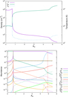 |
Fig. 1 Upper panel: total hydrogen number density, electron number density, and temperature variation. Lower panel: abundance variation of various H, C, and O-related species with respect to total hydrogen nuclei in the HII to PDR obtained from the Cloudy code. |
Initial elemental abundances considered for the H II-PDR, diffuse clud, dark cloud, and hot core cloud models with respect to total hydrogen nuclei.
4.2 Diffuse cloud
We adopted standard solar initial elemental abundances as described by Asplund et al. (2009). Initially, all hydrogen was considered in its atomic form. The species listed in the third column of Table 3 are regarded as ionized if their ionization potential is lower than that of hydrogen. A similar set of elemental abundances is also used by Chantzos et al. (2020) for the diffuse cloud. The only differences are the inclusion of ionized aluminum and potassium in the initial elemental abundance and the consideration of initial fluorine in its neutral form, given its high ionization potential compared to hydrogen.
In this study, we utilized the CMMC code and assumed a total hydrogen nuclei number density (nH) of 500 cm−3 , with an extinction value of 2 mag and a gas temperature of Tgas = 40 K. Similar physical parameters are used by Chantzos et al. (2020) and Sil et al. (2021) in their diffuse cloud models. Recent studies (Obolentseva et al. 2024; Neufeld et al. 2024) have suggested that the gas densities in the foreground interstellar clouds responsible for the observed C2 absorption are a factor of four to seven times smaller than previously inferred. Based on this finding, the consideration of nH = 500 cm−3 for the number densities of local diffuse clouds may be an overestimate. Therefore, we examined an alternative case for the diffuse cloud with nH = 50 cm−3 . Dust temperature was derived from the value of AV using the empirical relation developed by Garrod & Pauly (2011). For AV = 2, the derived dust temperature is approximately 17 K. We used a cosmic-ray ionization rate (ζCR) 1.7 × 10⁻¹⁶ s−1 as was derived by Indriolo et al. (2012). Nonthermal desorption is crucial for exchanging chemical components between gas and grain. We considered the reactive desorption of surface species, leading to a single product (Garrod et al. 2007). The energy released by the reaction was calculated from the difference between the enthalpies of formation of the products and reactants. Our calculated enthalpies of formation (see Table A.2) were used in this estimation. The photodesorption yields of pure CO ice were determined to be 3 × 10⁻³ molecules per UV (7 - 10.5 eV) photon at 15 K in an experimental study by Öberg et al. (2007). A significantly higher photodesorption yield of CO molecules, exceeding the former by a factor of ten, is noted by Muñoz Caro et al. (2010). In our model, we adopted a photodesorption yield of 3 × 10⁻³ molecules photon−1 for all species. The photodesorption rate was estimated using the empirical relation in Öberg et al. (2009).
4.3 Dark cloud
For the dark cloud model, we considered nH = 2 × 104 cm−3, a gas temperature of 10 K, a dust temperature of 10 K, and AV = 10. Following Millar et al. (2024), an initial low metallic depleted elemental abundance shown in the sixth column of Table 3 was considered for the modeling. Asplund et al. (2009) obtain a solar abundance of Al and K as 2.82 × 10⁻⁶ and 1.07 × 10⁻⁷, respectively. Elements like Al suffer from heavy depletion. In diffuse clouds, it is suggested that 90-99% of Al could be depleted into grains (Turner 1991). Considering the same depletion factor for Al as Fe (~10 540 times lower than the solar abundance), we started with an initial Al-abundance of 2.67 X 10⁻¹⁰. Similarly, for the initial elemental abundance of K, we used the same depletion factor as it was considered for Na (~870 times lower than the solar abundance). So, here we started with an initial K-abundance of 1.23 X 10⁻¹⁰. A standard H2 cosmic-ray ionization rate of 1.3 X 10⁻¹⁷ s−1 was considered. We used the CMMC code for this case and continued our simulation for 106 years. The other chemical parameters are the same as in Sect. 4.2.
4.4 Hot core
Here, we considered the CMMC code to model the hot core region. The construction of a toy model for this region was delineated into four distinct phases. The first phase is characterized by a quasi-static collapse, wherein the hydrogen number density of the cloud experiences a linear increase from 3 × 103 cm−3 at t = 0 to 2 × 104 cm−3 at t = 106 years. Concurrently, a linear rise in the extinction value (AV) was assumed, progressing from 2 to 10 mag during this timeframe. The gas temperature (Tgas) was maintained at a steady value of 10 K, while the dust temperature (Tdust) was varied according to the relation presented by Garrod & Pauly (2011); Zucconi et al. (2001). A minimum dust temperature of 10 K was set for this phase.
In the subsequent phase (free-fall collapse phase), the density increases from 2 × 104 cm−3 to 107 cm−3 throughout approximately 3.58 × 10⁵ years following the modified free-fall collapse described in Rawlings et al. (1992). During this stage, it was assumed that the gas and dust temperatures remain well coupled, sustaining a constant temperature of 10 K. The visual extinction parameter increases following the relationship:

where nH0 and AV0 correspond to the initial density ~ 3 × 103 cm−3 and visual extinction ~2 mag established at the onset of the quasi-static collapse phase.
The third phase, the warm-up stage, maintains the density and visual extinction at their maximum levels attained at the end of the free-fall phase, specifically at t = 1.358 × 10⁶ years. During this interval, the gas and dust temperatures are permitted to rise linearly, reaching up to 400 K over 5 × 10⁴ years, ending at t = 1.363 × 10⁶ years. The final stage extends for an additional 105 years, during which the density, temperature, and visual extinction parameters are upheld at their peak values established during the warm-up stage.
We used the initial elemental abundances presented in the eighth column of Table 3 for our modeling. These initial abundances are the same as those considered in Garrod et al. (2017); Srivastav et al. (2022); Ramachandran et al. (2024), except for the initial elemental abundance of Al and K. For Al, we used the same initial elemental abundance (~2.67 × 10⁻¹⁰) as in Sect. 4.3, following the same depletion factor of Fe from its solar abundance. Although Garrod et al. (2017) and Srivastav et al. (2022) used an order of magnitude higher initial elemental abundance of Na (2X 10⁻⁸) than Wakelam et al. (2017, 2 × 10⁻⁹), we adopted an abundance of K of 1.23 × 10⁻¹⁰ for the hot core model. We used a similar abundance of F (approximately 2 × 10⁻⁸) as considered in our dark cloud model. Figure 2 shows the physical parameters and timescales used in our modeling.
5 Results obtained and astrophysical implications
Extensive searches for metallic compounds in diffuse and molecular clouds have been conducted. However, many of these searches have been unsuccessful due to the depletion of refractory elements. It is commonly believed that shocks primarily release refractory elements, which might be present in the molecular cloud, albeit at a low level. In molecular clouds, detailed metal-related chemistry is usually not considered in the chemical network. However, the UMIST-2022 database has recently updated many such reactions. We added some more reactions noted in Table A.1 (available on Zenodo) in the gasphase network to provide a complete list of reactions that could be included. Implementing these additional pathways discussed in Sect. 3 could significantly impact the abundances of metal-related species, which may subsequently alter the abundances of their related species.
The modeled abundances of specific metallic species, those that may be observable and exceed levels of 10−14 relative to H nuclei, are presented for PDRs in Table B.1. For the diffuse, dense, and hot core models, the obtained abundances with our network and with the UMIST-2022 network are shown in Tables B.2, B.3, and B.4, respectively, with levels exceeding 10−12 relative to H2. In these tables, we also included references for earlier observations, along with their estimated abundances or upper limits for these regions. According to our modeling results, the abundance profiles of notable metal-bearing species are shown in Figures 3, 4, 5, and 6 for the PDRs, diffuse clouds, dark clouds, and hot cores, respectively.
In general, it is noticed that the key reactions that influence the abundances of overall metal-bearing species are: M+ + H2 → MH+2 hv; MH + O → MO + H; M+1 M2H → M1H + M+, where M, M1, and M2 are metals. In this section, we present our compelling modeling results along with a series of observational attempts specifically conducted in the modeled regions.
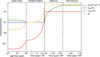 |
Fig. 2 Adopted physical condition in the hot core model. |
5.1 Photodissociation regions
Not many metal-bearing molecules have been found in PDRs because high UV radiation prevents the formation of stable molecular bonds. Any metal-bearing molecules that do form are quickly broken apart by UV photons. Table B.1 summarizes the abundances from our PDR model, including only those with abundances greater than 10−14 relative to hydrogen nuclei.
5.1.1 Metal-bearing species in PDRs: Detection attempts and model predictions
Schilke et al. (2001b) utilized the IRAM 30 m telescope to observe SiO transitions in PDRs such as the Orion Bar and S 140. SiO was detected with abundances around 10−11 relative to H2. Moreover, they also put limits of (2-4) × 10−11 toward several positions in NGC 2023 and NGC 7023. The findings suggest that while silicon is heavily depleted onto dust grains, a fraction returns to the gas phase near ionization fronts, possibly due to UV-driven processes or mild shocks. Our PDR model finds an abundance of 3.0 × 10⁻¹² relative to H2.
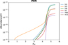 |
Fig. 3 Abundances of some notable metal-bearing species in the PDRs. |
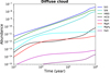 |
Fig. 4 Time evolution of abundances of some notable metal-bearing species in the diffuse clouds (nH = 50 cm−3). |
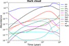 |
Fig. 5 Time evolution of abundances of some notable metal-bearing species in the dark clouds. |
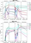 |
Fig. 6 Time evolution of abundances of some notable metal-bearing species in the hot cores. |
5.1.2 Other noteworthy species in PDRs
Table B.1 indicates that among the metal-bearing molecules, only some silicon-containing species are abundant in PDRs, with abundances exceeding 10−12. Specifically, SiH and SiC have abundances of approximately 10−11, while HCSi is roughly 10−12 relative to hydrogen. Moreover, as is highlighted in Table 2, it is noteworthy that both SiH and HCSi exhibit very weak dipole moments. This characteristic presents certain challenges when attempting to observe them through pure rotational transitions in PDRs.
5.2 Diffuse clouds
As with the PDRs, a limited number of metal-bearing molecules have been reported in the diffuse region due to the low densities and intense UV radiation. However, some attempts were made to estimate the upper limits for metal-bearing molecules in diffuse clouds.
5.2.1 Metal-bearing species in diffuse clouds: Detection attempts and model predictions
Czarny et al. (1987) searched for NaH and MgH in diffuse clouds using UV absorption spectroscopy but did not detect either molecule. They set upper limits for NaH and MgH with column densities of NaH ≤ 1.3 × 1010 cm−2 and MgH ≤ 1.9 × 109 cm−2 along the sightline to ζ Ophiuchi. NaH and MgH in our network primarily formed by grain surface reactions (Nagr + Hgr → NaHgr, Mggr + Hgr → MgHgr). NaH has a large dipole moment; however, based on our model, its abundance is approximately ~10−14−10−13, which suggests it is likely not observable. For MgH, we observed that our estimated abundance falls within the range of approximately 10−12 to 10−10, indicating that it may be within the detectable limits.
Lucas & Liszt (2000) estimated a SiO abundance of (2-20) × 10−11 for diffuse and translucent clouds that lie toward the extragalactic continuum sources. One transition of FeO was identified toward the ultracompact (UC) HII region associated with SgrB2(M) in absorption (Walmsley et al. 2002; Furuya et al. 2003). Walmsley et al. (2002) derived an abundance ratio of ~0.002 for FeO/SiO with FeO abundance of ~3 × 10⁻¹¹ with respect to H2. They estimated that the density of the absorbing gas is at a relatively low density and high temperature (−500 K). They suggested that the lower abundance of FeO would indicate that iron may be liberated by shocks, but it has yet to be processed in molecular form. Schilke et al. (2003) reported the detection of SiN having a very high abundance ~10−7 relative to H nuclei toward SgrB2(M) in absorption. Moreover, Schilke et al. (1997) estimated that 10% of the Si would be released by the shock and could contribute to the Si-related chemistry in the gas phase. They estimated a low density of nH2 = 103 cm−3 and a high temperature of ~500 K in the cloud, which may explain this feature. Compared to SiO, Schilke et al. (2003) estimated that the column density of SiN is 20-30 times lower.
While our diffuse cloud model may not be directly applicable under these conditions, it is still valuable to compare the abundances of FeO, SiN, and SiO derived from our model. Notably, as shown in Table B.2, we found FeO/SiO and SiO/SiN ratios of 0.001 and 10, respectively, for a hydrogen density (nH) of 500 cm−3. The table illustrates that we observed a significantly increased abundance of FeO when additional pathways were considered. In this case, the formation of FeO is primarily driven by gas-phase reactions, particularly through the exothermic reaction: FeH + O → FeO + H.
5.2.2 Other noteworthy species in diffuse clouds
Among the other silicate-bearing species, our study indicates that HNSi, SiC, and HCSi are abundant in diffuse clouds. Like SiN, the formation of HNSi appears through the dissociative recombination of SiNH2+ . Its formation is also significant by N + SiH2 → HNSi + H and N + SiH3 → HNSi + H2. HNSi can react with the major ions like H3+, H3O+, and HCO+ to produce SiNH2+. SiN is destroyed by oxygen (SiN + O), which does not apply to HNSi, possibly explaining why HNSi abundance is higher than that of SiN in our model. Interestingly, HNSi has not yet been detected in any astronomical observations. Parisel & Talbi (2000) attributed this discrepancy to the weak dipole moment of HNSi (0.25 Debye, see Table 2) or the possibility that dissociative recombination of SiNH2+ might not produce HNSi. HCSi has not yet been detected in space. Our diffuse cloud model, predicts a high abundance of HCSi and SiC. As indicated in Table 2, HCSi exhibits a modest dipole moment of 0.07 Debye. This small value could potentially account for its current challenges in detection.
Our model indicates a significant abundance of MgH2 at approximately 10−11−10−9. Despite having such a high abundance, its non-detection in the diffuse region may be attributed to its low dipole moment (0.18 Debye, see Table 2). Table B.2 illustrates an abnormally high abundance (on the order of a few times 10−7−10−5 of MgC2, MgC2H, MgC6H, and MgC8H in our diffuse cloud with nH =500 cm−3). However, with nH = 50 cm−3, we obtained a negligible abundance of these species. With the nH = 500 cm−3, the formation of MgC2, MgC2H, MgC6H, and MgC8H can be processed through a series of dissociative recombination reactions: MgCxH+ + e− → MgCxH/MgC2 + CyH/CyH2 (x=2,4, 6, 8 and y = 0, 2, 4, 6). The formation of MgC2 is also significantly influenced by the dissociative recombination of MgC2H+. During the initial phase, C2H2 is abundant; however, over time, larger hydrocarbons such as C6H2 and C8H2 become more prevalent compared to smaller hydrocarbons like C2H2 and C4H2. The primary production of MgC2, MgC2H, MgC6H, MgC8H mainly results from larger hydrocarbons, specifically MgC8H2+ and MgC6H2+. These larger hydrocarbons associate with Mg+ more quickly than the smaller ones, leading to an increased formation of MgC8H2+ and MgC6H2+ compared to MgC2H2+ and MgC4H2+.
5.3 Dark clouds
Metal-bearing molecules are rarely observed in dark clouds because metals are largely depleted onto dust grains, and the cold, dense conditions inhibit their desorption into the gas phase. Additionally, the emission lines of these molecules are often too weak to be detected with current sensitivity limits. However, several attempts have been made over the last few decades to observe these species in this region and estimate their abundances or the upper limits of observation.
5.3.1 Metal-bearing species in dark clouds: Detection attempts and model predictions
Turner et al. (2005) conducted a sensitive search for MgNC and AlNC in dark cloud core, TMC-1, with the Green Bank Telescope, and reported an upper limit of 1.2 × 10⁻¹¹ for MgNC. We did not consider the formation of AlNC in our network. Our dark cloud model with new pathways obtained a negligible abundance (−10−14) of MgNC. We have seen a significant impact on the MgNC abundance when its destruction by H, O, and C2H as suggested by Turner et al. (2005) is considered.
Ziurys et al. (1989); Ziurys (1991) estimated an upper limit for SiO and SiS abundance to be < 2.4 × 10⁻¹² and < 5.9 × 10⁻¹¹, respectively, in the TMC-1. Our dark cloud model obtained a SiO and SiS abundance of 3.6 × 10⁻⁹ and 2.6 × 10⁻¹², respectively. The abundance of SiO we obtained is notably higher than the upper limit established by Ziurys et al. (1989). It is to be noted that the new pathways have minimal impact on Si-bearing species. Thus, such a high SiO abundance was also obtained with the UMIST-2022 network as well.
Recently, several metal-bearing species have been identified in the quiescent molecular cloud G+0.693-0.27, located at the Central Molecular Zone of the Milky Way, or at least their upper abundance limits have been estimated (Massalkhi et al. 2023; Rey-Montejo et al. 2024). Our dark cloud model is more applicable for a source like TMC-1, which is cold (around 10 K) and well shielded. This environment facilitates slow chemical processes dominated by grain surfaces. In contrast, G+0.693-0.027 is warmer (approximately 50-100 K) and subject to comparatively intense radiation and shocks, which results in active gas-phase chemistry.
5.3.2 Other noteworthy species in dark clouds
Recently, the detection of rotational lines of AlF (ν = 0, J = 7-6) toward the S-type AGB star W Aql is reported by Danilovich et al. (2021). The first identification of AlF in M-type AGB stars is also reported by Saberi et al. (2022). However, AlF has not yet been identified in the dark cloud environment. The formation of AlF is included in the UMIST-2022 database. Table A.1 (available on Zenodo) presents some newly accounted ion-neutral destruction reactions for AlF. Without these additional pathways, the calculated abundance of AlF is 2.7 × 10⁻¹⁰, raising questions about why it has not been detected in the dark cloud. When considering newly accounted reactions, its abundance significantly drops to 1.4 × 10⁻¹³, a level that could explain its non-detection.
SiH4 is a non-polar spherical top molecule with a negligible rotationally induced dipole moment. Goldhaber & Betz (1984) identified Silane by its rotation-vibration spectrum. The pure rotational transitions of SiH4 would be extremely weak in the radio domain. Kolomiitsova et al. (2015) study the IR absorption spectra of SiH4 at 11 K. With the nitrogen matrix, they obtained a triplet in the stretching (2206.4 cm−1, 2203.0 cm−1, and 2196.5 cm−1) and a doublet in the bending region (910.3 cm−1 and 910.2 cm−1). Our modeling results suggest that in the dark cloud region, we have ample production of SiH4 in the ice phase. Tennyson et al. (2016; ExoMol) show that SiH4 has its largest cross section in the mid-IR ~4.5 μm, which could be accessible with the NIRSpec and PRISM instrument on board the James Webb Space Telescope (JWST). The bending doublet ~10.98 μm could also fall under the accessibility of JWST. A search for SiH3 has been carried out at the mid-IR domain by Cernicharo et al. (2017), but it was unsuccessful.
According to our dark-cloud model, the abundance of SiCH2 was estimated to be 1.1 × 10⁻¹¹. SiCH2 has not yet been detected in space, primarily due to its low dipole moment (0.18 Debye, see Table 2), which makes it challenging to identify in the gas phase. We obtained a significant abundance (9.4 × 10⁻¹²) of MgH2 from our dark cloud model. However, MgH2 has a linear, symmetric structure with a zero permanent dipole moment, preventing it from emitting rotational transitions. As a result, it cannot be detected using radio astronomy techniques that rely on dipole-induced rotational spectra. The ice-phase abundance of SiCH2 and MgH2 is approximately ~1.1 × 10⁻¹⁰ and 7 × 10⁻⁹, respectively. Given these abundances, the JWST may have the capability to detect these compounds through their IR vibrational transitions, which could provide valuable insights into their presence in various astrophysical environments.
5.4 Hot cores
Some metal-bearing molecules are detected in hot cores, as high temperatures and shocks may release metals from dust into the gas phase, enabling complex metal chemistry.
5.4.1 Metal-bearing species in Hot cores: Detection attempts and model predictions
SiO is ubiquitous in space. Generally, it is a good indicator of a shocked region. It is one of the first molecules discovered with radio astronomy (Wilson et al. 1971). Ziurys (1991) estimated a SiO abundance of ~1.2 × 10⁻⁹ in Orion KL. Our hot core model achieved a peak abundance of SiO ~3.4 × 10⁻¹⁰ during the warm-up and post-warm-up stages. Schilke et al. (2001a) tentatively identified SiH in Orion KL having fractional abundance of ~3 × 10⁻⁹. However, our hot core model underproduced SiH, having a peak gas-phase abundance of 7.2 × 10⁻¹². The observed underproduction of SiH and SiO in our model might be associated with the absence of shocks in the hot core model.
Turner (1991) estimated an upper limit of 1.6 × 10⁻⁹ for NaO in Orion KL. UMIST-2022 network did not consider the formation of NaO. The new pathways included in our network depict a peak gas-phase abundance of 5.4 × 10⁻¹¹ for NaO during the warm-up and post-warm-up stage of our hot core model. NaO in our model is mainly formed by the exothermic (having exothermicity of 8632 K) reaction: NaH + O → NaO + H.
Recently, NaCl has been detected in a massive protostellar system (Ginsburg et al. 2019; Wright et al. 2020). Our calculated binding energy indicates a high binding energy for NaCl (i.e., 15 019 K; see Table 1). Interestingly, our hot core model obtains a reasonable abundance of NaCl (having a peak abundance of 2.6 × 10⁻¹¹). The formation of NaCl in our hot core model results from the surface reaction between NaH and Cl during the warmup stage.
5.4.2 Other noteworthy species in hot cores
Though NaH has a significant dipole moment, it is yet to be identified in the hot core region because the warm and dense areas serve as sources for the local continuum, necessitating excitation above the background continuum to observe them in the submillimeter regime (Bernath et al. 1985). In our hot core model, we observed a favorable formation of NaH and MgH. In the cold phase, the formation of these compounds was primarily driven by pathways on grain surfaces. However, during the warmup and post-warm-up stages, the dissociative recombination of NaH2+ and MgH2+ plays a significant role. Additionally, certain exothermic channels of the reaction M1+ + M2 H → M1H + M2+ also make notable contributions to this process. Among the other hydrogen-bearing metals in hot cores, we have a notable abundance of MgH2 (peak abundance ~4.4 × 10⁻¹⁰) and FeH (~9.5 × 10⁻¹⁰).
Like diffuse and dark clouds, HNSi also appears to be abundant in hot cores, with an estimated abundance of approximately ~10−10. Among the carbon-bearing magnesium compounds, MgC2 and MgC2H are found to be present at abundances of 4.3 × 10⁻¹¹ and 1.9 × 10⁻¹², respectively. The formation of MgC2 in these phases was primarily driven by the dissociative recombination reaction of MgC2H+. Additionally, the formation of MgC2 H was mainly influenced by the dissociative recombination of MgCnH2+, where n can be 2, 6, or 8.
Table B.4 shows a significant increase in the abundance of FeO (~10−12) compared to when only the UMIST-2022 network was used. Additionally, we found that other notable species, such as AlO and AlF, are also abundant. The primary formation pathway identified for AlF was dominated by gas-phase reactions HF + Al → AlF + H and AlO + HF → AlF + OH. It is important to note that the abundance of AlO and FeO declines steadily after achieving a peak around 80 - 90 K. During the warm-up stage, another oxygen-bearing species, likely NaOH, maintains a steady abundance of approximately 10−10, making it an important species for future studies. Its formation in warm-up and post-warm-up stages is primarily influenced by the dissociative recombination of NaH2O+.
6 Conclusions
We used various state-of-the-art modeling to explore the fate of metal-bearing species in some astrophysical environments. Our calculations with a comprehensive reaction network containing the metal-related species suggest revisiting many unsuccessful searches conducted in the 1970s and 1980s. In the following, we highlight the main results:
The ionization process of a molecular cloud heavily relies on the depletion of metals, and it is crucial to have a realistic estimate of their binding energies. Quantum chemical calculations can be employed as a reliable alternative to laboratory measurements to make this estimation (Sil et al. 2024b). In dense media, water ice would be the most abundant surface species. In this study, we estimated the binding energy of some metals and their related species by considering water ice as the substrate. Based on their obtained binding energy values, they follow Fe, Si, Al, Na, K, and Mg in descending order. We used the water substrate to provide the binding energy for several metallic species, which can benefit astrochemical modeling. We found that the binding energies of some of the studied metals were significantly different from those used in earlier studies. For instance, we obtained much lower binding energies for Na and Mg (2408 K and 860 K, respectively), which were five to six times lower than the earlier estimations. However, the obtained binding energy (16 677 K) of Fe is about five times higher than previously known values. Our calculated binding energy for Si (7187 K) is consistent with the previously available calculations. Binding energy values forK and Al were not available, so we calculated them for the first time and obtained 2133 K and 4381 K, respectively. Another noteworthy aspect is the binding energy obtained for SiH4 (842 K), which is comparatively lower than that used in the past. We notice that MgNC, KH, and KCl favor chemisorption with the water surface, causing a change in molecular geometry;
Ion-molecular reactions play a crucial role in interstellar environments, occurring efficiently even at low temperatures and densities, significantly affecting the chemical composition of the ISM. The dipole moments of some of the metallic species considered here were unavailable; therefore, quantum chemical calculations were employed to ascertain the dipole moments for these species (see Table 2), which were subsequently integrated into the chemical model;
A list of gas-phase reactions, as presented in Table A.1 (available on Zenodo), was examined. The reaction enthalpies for several of these reactions were calculated using quantum chemical methods. Only those reactions that demonstrated exothermicity were incorporated into our network;
We made a significant effort to compile a list of reactions that should be included in astrochemical models, particularly when dealing with molecular clouds. During our study, we found important sets of reactions that could affect model abundance estimation:
- a)
One such notable reaction is M+ + H2 → MH2+ + hv, where M=Na, Fe, Mg, Al, Si, and K, which could trigger the formation of MH2+ and related chemistry. Usually, M=Si is considered in the network, but the others are neglected;
- b)
The reaction, MH + O → MO + H (M=Na, Mg, Al, and Fe), proposed by Turner (1991) is very important in dense regions for the production of metallic oxides;
- c)
M+1 + M2H → M1H + M+2 (where M1 ≠ M2, M1, M2 = Na, Mg, Si, Al, K, Fe) is also found to be important.
- a)
The destruction of MgNC by H, O, and C2H was proposed by Turner et al. (2005). In this study, we also considered similar destruction of MgCN, HMgNC, and MgC3N, but only if their reaction enthalpy is exothermic (see Table A.1, available on Zenodo). It is observed that the inclusion of these destruction processes has a significant impact on the abundances of these species;
In our study of the dense region, we observed that a significant amount of silicon gets trapped in the ice phase as SiH4. Our findings indicate that SiH4 has a much lower binding energy (842 K), so it may be released in the gas phase at significantly lower temperatures than previously assumed (~4500 K according to the OSU database). According to our hot core model, we could have a peak gas-phase SiH4 abundance of approximately 7.7 × 10⁻¹¹, and we also found that SiH3 is abundant from our hot core model (peak gas-phase abundance ~4.8 × 10⁻¹¹). SiH4 exhibits an intense bending feature in the IR spectrum around 11 μm (at 910.3 cm−1 and 910.2 cm−1) and has a large cross section at 4.5 μm that falls within the range of JWST. Our dark cloud model indicates that SiH4, MgH2, and SiCH2 are significantly abundant (approximately 10−10 to 10−9) relative to H2 in the ice phase, making them potentially observable species in cold dark molecular clouds for future identification with JWST;
It has been observed that HNSi and HCSi are present in detectable quantities in all the regions we studied. Additionally, the concentration of HNSi in UV radiation-shielded areas (such as diffuse, dark, and hot cores) is higher than that of SiN. However, while SiN has been identified, HNSi has not yet been detected. Our quantum chemical calculations, as noted in Table 2, indicate that both species possess a negligible dipole moment, which may explain their non-detection in the gas phase;
Ginsburg et al. (2019) propose that NaCl could form through the reaction between ionized sodium and HCl. However, we found that this reaction is highly endothermic and would not be feasible under the conditions in a hot core. In our study, the formation of NaCl is primarily driven by the surface reaction between NaH and Cl during the initial warming phase. We also found a relatively high abundance of NaOH, approximately 10−10, in our hot core model. Given its large dipole moment of about 6.7 Debye (as shown in Table 2), NaOH could be a promising candidate for future studies;
We identified a significant abundance of AlF in our dark cloud and hot core model through the UMIST network. However, it has not yet been observed in the regions studied here. The incorporation of ion-neutral destruction pathways significantly decreases its abundance.
Acknowledgements
A.D. acknowledges the Max Planck Society for sponsoring a scientific visit. Part of the Gaussian computations presented in this paper were performed using the GRICAD infrastructure (https://gricad.univ-grenoble-alpes.fr), supported by Grenoble research communities. M.S. acknowledges financial support from the European Research Council (consolidated grant COLLEXISM, grant agreement ID: 811363). P.C. acknowledges the support of the Max Planck Society. The authors thank Arghyadeb Roy for performing part of the Gaussian computations. The authors are thankful to the anonymous referee for the constructive comments and suggestions, which have significantly contributed to the revision of the paper.
Data availability
The data underlying this article (in the appendix) are made available under a Creative Commons Attribution license on Zenodo: doi: 10.5281/zenodo.15727282.
Appendix A Chemical reaction networks of metallic species with corresponding rate coefficients and enthalpies of formation for the species considered in this work.
Table A.1. Data underlying this table are made available under a Creative Commons Attribution license on Zenodo: doi: 10.5281/zenodo.15727282.
Enthalpies of formation for the species considered in this work.
Appendix B Abundance set
Abundances of relevant metallic species (> 10−14) in the PDR are presented for AV = 5.5 relative to total hydrogen nuclei.
Final abundances (after 106 years with respect to H2) of the metallic species for diffuse clouds (nH = 50 cm−3 and nH = 500 cm−3) having abundance > 10−12.
Final abundances (after 106 years relative to H2) of metallic species in dark clouds, exhibiting either abundances greater than 10−12 or targeted upper limits available.
Peak abundances (in between the warm-up and post-warm-up stage with respect to H2) of the metallic species for a hot core having abundance > 10−12.
References
- Abel, N. P., Ferland, G. J., Shaw, G., & van Hoof, P. A. M. 2005, ApJS, 161, 65 [NASA ADS] [CrossRef] [Google Scholar]
- Agúndez, M., & Wakelam, V. 2013, Chem. Rev., 113, 8710 [Google Scholar]
- Aikawa, Y., Miyama, S. M., Nakano, T., & Umebayashi, T. 1996, ApJ, 467, 684 [NASA ADS] [CrossRef] [Google Scholar]
- Asplund, M., Grevesse, N., Sauval, A. J., & Scott, P. 2009, ARA&A, 47, 481 [NASA ADS] [CrossRef] [Google Scholar]
- Baldwin, J. A., Ferland, G. J., Martin, P. G., et al. 1991, ApJ, 374, 580 [Google Scholar]
- Baldwin, J. A., Crotts, A., Dufour, R. J., et al. 1996, ApJ, 468, L115 [NASA ADS] [CrossRef] [Google Scholar]
- Belloche, A., Garrod, R. T., Müller, H. S. P., & Menten, K. M. 2014, Science, 345, 1584 [Google Scholar]
- Bernath, P. F., Black, J. H., & Brault, J. W. 1985, ApJ, 298, 375 [Google Scholar]
- Bhat, B., Gorai, P., Mondal, S. K., Chakrabarti, S. K., & Das, A. 2022, Adv. Space Res., 69, 415 [NASA ADS] [CrossRef] [Google Scholar]
- Cabezas, C., Cernicharo, J., Alonso, J. L., et al. 2013, ApJ, 775, 133 [NASA ADS] [CrossRef] [Google Scholar]
- Cernicharo, J. 2012, in EAS Publications Series, 58, eds. C. Stehlé, C. Joblin, & L. d’Hendecourt, 251 [Google Scholar]
- Cernicharo, J., & Guelin, M. 1987, A&A, 183, L10 [Google Scholar]
- Cernicharo, J., Agúndez, M., Velilla Prieto, L., et al. 2017, A&A, 606, L5 [NASA ADS] [CrossRef] [EDP Sciences] [Google Scholar]
- Cernicharo, J., Cabezas, C., Pardo, J. R., et al. 2019a, A&A, 630, L2 [NASA ADS] [CrossRef] [EDP Sciences] [Google Scholar]
- Cernicharo, J., Velilla-Prieto, L., Agúndez, M., et al. 2019b, A&A, 627, L4 [NASA ADS] [CrossRef] [EDP Sciences] [Google Scholar]
- Chantzos, J., Rivilla, V. M., Vasyunin, A., et al. 2020, A&A, 633, A54 [NASA ADS] [CrossRef] [EDP Sciences] [Google Scholar]
- Curtiss, L. A., Raghavachari, K., Redfern, P. C., & Pople, J. A. 1997, J. Chem. Phys., 106, 1063 [Google Scholar]
- Czarny, J., Felenbok, P., & Roueff, E. 1987, A&A, 188, 155 [Google Scholar]
- Danilovich, T., Van de Sande, M., Plane, J. M. C., et al. 2021, A&A, 655, A80 [NASA ADS] [CrossRef] [EDP Sciences] [Google Scholar]
- Das, A., Majumdar, L., Sahu, D., et al. 2015, ApJ, 808, 21 [NASA ADS] [CrossRef] [Google Scholar]
- Das, A., Sil, M., Gorai, P., Chakrabarti, S. i. K., & Loison, J. C. 2018, ApJs, 237, 9 [Google Scholar]
- Das, A., Gorai, P., & Chakrabarti, S. K. 2019, A&A, 628, A73 [NASA ADS] [CrossRef] [EDP Sciences] [Google Scholar]
- Das, A., Sil, M., Bhat, B., et al. 2020, ApJ, 902, 131 [Google Scholar]
- Das, A., Sil, M., Ghosh, R., et al. 2021, Front. Astron. Space Sci., 8 [Google Scholar]
- Dunning, Thom H. J. 1989, J. Chem. Phys., 90, 1007 [NASA ADS] [CrossRef] [Google Scholar]
- Ferland, G. J., Chatzikos, M., Guzmán, F., et al. 2017, RMxAA, 53, 385 [NASA ADS] [Google Scholar]
- Frisch, M. J., Trucks, G. W., Schlegel, H. B., et al. 2016, Gaussian 16 Revision B.01 (Wallingford, CT: Gaussian Inc.) [Google Scholar]
- Furuya, R. S., Walmsley, C. M., Nakanishi, K., Schilke, P., & Bachiller, R. 2003, A&A, 409, L21 [NASA ADS] [CrossRef] [EDP Sciences] [Google Scholar]
- Garrod, R. T., & Pauly, T. 2011, ApJ, 735, 15 [Google Scholar]
- Garrod, R. T., Wakelam, V., & Herbst, E. 2007, A&A, 467, 1103 [NASA ADS] [CrossRef] [EDP Sciences] [Google Scholar]
- Garrod, R. T., Belloche, A., Müller, H. S. P., & Menten, K. M. 2017, A&A, 601, A48 [NASA ADS] [CrossRef] [EDP Sciences] [Google Scholar]
- Ghosh, R., Sil, M., Kumar Mondal, S., et al. 2022, Res. Astron. Astrophys., 22, 065021 [CrossRef] [Google Scholar]
- Ginsburg, A., McGuire, B., Plambeck, R., et al. 2019, ApJ, 872, 54 [NASA ADS] [CrossRef] [Google Scholar]
- Goldhaber, D. M., & Betz, A. L. 1984, ApJ, 279, L55 [NASA ADS] [CrossRef] [Google Scholar]
- Gorai, P., Das, A., Das, A., et al. 2017, ApJ, 836, 70 [Google Scholar]
- Gorai, P., Bhat, B., Sil, M., et al. 2020, ApJ, 895, 86 [Google Scholar]
- Guelin, M., Lucas, R., & Cernicharo, J. 1993, A&A, 280, L19 [Google Scholar]
- Guélin, M., Muller, S., Cernicharo, J., et al. 2000, A&A, 363, L9 [NASA ADS] [Google Scholar]
- Guélin, M., Muller, S., Cernicharo, J., McCarthy, M. C., & Thaddeus, P. 2004, A&A, 426, L49 [NASA ADS] [CrossRef] [EDP Sciences] [Google Scholar]
- Hasegawa, T. I., & Herbst, E. 1993, MNRAS, 261, 83 [NASA ADS] [CrossRef] [Google Scholar]
- Herbst, E., & Klemperer, W. 1973, ApJ, 185, 505 [Google Scholar]
- Highberger, J. L., Thomson, K. J., Young, P. A., Arnett, D., & Ziurys, L. M. 2003, ApJ, 593, 393 [NASA ADS] [CrossRef] [Google Scholar]
- Hollenbach, D. J., & Tielens, A. G. G. M. 1997, ARA&A, 35, 179 [NASA ADS] [CrossRef] [Google Scholar]
- Indriolo, N., Neufeld, D. A., Gerin, M., et al. 2012, ApJ, 758, 83 [NASA ADS] [CrossRef] [Google Scholar]
- Kolomiitsova, T. D., Savvateev, K. F., Shchepkin, D. N., Tokhadze, I. K., & Tokhadze, K. G. 2015, J. Phys. Chem. A, 119, 2553 [Google Scholar]
- Lucas, R., & Liszt, H. S. 2000, A&A, 355, 327 [NASA ADS] [Google Scholar]
- Massalkhi, S., Jiménez-Serra, I., Martin-Pintado, J., et al. 2023, A&A, 678, A45 [NASA ADS] [CrossRef] [EDP Sciences] [Google Scholar]
- Mathis, J. S., Rumpl, W., & Nordsieck, K. H. 1977, ApJ, 217, 425 [Google Scholar]
- McElroy, D., Walsh, C., Markwick, A. J., et al. 2013, A&A, 550, A36 [NASA ADS] [CrossRef] [EDP Sciences] [Google Scholar]
- Merer, A. J., Walmsley, C. M., & Churchwell, E. 1982, ApJ, 256, 151 [Google Scholar]
- Millar, T. J., Walsh, C., Van de Sande, M., & Markwick, A. J. 2024, A&A, 682, A109 [NASA ADS] [CrossRef] [EDP Sciences] [Google Scholar]
- Mondal, S. K., Gorai, P., Sil, M., et al. 2021, ApJ, 922, 194 [NASA ADS] [CrossRef] [Google Scholar]
- Muñoz Caro, G. M., Jiménez-Escobar, A., Martín-Gago, J. A., et al. 2010, A&A, 522, A108 [NASA ADS] [CrossRef] [EDP Sciences] [Google Scholar]
- Neufeld, D. A., Welty, D. E., Ivlev, A. V., et al. 2024, ApJ, 973, 143 [Google Scholar]
- Öberg, K. I., Fuchs, G. W., Awad, Z., et al. 2007, ApJ, 662, L23 [Google Scholar]
- Öberg, K. I., Garrod, R. T., van Dishoeck, E. F., & Linnartz, H. 2009, A&A, 504, 891 [NASA ADS] [CrossRef] [EDP Sciences] [Google Scholar]
- Obolentseva, M., Ivlev, A. V., Silsbee, K., et al. 2024, ApJ, 973, 142 [NASA ADS] [CrossRef] [Google Scholar]
- Osterbrock, D. E., Tran, H. D., & Veilleux, S. 1992, ApJ, 389, 305 [Google Scholar]
- Parisel, O., & Talbi, D. 2000, Quantum Molecular Systems in Astrophysics: the Illustrative Example of Interstellar Nitriles and Silanitriles, eds. A. Hernández-Laguna, J. Maruani, R. McWeeny, & S. Wilson (Dordrecht: Springer Netherlands), 261 [Google Scholar]
- Penteado, E. M., Walsh, C., & Cuppen, H. M. 2017, ApJ, 844, 71 [Google Scholar]
- Pulliam, R. L., Savage, C., Agúndez, M., et al. 2010, ApJ, 725, L181 [NASA ADS] [CrossRef] [Google Scholar]
- Ramachandran, R., Sil, M., Gorai, P., et al. 2024, ApJ, 975, 181 [Google Scholar]
- Rawlings, J. M. C., Hartquist, T. W., Menten, K. M., & Williams, D. A. 1992, MNRAS, 255, 471 [CrossRef] [Google Scholar]
- Rey-Montejo, M., Jiménez-Serra, I., Martín-Pintado, J., et al. 2024, ApJ, 975, 174 [NASA ADS] [CrossRef] [Google Scholar]
- Ruaud, M., Wakelam, V., & Hersant, F. 2016, MNRAS, 459, 3756 [Google Scholar]
- Rubin, R. H., Dufour, R. J., & Walter, D. K. 1993, ApJ, 413, 242 [Google Scholar]
- Saberi, M., Khouri, T., Velilla-Prieto, L., et al. 2022, A&A, 663, A54 [NASA ADS] [CrossRef] [EDP Sciences] [Google Scholar]
- Schilke, P., Walmsley, C. M., Pineau des Forets, G., & Flower, D. R. 1997, A&A, 321, 293 [NASA ADS] [Google Scholar]
- Schilke, P., Benford, D. J., Hunter, T. R., Lis, D. C., & Phillips, T. G. 2001a, ApJS, 132, 281 [Google Scholar]
- Schilke, P., Pineau des Forêts, G., Walmsley, C. M., & Martín-Pintado, J. 2001b, A&A, 372, 291 [NASA ADS] [CrossRef] [EDP Sciences] [Google Scholar]
- Schilke, P., Leurini, S., Menten, K. M., & Alcolea, J. 2003, A&A, 412, L15 [NASA ADS] [CrossRef] [EDP Sciences] [Google Scholar]
- Shaw, G., Ferland, G. J., & Chatzikos, M. 2022, ApJ, 934, 53 [NASA ADS] [CrossRef] [Google Scholar]
- Sil, M., Gorai, P., Das, A., Sahu, D., & Chakrabarti, S. K. 2017, Eur. Phys. J. D, 71, 45 [Google Scholar]
- Sil, M., Gorai, P., Das, A., et al. 2018, ApJ, 853, 139 [NASA ADS] [CrossRef] [Google Scholar]
- Sil, M., Srivastav, S., Bhat, B., et al. 2021, AJ, 162, 119 [NASA ADS] [CrossRef] [Google Scholar]
- Sil, M., Das, A., Das, R., et al. 2024a, A&A, 692, A264 [NASA ADS] [CrossRef] [EDP Sciences] [Google Scholar]
- Sil, M., Roy, A., Gorai, P., et al. 2024b, A&A, 690, A252 [NASA ADS] [CrossRef] [EDP Sciences] [Google Scholar]
- Sil, M., Faure, A., Wiesemeyer, H., et al. 2025, A&A, 695, A244 [NASA ADS] [CrossRef] [EDP Sciences] [Google Scholar]
- Srivastav, S., Sil, M., Gorai, P., et al. 2022, MNRAS, 515, 3524 [NASA ADS] [CrossRef] [Google Scholar]
- Su, T., & Chesnavich, W. J. 1982, J. Chem. Phys., 76, 5183 [NASA ADS] [CrossRef] [Google Scholar]
- Tanaka, K. E. I., Zhang, Y., Hirota, T., et al. 2020, ApJ, 900, L2 [NASA ADS] [CrossRef] [Google Scholar]
- Tennyson, J., Yurchenko, S. N., Al-Refaie, A. F., et al. 2016, J. Mol. Spectrosc., 327, 73 [Google Scholar]
- Turner, B. E. 1991, ApJ, 376, 573 [Google Scholar]
- Turner, B. E. 1992, in Astrochemistry of Cosmic Phenomena, eds. P. D. Singh (Dordrecht: Springer Netherlands), 181 [Google Scholar]
- Turner, B. E., Steimle, T. C., & Meerts, L. 1994, ApJ, 426, L97 [NASA ADS] [CrossRef] [Google Scholar]
- Turner, B. E., Petrie, S., Dunbar, R. C., & Langston, G. 2005, ApJ, 621, 817 [Google Scholar]
- Wakelam, V., Loison, J. C., Mereau, R., & Ruaud, M. 2017, Mol. Astrophys., 6, 22 [NASA ADS] [CrossRef] [Google Scholar]
- Walmsley, C. M., Bachiller, R., Pineau des Forêts, G., & Schilke, P. 2002, ApJ, 566, L109 [Google Scholar]
- Weigend, F., & Ahlrichs, R. 2005, Phys. Chem. Chem. Phys. (Incorp. Faraday Trans.), 7, 3297 [Google Scholar]
- Wilson, R. W., Penzias, A. A., Jefferts, K. B., Kutner, M., & Thaddeus, P. 1971, ApJ, 167, L97 [NASA ADS] [CrossRef] [Google Scholar]
- Wright, M., Plambeck, R., Hirota, T., et al. 2020, ApJ, 889, 155 [Google Scholar]
- Zack, L. N., Halfen, D. T., & Ziurys, L. M. 2011, ApJ, 733, L36 [NASA ADS] [CrossRef] [Google Scholar]
- Ziurys, L. M. 1991, ApJ, 379, 260 [NASA ADS] [CrossRef] [Google Scholar]
- Ziurys, L. M., Apponi, A. J., Guelin, M., & Cernicharo, J. 1995, ApJ, 445, L47 [NASA ADS] [CrossRef] [Google Scholar]
- Ziurys, L. M., Friberg, P., & Irvine, W. M. 1989, ApJ, 343, 201 [NASA ADS] [CrossRef] [Google Scholar]
- Ziurys, L. M., Savage, C., Highberger, J. L., et al. 2002, ApJ, 564, L45 [NASA ADS] [CrossRef] [Google Scholar]
- Zucconi, A., Walmsley, C. M., & Galli, D. 2001, A&A, 376, 650 [NASA ADS] [CrossRef] [EDP Sciences] [Google Scholar]
All Tables
Computed binding energies of metal-bearing species considering water monomer (default) as the substrate while incorporating a scaling factor of 1.416 (see text for details).
Initial elemental abundances considered for the H II-PDR, diffuse clud, dark cloud, and hot core cloud models with respect to total hydrogen nuclei.
Abundances of relevant metallic species (> 10−14) in the PDR are presented for AV = 5.5 relative to total hydrogen nuclei.
Final abundances (after 106 years with respect to H2) of the metallic species for diffuse clouds (nH = 50 cm−3 and nH = 500 cm−3) having abundance > 10−12.
Final abundances (after 106 years relative to H2) of metallic species in dark clouds, exhibiting either abundances greater than 10−12 or targeted upper limits available.
Peak abundances (in between the warm-up and post-warm-up stage with respect to H2) of the metallic species for a hot core having abundance > 10−12.
All Figures
|
Fig. 1 Upper panel: total hydrogen number density, electron number density, and temperature variation. Lower panel: abundance variation of various H, C, and O-related species with respect to total hydrogen nuclei in the HII to PDR obtained from the Cloudy code. |
| In the text | |
|
Fig. 2 Adopted physical condition in the hot core model. |
| In the text | |
|
Fig. 3 Abundances of some notable metal-bearing species in the PDRs. |
| In the text | |
|
Fig. 4 Time evolution of abundances of some notable metal-bearing species in the diffuse clouds (nH = 50 cm−3). |
| In the text | |
|
Fig. 5 Time evolution of abundances of some notable metal-bearing species in the dark clouds. |
| In the text | |
|
Fig. 6 Time evolution of abundances of some notable metal-bearing species in the hot cores. |
| In the text | |
Current usage metrics show cumulative count of Article Views (full-text article views including HTML views, PDF and ePub downloads, according to the available data) and Abstracts Views on Vision4Press platform.
Data correspond to usage on the plateform after 2015. The current usage metrics is available 48-96 hours after online publication and is updated daily on week days.
Initial download of the metrics may take a while.