| Issue |
A&A
Volume 700, August 2025
|
|
|---|---|---|
| Article Number | A68 | |
| Number of page(s) | 30 | |
| Section | Extragalactic astronomy | |
| DOI | https://doi.org/10.1051/0004-6361/202452406 | |
| Published online | 06 August 2025 | |
Quenching of galaxies at cosmic noon
Understanding the effect of the environment
1
European Southern Observatory, Alonso de Córdova 3107, Vitacura, Santiago de Chile, Chile
2
Universidad Andres Bello, Facultad de Ciencias Exactas, Departamento de Fisica, Instituto de Astrofisica, Fernandez Concha 700, Las Condes, Santiago RM, Chile
3
Department of Physics and Astronomy, Purdue University, 525 Northwestern Avenue, West Lafayette, IN 47907, USA
4
Instituto de Astronomía Teórica y Experimental (IATE), CONICET-UNC, Laprida 854, X500BGR Córdoba, Argentina
5
Department of Physics and Astronomy, Rutgers, the State University of New Jersey, Piscataway, NJ 08854, USA
6
Department of Astronomy and Space Science, Chungnam National University, 99 Daehak-ro, Yuseong-gu, Daejeon 34134, Republic of Korea
7
Department of Physics and Astronomy, Seoul National University, 1 Gwanak-ro, Gwanak-gu, Seoul 08826, Republic of Korea
8
SNU Astronomy Research Center, Seoul National University, 1 Gwanak-ro, Gwanak-gu, Seoul 08826, Republic of Korea
9
Universidad Central de Chile, Avenida Francisco de Aguirre 0405, 171-0614 La Serena, Coquimbo, Chile
10
Department of Astronomy and Astrophysics, The Pennsylvania State University, University Park, PA 16802, USA
11
Institute for Gravitation and the Cosmos, The Pennsylvania State University, University Park, PA 16802, USA
12
NSFs National Optical-Infrared Astronomy Research Laboratory, 950 N. Cherry Ave., Tucson AZ 85719, USA
13
Korea Institute for Advanced Study, 85 Hoegi-ro, Dongdaemun-gu, Seoul 02455, Republic of Korea
14
Korea Astronomy and Space Science Institute, 776 Daedeokdae-ro, Yuseong-gu, Daejeon 34055, Republic of Korea
15
Millennium Nucleus for Galaxies (MINGAL), Chile
⋆ Corresponding author: This email address is being protected from spambots. You need JavaScript enabled to view it.
Received:
29
September
2024
Accepted:
22
May
2025
Abstract
Context. We identified and analysed massive quiescent galaxies (MQGs) at z ≈ 3.1 within the 2 deg2 COSMOS field and explored the effect of the galaxy environment on quenching processes. By examining the variation in the quenched fraction and physical properties of these galaxies in different environmental contexts, including local densities, protoclusters, and cosmic filaments, we investigated the connection between environmental factors and galaxy quenching at cosmic noon.
Aims. We selected MQGs at z ≈ 3.1 using deep photometric data from the COSMOS2020 catalogue combined with narrow-band-selected Lyman-α emitters (LAEs) from the One-hundred-square-degree DECam Imaging in Narrowbands (ODIN) survey. We performed a spectral energy distribution fitting using the code BAGPIPES to derive the star formation histories and quenching timescales. We constructed Voronoi-tessellation density maps using LAEs, and we independently selected galaxies photometrically to characterize the galaxy environments.
Methods. We identified 24 MQGs at z ≈ 3.1, each of which has a stellar mass higher than 1010.6 M⊙. These MQGs share remarkably uniform star-formation histories, with intense starburst phases followed by rapid quenching within short timescales (≤400 Myr). The consistency of these quenching timescales suggests a universal and highly efficient quenching mechanism in this epoch. We found no significant correlation between environmental density (either local or large scale) and galaxy quenching parameters such as the quenching duration, the quenched fraction, or the timing. MQGs show no preferential distribution with respect to protoclusters or filaments compared to massive star-forming galaxies. Some MQGs reside close to gas-rich filaments, but show no evidence of rejuvenated star formation. This implies gas-heating mechanisms and not gas exhaustion. These results indicate that the quenching processes at z ≈ 3.1 likely depend little on the immediate galaxy environment.
Results. Our findings suggest that environmental processes alone, such as galaxy mergers, interactions, or gas stripping, cannot fully explain the galaxy quenching at z ≈ 3.1. Internal mechanisms such as feedback from AGN, stellar feedback, virial shock heating, or morphological quenching instead play an important role in quenching. Future spectroscopic observations must confirm the quiescent nature and precise redshifts of these galaxies. Observational studies of gas dynamics, gas temperature, and ionisation conditions within and around MQGs will also clarify the physical mechanisms driving galaxy quenching during this critical epoch of galaxy evolution.
Key words: galaxies: evolution / galaxies: high-redshift / large-scale structure of Universe / infrared: galaxies
© The Authors 2025
 Open Access article, published by EDP Sciences, under the terms of the Creative Commons Attribution License (https://creativecommons.org/licenses/by/4.0), which permits unrestricted use, distribution, and reproduction in any medium, provided the original work is properly cited.
This article is published in open access under the Subscribe to Open model. This email address is being protected from spambots. You need JavaScript enabled to view it. to support open access publication.
1. Introduction
Observations and simulations have shown a clear bi-modality in various properties of galaxies, such as their colours, morphologies, and star formation rates (SFRs) (Dressler 1980). Quiescent galaxies(QGs) are characterised by redder colours and typically a spheroidal morphology, whereas star-forming galaxies exhibit bluer colours and typically show a disk-like morphology. However, there is a gap in our understanding of the mechanisms that stop the star formation in bluer galaxies and quench them so that they become redder QGs.
Quenching mechanisms are generally categorised as mass quenching or environmental quenching (Peng et al. 2010). Mass quenching refers to internal processes that correlate with the stellar mass of a galaxy, such as stellar feedback and Active Galactic Nuclei (AGN) feedback(e.g. Croton et al. 2006; Ceverino & Klypin 2009; Fabian 2012; Cicone et al. 2014). Environmental quenching refers to external processes such as ram-pressure stripping (e.g. Gunn & Gott 1972), strangulation (Larson 1990), and galaxy harassment (Moore et al. 1996; Park & Hwang 2009), which depend on the environment in which the galaxy resides. Although both mass and environmental quenching affect the cessation of star formation, their relative importance depends on the mass of the galaxy and the cosmic epoch. In the local Universe, the relation between SFR and environment density is well established. According to this relation, quenched galaxies preferentially occur in dense environments, such as clusters. In contrast, star-forming galaxies predominantly exist in relatively low-density environments because in local virialised clusters, environmental processes can remove or heat cold gas from galaxies (Boselli & Gavazzi 2006). This accelerates quenching phenomena and increases the fraction of quenched galaxies.
In recent years, the existence of QGs at redshifts z ≈ 3–4 (e.g. Spitler et al. 2014; Straatman et al. 2014; Girelli et al. 2019; Carnall et al. 2018, 2023) has been corroborated by spectroscopic confirmations (e.g. Glazebrook et al. 2017, 2022; Schreiber et al. 2018; D’Eugenio et al. 2020; Nanayakkara et al. 2024). At lower redshift (z < 1), environmental quenching typically occurs on timescales of several billion years (Mao et al. 2022), but at z = 3, the Universe was only about two billion years old, and the quenching processes must have acted faster. This raises the question which processes quenched galaxies at z > 3. Some studies suggested that high-density environments promote star formation and are dominated by starburst galaxies(Casey 2016; Calvi et al. 2023), whereas other research found QGs in compact groups (Ito et al. 2023; Tanaka et al. 2024). We conducted a statistical analysis of QGs and their environments at z = 3.1 to determine whether the environment and the quenching are systemically related.
To trace the environmental density, we used two tracers: all the galaxies listed in the COSMOS2020 catalogue (Weaver et al. 2021), which were selected based on their photometric redshift (photo-z); and Lyman-α emitting galaxies (LAEs) from the One-hundred-square-degree DECam Imaging in Narrowbands (ODIN) survey (Lee et al. 2024). The first galaxy sample is meant not to be biased in terms of physical properties, while LAEs are characterised by a strong Lyman-α emission line. The Lyα emission line ( ) is the strongest recombination line of neutral hydrogen and has been used to trace star formation, AGN activity, and the gravitational collapse of dark matter haloes at redshift ≥2 (Ouchi et al. 2020). Given the wavelength of the Lyα emission, LAEs can be detected up to z ≈ 6 using ground-based photometric surveys, which makes them an ideal tool for tracing the underlying density distribution and the large-scale structure over wide areas (e.g. Hu & McMahon 1996; Ouchi et al. 2003; Gawiser et al. 2007; Kovač et al. 2007). With the photo-z selected galaxies and LAEs, we created two density maps that we used to study the environment of QGs.
Some studies based on simulations have suggested that AGN feedback is the primary quenching mechanism for high-redshift QGs (Kurinchi-Vendhan et al. 2024; Hartley et al. 2023). Kurinchi-Vendhan et al. (2024) found in the IllustrisTNG simulation that the number of merger events in a galaxy’s history is not sufficient to distinguish between quiescent and star-forming galaxies and that AGN feedback is required to quench the galaxy. By using the Magneticum simulation, Kimmig et al. (2025) showed that while AGN-driven gas removal quenches galaxies, quenching is also influenced by the environment. They found that for a galaxy to be quenched, it must reside in a significant underdensity that prevents the gas from being replenished. The aim of our study here is to observationally assess the extent of the environmental impact on galaxy quenching at z = 3.1.
To search for QGs, we made use of archival photometric data in the optical and near- and mid-IR bands. The data we used to select the galaxies and determine the density map criteria are given in Sections 2.1 and 2.2. The spectral energy distribution (SED) fitting analysis needed to determine the passive nature of QGs is described in Section 2.4. We describe the selection of QGs in Section 2.5. In Section 2.8 we describe the density maps we constructed using LAEs and photo-z selected galaxies. A summary of the results is presented in Section 3. A discussion of our results and a comparison with previous observations and current simulations is presented in Section 4. Throughout this paper, a standard cold dark matter cosmology is adopted with the Hubble constant H0 = 70 km s−1 Mpc−1, the total matter density ΩM = 0.3, and the dark energy density ΩΛ = 0.7. All magnitudes are expressed in the AB system, and log is the base 10 logarithm if not specified otherwise.
2. Data and methods
In this section, we describe the archival and the new observed data we employed to select galaxies at z ≈ 3.1. These galaxies were used to create density maps to trace the large-scale environment, as described in Sections 2.6, 2.7 and 2.8. We also describe the SED fitting method we used to identify QGs from the selected galaxies.
2.1. The One-hundred-deg2 DECam Imaging in Narrowbands Survey
The One-hundred-square-degree DECam Imaging in Narrowbands (ODIN) survey uses Lyman-alpha (Lyα) emitting galaxies to trace the cosmic structures and overdensities in the following redshift slices: z ≈ 4.5, 3.1, and 2.4 (tage = 1.3, 2.0, and 2.7 Gyr since the Big Bang). The adopted N419, N501, and N673 filters have central wavelengths of 419 nm, 501 nm, and 673 nm, respectively, which cover the Lyman-alpha line at the redshifts mentioned above and have full widths at half maximum (FWHM) of 7.5 nm, 7.6 nm, and 10.0 nm, respectively. The LAEs were selected as narrow-band excess compared to the existing broad-band data from Hyper-Suprime-Cam Subaru. ODIN aims to select more than 100 000 LAEs at the three cosmic epochs (Lee et al. 2024).
The ODIN survey reaches a 5σ sensitivity of 25.7 mag (N501 filter) at z ≈ 3.1, with a redshift precision of Δz = 0.062. The corresponding Lyman-α luminosity is LLyα ≈ 1.43 × 1042 erg s−1. The LAEs that are detected at z ≈ 3.1 have a median log(SFR/M⊙ yr−1) = 0.77 ± 0.2 and log(M/M⊙) = 8.8 ± 0.2, and a median dust attenuation of AV = 0.5 ± 0.1. The LAE number density at this redshift is 0.20 arcmin−2. The survey design and LAE selection in the ODIN survey are described in detail by Lee et al. (2024) and Firestone et al. (2024), respectively. We used the LAEs selected in the Cosmic Evolution Survey (COSMOS) field (Scoville et al. 2007) as described by Firestone et al. (2024). We concentrated on redshift ≈3.1 in the COSMOS field because the ODIN observations at this redshift (N501 filter) have been fully acquired and reduced, and the LAE density map has been published (Ramakrishnan et al. 2023).
2.2. Publicly available data
The COSMOS field is a 2-square-degrees field with the deepest available near-infrared wide-field coverage (Scoville et al. 2007; McCracken et al. 2012; Weaver et al. 2021; Dunlop et al. 2023). The COSMOS2020 photometric catalogue (Weaver et al. 2021), includes ultra-deep optical data from the Subaru Hyper-Suprime-Cam (Aihara et al. 2019), ultra-deep U-band CLAUDS data (Sawicki et al. 2019), ultra-deep near-infrared UltraVISTA data (Dunlop et al. 2023), and SpitzerIRAC data (Weaver et al. 2021). The deep Ultra-VISTA data and Spitzer data are well suited for a search of optically faint galaxies such as QGs. We used the COSMOS2020 catalogue, which was produced using a profile fitting photometry method (known as the COSMOS FARMER catalogue). The galaxies in COSMOS2020 were selected from a near-infrared izY JHKs CHI-MEAN co-added detection image. Of these bands, the i band is the most sensitive. It reaches a 3σ depth of approximately 27 mag. The Ks band is the shallowest band at a depth of about 25 mag 3σ. The Ks band plays a key role in selecting mass-complete samples up to z ≤ 4.5. Its increased depth (0.5–0.8 mag deeper than the COSMOS2015 catalogue) improves the completeness, in particular, for low-mass galaxies. Combined with IRAC data, these observation also enhance the detection of old, red, and dust-obscured sources. For the brightest galaxies (i < 22.5), the catalogue achieves a high redshift accuracy, with an outlier rate lower than 1%. Even for fainter sources in the 25 < i < 27 range, photometric redshift estimates maintain a precision of ≈4%, but with a higher outlier rate of ≈20%. The stellar mass completeness thresholds (defined as the redshift-dependent limits at which samples remain ≈70% complete) were established as listed below.
-
All galaxies: M⋆ = −3.23 × 10⁷(1 + z)+7.83 × 10⁷(1 + z)2
-
Star-forming galaxies: M⋆ = −5.77 × 10⁷(1 + z)+8.66 × 10⁷(1 + z)2
-
Quiescent galaxies: M⋆ = −3.79 × 10⁸(1 + z)+2.98 × 10⁸(1 + z)2
For further details of the photometry, SED fitting, mass function, and luminosity function, we refer to Weaver et al. (2021) and Weaver et al. (2023). We also used the photometric redshifts estimated from LePHARE (Arnouts et al. 1999) that are provided in the catalogue.
2.3. Selection of galaxies at redshift z ≈ 3.1
For the COSMOS2020 catalogue, Weaver et al. (2021) discussed the accuracy of photometric redshifts obtained using the code LePHARE (Arnouts et al. 1999) by comparing them to spectroscopic redshifts. They reported that the LePHARE photometric redshifts show a high degree of consistency with the spectroscopic redshifts in the COSMOS field and achieve a subpercent photometric redshift accuracy. The precision of photometric redshifts is approximately 0.01 × (1 + z) for galaxies with an i-band magnitude < 22.5. For fainter magnitudes, the precision decreases, but remains better than 0.025 × (1 + z) for i < 25. Based on this good quality of photo-z in the COSMOS2020 catalogue, we used the LePHARE photo-z to select the sample of galaxies at z ≈ 3.1.
We applied no additional mass cut to select galaxies from the COSMOS 2020 catalogue. Based on the relations in Section 2.2, at z = 3.1, the stellar mass completeness thresholds are
-
all galaxies: Mlim = 1.18 × 10⁹ M⊙
-
star-forming galaxies: Mlim = 1.22 × 10⁹ M⊙
-
quiescent galaxies: Mlim = 3.46 × 10⁹ M⊙.
To ensure a balance between sample completeness and purity, we adopted a redshift range of Δz = 0.12 centred at z = 3.1. We selected galaxies such that 68% of the redshift probability distribution function of our selected galaxies was confined to 3.004 ≤ zphot ≤ 3.16. With this criterion, we selected 6431 galaxies. This selection ensured a clean sample with a low uncertainty in the redshift range. To identify the QGs from this sample, we performed the SED fitting using the photometric data available in the COSMOS2020 catalogue.
2.4. SED fitting using BAGPIPES
The Python code called Bayesian Analysis of Galaxies for Physical Inference and Parameter EStimation (BAGPIPES, Carnall et al. 2018, 2023) models galaxy spectra and fits spectroscopic and photometric observations simultaneously. BAGPIPES has recently been used successfully to study QGs (see e.g. Jin et al. 2024). We used the code BAGPIPES to fit the COSMOS2020 SEDs of all 6431 z ≊ 3.1 galaxies and to estimate their specific star formation rate (sSFR).
We fitted the SED using all 29 photometric bands in the COSMOS2020 catalogue. We adopted a double power-law star formation history (SFH) model, which effectively captures the rising and declining phases of the SFH with two distinct power-law slopes. The functional form of the SFH is given by
![Mathematical equation: $$ \begin{aligned} \mathrm{SFR(t)} \propto \left[ \left( \frac{t}{\tau } \right)^\alpha + \left( \frac{t}{\tau } \right)^{-\beta } \right]^{-1} , \end{aligned} $$](/articles/aa/full_html/2025/08/aa52406-24/aa52406-24-eq2.gif) (1)
(1)
where α and β are the falling and rising slopes, respectively, and τ is related to the time at which the star formation peaks. Carnall et al. (2018) conducted a comparative study of various SFH parametrisations for quenched galaxies generated using the MUFASA simulation (Davé et al. 2016). They found that the classical exponentially declining SFH model tends to overestimate stellar masses for quenched galaxies by 0.06 dex (≈15%) on average, and about 80% of the objects have overestimated stellar masses. This model also tends to underestimate the timing of the formation and quenching events by approximately 0.4 Gyr on average. In contrast, the double power-law model agreed significantly better with the observed data and yielded more accurate estimates for the stellar mass, formation redshift, and quenching timescale. Specifically, the stellar mass estimates are offset by only 0.02 dex, and the bias in the median quenching timescale is reduced to 100 Myr. The better agreement achieved with the double power-law model led us to adopt this model to fit our COSMOS2020 sample.
We followed the method described by Carnall et al. (2023) for the SED fitting of our galaxies using BAGPIPES. We assumed the 2016 updated version of the Bruzual & Charlot (2003) stellar population models (Chevallard & Charlot 2016) using the MILES stellar spectral library (Sanchez-Blazquez et al. 2006; Falcón-Barroso et al. 2011) and the updated stellar evolutionary tracks of Bressan et al. (2012) and Marigo et al. (2017). Nebular line and continuum emissions were implemented using an approach based on the CLOUDY photoionisation code. We fixed the ionisation parameter to U = 10−3. Dust attenuation was taken into account using the model proposed by Salim & Narayanan (2020). This model has a variable slope that is parametrised with a power-law deviation, δ, from the Calzetti et al. (2000) model. The Salim & Narayanan (2020) model has an additional free parameter to model the 2175 Å bump strength, B. We set a uniform prior on B from 0 to 5, where the Milky Way law has B = 3 (Calzetti et al. 2000). Because the LePHARE photometric and spectroscopic redshifts agree so well, we fixed the redshift prior in the fit to between the lower and upper limits that encompass 68% of the redshift distribution around the central value. Table 1 shows the priors and ranges for all the free parameters of the SEDfitting.
Priors of the free parameters of the BAGPIPES model that we used to fit the photometric data.
The output of BAGPIPES is the SFH and a list of physical parameters of the galaxy, such as the age of the stellar population, the current SFR, and the timescales of the quenching, dust, metallicity, and stellar mass. We show the SEDs of all the selected QGs in the Appendix C.
2.5. Selection of quiescent galaxies
To separate star-forming and quiescent galaxies, we used a redshift-dependent cut in the sSFR, as has been widely applied in the literature (e.g. Pacifici et al. 2016; Carnall et al. 2023). We defined QGs as those with
 (2)
(2)
where sSFR is the specific SFR, which is the SFR averaged over the last 100 Myr divided by stellar mass, σsSFR is the uncertainty in the sSFR, and tage is the age of the Universe at z = 3.1. This threshold corresponds to the UVJ colour selection criteria for QGs at z < 0.5 as introduced by Williams et al. (2009).
We initially selected 43 QG candidates by using Equation (2). Then, we verified that their SEDs were reliable by visual inspection. In order to remove possible contaminants, we excluded sources that were bright in the bands that corresponded to a rest-frame wavelength bluer than the Lyman break at z ≈ 3.1. We excluded objects that were bright in short-wavelength imaging, below the position of the Lyman break at z ≈ 3.1, at 0.37 μm. The SED of a QG at z = 3.1 is expected to be faint in the optical bands and bright in the JHK bands, showing a significant Balmer break at 1.49 μm. An SED brightness in the optical bands might imply that either the fitted redshift is incorrect or that the SFR of the galaxy is poorly constrained. Examples of rejected SEDs are shown in the Appendix F.
We also cross-matched our QG candidates with publicly available spectroscopic data. From the VIMOS Ultra Deep Survey (Lemaux et al. 2014; Le Fèvre et al. 2013) database, we were able to conclusively confirm the redshift of one of our QGs. The confirmed galaxy is at z = 3.0661 and shows a clear CIV emission line (Lemaux et al. 2014) in the spectrum that may be due to an AGN. To assess potential contamination from dusty star-forming galaxies, we examined the far infrared, sub-millimetre, millimetre, radio flux of our QG candidates. To do this, we cross-matched our QG candidates with the Jin et al. (2018) and A3COSMOS (Liu et al. 2019) catalogues. Jin et al. (2018) provided photometry from Spitzer/MIPS, Herschel, SCUBA-2, AzTEC, MAMBO, and the VLA at 3 and 1.4 GHz. All QG candidates in our sample have acombined 100 μm-to-1.2 mm signal-to-noise ratio (S/N) < 5 and non-detections (S/N < 2) in all individual FIR and sub-millimetre bands. Thus, our QG sample is free from significant sub-millimetre emission that would be indicative of dust-obscured star formation. We visually inspected the COSMOS-Web and Hubble image cutouts of the QGs to confirm that there are no bright contaminating sources that might affect their photometry. COSMOS-Web imaging is available for three of these galaxies. None of the QGs are affected by contamination from nearby bright sources.
Our final sample is composed of 24 bona fide QGs. In Appendix C we show their SEDs, and in Tables A1 and A2, we list their properties. We show the SFH of the QGs obtained using BAGPIPES in Figure 1, which shows that the SFHs have a starburst-like shape within the first 500 Myr, and this is followed by a rapid decline. Table A1 shows that the stellar masses of all our QG candidates are higher than 1010.6 M⊙. We therefore refer to them as massive quiescent galaxies (MQGs) below.
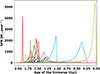 |
Fig. 1. Star formation histories of the QGs obtained by fitting a double power-law model using BAGPIPES. |
According to Weaver et al. (2023), the outlier fraction for galaxies with magnitudes between 22 and 25 is approximately 4%. Consequently, there is a 4% probability that MQGs may be misclassified at either lower or higher redshifts in the COSMOS 2020 catalogue, which might lead to their exclusion from our sample. Previous studies, such as Leja et al. (2019) and Carnall et al. (2018), have demonstrated that standard SFH models such as an exponentially declining SFH may systematically underestimate stellar masses. Using the LePHARE sSFR in the COSMOS2020 catalogue, we successfully recovered only 11 out of the 24 MQGs identified in our sample. Additionally, LePHARE predicts 5 additional MQGs that are classified as star-forming by our Bagpipes SED fitting. A visual inspection of the SEDs of these 5 sources revealed that they exhibit strong optical emission, indicating that they are not true MQGs. This suggests that LePHARE fails to properly constrain the SFR for these sources, which leads to a potential misclassification as compared to BAGPIPES.
2.6. Voronoi Monte Carlo map construction from the COSMOS2020 catalogue
We adopted the Voronoi Monte Carlo (VMC) mapping technique to measure the galaxy density in the entire COSMOS field within our redshift range. This approach has been thoroughly examined and validated in previous studies in the literature (eg. Shah et al. 2024; Hung et al. 2020; Lemaux et al. 2018; Cucciati et al. 2018; Forrest et al. 2020), and its robustness and reliability were demonstrated. The main advantage of the VMC mapping is its ability to cover a wide dynamical range in densities, that is, it allows us to detect very high and very low densities, without assuming any prior on the shape of the density field. Hence, it is a non-parametric and scale-independent method.
In the simple Voronoi tessellation method, a 2D plane is divided into a number of cells such that each cell is associated with an object. Each cell is defined as the collection of all the points closer to that object than to any other object. More crowded regions therefore have smaller cells than less crowded regions. The density associated with each cell is calculated using the area of each cell as explained below. To take the variation in redshift within our redshift range into account, we instead used the VMC technique described by Hung et al. (2020), which represents an improvement over the standard Voronoi technique. The resulting VMC map is shown in the left panel of Figure 2. The main steps are described below.
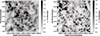 |
Fig. 2. Density map traced by the galaxies selected from the COSMOS2020 (left) and the LAE (right) catalogues, obtained by using the VMC technique (Section 2.3). The colour bar represents the normalised density calculated in Section 2.8. The red dots represent the MQGs. |
-
We constructed a series of overlapping redshift slices within our entire redshift range of 3.004 ≤ z ≤ 3.224. The width of each redshift slice (z-slice) was equal to the median uncertainty on the photometric redshift of our QG sample, that is, 0.04.
-
We assigned a photometric redshift probability weight to each galaxy in each slice. The percentage of the redshift probability distribution function (z-pdf) lying in the z-slice is the weight of a galaxy for a given slice. For this, we assumed that all galaxies have a Gaussian z-pdf.
-
We generated a random number for each galaxy. The random number lay between the minimum and the maximum weight of all the galaxies for a slice. When the weight of a galaxy was greater than the random number, it was accepted. Thus, we obtained a set of accepted galaxies for each z-slice.
-
For each z-slice, we then generated a simple Voronoi map. The average of all 12 z-slice Voronoi maps was the final Voronoi map we used.
2.7. Voronoi map construction from the ODIN-LAE catalogue
In order to create the LAE Voronoi map, we assumed that the redshifts of all our LAEs were fixed at z = 3.1 because the narrow-band technique used to find the LAEs is very secure, with a redshift range of 0.062 (Firestone et al. 2024). Of the ODIN LAEs with confident redshift measurements from DESI, ≈97% have the correct redshift classification for being in the N501 filter. The LAE map and the structures discovered therein were published by Ramakrishnan et al. (2023). The right panel of Figure 2 shows the LAE Voronoi map.
2.8. Density estimation from the Voronoi maps
Following the method described in the literature (e.g. Cucciati et al. 2018; Lemaux et al. 2018; Hung et al. 2020), we created a pixelated surface density map. This was done by populating the field with a uniform grid of points, where the grid spacing was set to ≈70 ckpc, which is much smaller than the Voronoi cells. Each pixel within a Voronoi cell was assigned a surface density. The surface density in a Voronoi cell (i, j), Σ(i, j), was calculated using the area of a Voronoi cell (Av) as follows:
 (3)
(3)
The normalised local density, (1 + δ), in a Voronoi cell (i, j) was then estimated as
 (4)
(4)
where Σ(i, j) is the density of a given Voronoi cell, and  is the median density of all the Voronoi cells in the redshift slice (Figure 2). As discussed in various studies, these local density estimates correlate well with other density metrics and accurately trace known overdensity structures. We repeated this process for the LAE Voronoi map to construct an LAE density map. As described by Ramakrishnan et al. (2023), the size of a pixel is ≈120 ckpc on a side for the LAE density map.
3. Results
3.1. Number density and physical properties of quiescent galaxies
We identified 24 QG candidates at z ≈ 3.1. One of these has previously been identified by Ito et al. (2023). The remaining 23 are promising new photometric candidates. Table A1 shows their best-fit physical properties.
The total survey volume without the star masks that is covered by the COSMOS2020 catalogue is 8.71 × 10⁵ cMpc3. We therefore calculated the number density of MQGs as  galaxies cMpc−3, which is consistent with the observed number densities reported in the literature (Straatman et al. 2014; Schreiber et al. 2018; Merlin et al. 2019; Carnall et al. 2023) and with estimates from simulations, such as IllustrisTNG300 (Valentino et al. 2020). We calculated the uncertainties following the method described by Gehrels (1986), which provides a procedure for estimating Poisson uncertainties in the regime of low number statistics.
The code BAGPIPES gives the SFH that best reproduces the observed photometry of a galaxy as an output. The code BAGPIPES estimates the time of formation (tform) and the time of quenching (tquench) for a galaxy. tform is defined as
Following the prescription of Carnall et al. (2018), we defined the quenching timescale as follows:
 (5)
(5)
Simulations have shown that the quenching timescale is one of the critical parameters that can be used to distinguish between various quenching mechanisms (Wright et al. 2019; Wetzel et al. 2013; Walters et al. 2022). For instance, stellar feedback from supernovae can quench a galaxy within 0.1 Gyr (Ceverino & Klypin 2009). In contrast, merger-driven quenching is expected to have a median delay time of approximately 1.5 Gyr, although this timescale can vary significantly (Rodríguez Montero et al. 2019). Figure 3 shows that 19 out of our 24 MQGs exhibit quenching timescales within a relatively narrow range of 300–500 Myr. The similarity in quenching timescales among the majority of our galaxies suggests that they may have been influenced by a common quenching mechanism. Simulations predict that mechanisms such as overconsumption (Walters et al. 2022), ram-pressure stripping (Steinhauser et al. 2016), stellar feedback (Ceverino & Klypin 2009), and AGN feedback (e.g, Hirschmann et al. 2017) operate on short timescales and are capable of rapidly quenchinggalaxies.
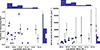 |
Fig. 3. Left: quenching timescale of the MQGs (as defined in Equation (3.1)) as a function of the stellar mass estimated using BAGPIPES. The median duration of the quenching is ≈350 Myr, and it is consistent for all MQGs. The log stellar mass (M⊙) is always ≥10.6. Right: SFR at the peak of the SFH of the MQG as a function of the stellar mass. The peak SFR increases linearly with mass, indicating a stronger starburst for more massive galaxies. |
One MQG exhibits a notably longer quenching timescale (≈0.9 Gyr) than the rest of the sample. The SED and SFH of this galaxy are presented in Figure C8. Unlike the rest, this galaxy may not have had to undergo a strong starburst in its SFH, and its SFR peak is only ≈150 M⊙ yr−1. This particular galaxy is an outlier and may have a different type of quenching mechanism. It lies in a slight higher than average local density, but not in a significant overdensity. It is possible that, in this case, environmental quenching processes with long timescales Mao et al. (2022) may have conditioned its evolution.
The quenching timescale in our analysis was derived from SED fitting of photometric data using a double power-law star formation history model, which may introduce some uncertainty in its estimation. Simulations based on the SIMBA framework have shown that this model can lead to offsets in the quenching timescale of up to 100 Myr, whereas the commonly used exponentially declining model can introduce biases as large as 400 Myr (Carnall et al. 2018). Future studies that combine both spectroscopic and photometric observations are crucial for placing tighter constraints on the quenching timescales.
3.2. Density maps at z = 3.1
The photo-z and LAE Voronoi maps are presented in Figure 2. Protoclusters are overdense structures in the early Universe that eventually evolved into present-day galaxy clusters. For the identification of these structures, we employed SEP (Barbary 2016), which is a Python implementation of the SExtractor software (Bertin & Arnouts 1996). The number of detected structures is highly dependent on the chosen detection threshold (DETECT_THRESH) and minimum area (DETECT_MINAREA). According to Chiang et al. (2013), a protocluster at redshift 3 is expected to have a minimum effective radius of 5 cMpc and a minimum halo mass of 1012 M⊙ for it to evolve into a cluster of Mhalo > 1014 M⊙ at z = 0.
Ramakrishnan et al. (2023) developed specific SExtractor criteria for the ODIN survey to identify protoclusters. They reported that a detection threshold (DETECT_THRESH) of 4.5σ and a minimum area (DETECT_MINAREA) of 3000 pixels (corresponding to approximately 40 cMpc2) results in a contamination rate of 20%. We adopted these criteria from Ramakrishnan et al. (2023) to identify protoclusters from the surface density maps to have a consistent detection procedure for the ODIN and COSMOS2020 map. For clarity, we use the term “protocluster” exclusively for overdense structures identified using this method because it was optimised for the detection of protoclusters. In Figure 4 we show the structures detected in the LAE and COSMOS2020 Voronoi maps.
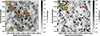 |
Fig. 4. Shaded yellow regions represent structures identified by running Source Extractor in the COSMOS2020 (left) and in the LAE (right) maps. The yellow dots represent MQGs. The colour bar scales the log(1 + δ) density for both maps as in Figure 2. Letters A, B, C, and D indicate some major overdensity groups that are discovered in either one or both maps. |
There are some important differences between the LAE and the COSMOS2020 map. To discuss them in detail, we name some of the protoclusters in capital letters. The large protoclusters at δ ≊ 2.3° (B and C in Figure 4) detected in the COSMOS2020 map are not detected in the LAE map. The large protocluster at α = 149.6° detected in the LAE map (D) is not detected in the COSMOS2020 map. The group of overdensities at α ≊ 150.6° (A) is detected in both maps. The reason for the difference in the appearance of the overdensities/protoclusters may be the redshift ranges. The photo-z galaxies are selected to be in the range 3.004 ≤ z ≤ 3.224, while the LAEs lie in a narrower range of Δz = 0.062, centred at z = 3.124 (Lee et al. 2024). Therefore, the new structures in the photo-z map could be just outside the very narrow range of the LAE map. The structures detected in the density maps are promising photometric protocluster candidates. Follow-up spectroscopy of the constituent galaxies of these protoclusters could confirm their exact redshift and 3D shape.
Only 6 of the 24 MQGs are located within protocluster candidates that were discovered in either the LAE or photoz maps, which represents just 25% of the MQG candidates. This suggests that processes that typically occur in dense environments may not always be necessary for galaxy quenching. This includes process that occur in the hot ICM, such as ram-pressure stripping (Boselli et al. 2022) and thermal evaporation (Cowie & Songaila 1977), and processes that have a higher probability of occurring in dense environments, such as galaxy harassment and strangulation.
We compared the location of MQGs with the location of the massive star-forming galaxies (MSFGs) in relation to the protocluster candidates. MSFGs are defined as star-forming galaxies with a stellar mass higher than 1010.6 M⊙. We performed this comparison at a fixed limit of stellar mass, so that mass segregation did not bias our comparison. Figure 5 displays the two distributions. To determine whether the MQGs and MSFGs follow the same distribution, we performed the Anderson-Darling test. We obtained a high p-value of ≈0.25 for both cases, which suggests that the two samples are statistically consistent with being drawn from the same distribution. This further indicates that MQGs follow the same distribution with respect to protoclusters as MSFGs. We interpret this as evidence that environmental processes, which are more common in protoclusters, are not the dominant quenching mechanism. We also performed this test without fixing the stellar mass limits and obtained a similar result. Figures 6 and 7 show the quenching timescale and the SFRpeak versus the environmental density in the photo-z map and the LAE map, respectively. We show that neither the quenching timescale nor the SFR at the peak of the SFH depends on the local density. This suggests that the mechanisms that cause star formation in MQGs do not significantly depend on the environment.
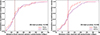 |
Fig. 5. Left: cumulative distribution of the distances of MQGs and MSFGs to the photo-z protocluster centers. Right: cumulative distribution of the distances of MQGs and MSFGs to the LAEs protocluster centres. The dotted lines show the median distribution for each type of galaxy. The p-value of the Anderson-Darling test that compared MQGs with the distribution of all galaxies is also displayed. MQGs and MSFGs were selected at the same stellar mass limit. |
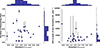 |
Fig. 6. Left: quenching timescale as a function of density from the COSMOS2020 VMC map. Right: SFR at peak of star formation as a function of density from the COSMOS2020 VMC map. |
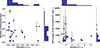 |
Fig. 7. Left: quenching timescale as a function of density from the LAE density map. Right: SFR at the peak of star formation as a function of density from the LAE density map. |
3.3. Quiescent fraction and the environment
The quiescent fraction is described as the proportion of MQGs to the count of MSFGs present within a specified density bin. We performed this calculation at a fixed stellar mass M > 1010.6 M⊙ to ensure a fair comparison between MSFGs and MQGs and did not introduce a mass bias in the results.
Figure 8 shows the quiescent fraction as a function of local density. By local density, we refer to the density within the pixel of the Voronoi map at which the MQG resides. The resolution of the photo-z density map and the LAE density map is 70 ckpc pixel−1 and 120 ckpc pixel−1, respectively. The uncertainty in the quiescent fraction was obtained using the method described by Gehrels (1986), who provided convenient tables and approximate formulas for calculating confidence limits based on Poisson and binomial statistics. This method is widely used in astronomy for estimating uncertainties with small-number statistics. We used Equations (10) and (12) from Gehrels (1986) to calculate these uncertainties, which provide the upper (λu) and lower limit (λl) to a measured quantity according to Poisson statistics as follows:
 (6)
(6)
 (7)
(7)
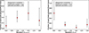 |
Fig. 8. Left: evolution of the quenched fraction with the local density, log(1+δ), in the COSMOS2020 density map. Right: evolution of the quenched fraction with the local density, log(1+δ), in the LAE density map. |
Here, n is the number of observed events (or counts). The confidence limits are calculated for the observed value. The value of S (a Poisson parameter) was listed by Gehrels (1986) for different confidence levels.
To quantify the observed correlation between the quenched fraction and the local density in the COSMOS2020 map and the LAE map, we employed the Spearman correlation coefficient. Taking into account the uncertainty in the quiescent fraction, we calculated a weighted Spearman coefficient. This involved bootstrapping the quenched fraction within the bounds of the uncertainty 3000 times. For each sample, we computed the Spearman correlation coefficient. Finally, we determined the mean and standard deviation of the computed coefficients, which provided a robust measure of the correlation while accounting for the associated uncertainties. We obtained a mean Spearman correlation coefficient of ≈0.43 and a standard deviation of ≈0.44. A Spearman coefficient of 0.43 signifies a weak or no correlation. To robustly confirm a correlation, the coefficient should exceed 0.7, while a value below 0.43 generally suggests the absence of a correlation. In our Monte Carlo simulations, we found that 43% of the runs resulted in a correlation coefficient below 0.4, and we therefore conclude that there is no dependence on the local density. To validate these statistical results, we performed simulations by generating samples with strong and weak correlations. Our findings indicate that a weak correlation can still be observed even with a small sample size of 24 when using weighted Spearman coefficients. Further details, including a more thorough examination of the correlation, can be found in the Appendix B. The independence of the quiescent fraction of the local density agrees with the analysis in Section 3.2, and it further suggests that quenching mechanisms in MQGs may not be driven by environmental processes alone.
3.4. Neighbor count
In the local Universe, environmental processes in galaxy groups and clusters play a significant role as quenching mechanism (Boselli & Gavazzi 2006). To investigate the environment of MQGs at different scales, we counted the number of nearest neighbours within 2D projected distances ranging from 0.1 to 6 cMpc for all photo-z selected galaxies and all MQGs. Table 2 presents the median values.
Number of neighbours of MQGs and all galaxies.
Figure F1 in the Appendix E shows the distribution of the number of neighbours for MQGs and for all galaxies in the COSMOS2020 catalogue.
Based on the median values, we conclude that MQGs and all galaxies have similar median values for their number of neighbours. This indicates that MQGs do not have a higher probability of residing in groups or overdense environments at various scales than star-forming galaxies. Secular quenching mechanisms, such as AGN feedback and stellar feedback, which do not necessarily depend on the environment, may play a dominant role in the quenching of galaxies at this epoch at z = 3.1.
3.5. Filaments
Filaments traced by LAEs are recognised as substantial reservoirs of cold gas that can sustain star formation in galaxies. Consequently, it is anticipated that star-forming galaxies are located on or close to these filaments. Conversely, a negative correlation is expected between MQGs and filaments because galaxies situated near filaments benefit from a continuous supply of cold gas that is conducive to star formation. Ramakrishnan et al. (2023) identified these filaments within the COSMOS field using LAEs and the code called discrete persistent structure extractor (DisPerSE) code (Sousbie 2011).
It is crucial to note that the redshift range of the LAEs that was used to trace these filaments is very narrow, specifically, Δz = 0.062. We lack the precise spectroscopic redshift for MQGs and photo-z selected galaxies from the COSMOS2020 catalogue. The redshift range for our MQGs and photo-z selected galaxies is wider and spans 3.1 ± 0.12. As a result, we can only compute the 2D projected distances of our photo-z sample galaxies relative to the filaments. These distances are measured in arcseconds, where at z = 3.1, 1″ corresponds to 31.27 ckpc. We compared the distributions of MQGs and the MSFGs at z = 3.1 using the Anderson-Darling test. Figure 9 displays the filaments detected in the COSMOS field with LAEs. It illustrates the spatial distribution of the MQGs relative to these filaments.
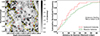 |
Fig. 9. Left: filaments (yellow lines) discovered using DisPerSE by Ramakrishnan et al. (2023), overplotted on the LAE density map. The red points represent the MQGs. Right: cumulative distribution of the distances to the nearest filaments for MQGs and MSFGs. |
We applied the Anderson-Darling test to assess whether the distribution of MQGs and MSFGs with respect to the filaments differs significantly. The test yielded a p-value of 0.18, which exceeds common significance thresholds (0.05, 0.01). Consequently, we find no statistically significant difference between the two samples. The median distances of MQGs and photo-z galaxies from the filaments are 9 and 11 cMpc, respectively. This similarity suggests that the probability of a galaxy to be quenched does not depend on its proximity to a filament. We also find that some MQGs lay in proximity to gas-rich LAE filaments. Specifically, 9 out of 24 MQGs are located within 5 cMpc of a filament. Filaments are typically rich in cold gas and represent significant reservoirs for star formation (Martizzi et al. 2019). For these MQGs, their proximity to these gas-rich filaments therefore implies that processes involving gas heating, such as virial shock heating or AGN feedback, may be actively suppressing star formation by hindering the accretion of cold gas.
4. Discussion
We have searched for QGs at z ≈ 3.1, studied their physical properties, and investigated their relation with the environment. We discovered 24 MQGs that are characterised by log sSFR < −10.01 in a 2 deg2 area of the COSMOS field. The number density of the MQGs is  galaxies/cMpc3, and it is consistent with observations and simulations in the literature (Valentino et al. 2020).
We characterised the environment in the COSMOS field and considered two independent tracers: LAEs; and the general galaxy population of the COSMOS2020 catalogue, using the Voronoi tessellation. While some overdense structures are common in both these maps, there are large overdense structures that are discovered in only one of the two maps. The reason for this difference might be the differnt redshift precision in the two samples. We selected galaxies from the COSMOS2020 catalogue on the basis of photometric redshifts. The range of this photo-z was ≈3–3.2. This migh lead to an overdensity detection that is not co-spatial with LAE-traced structures, whose redshift range is very narrow (Δz = 0.06, z ≈ 3.1).
Our study identified two protoclusters that we called B and C and that are present in the photo-z map, but absent in the LAE map. Forrest et al. (2023) have discovered protoclusters at positions similar to B and C at a slightly higher redshift (z ≈ 3.32), named S3 and S1 in their analysis. We propose that these two protoclusters detected in our photo-z map might also be the front-end extension of the S1 and S3 protoclusters. Our LAE observations may not have fully captured certain overdensities due to the inherently narrow redshift coverage (Δz ≈ 0.062) of the narrow-band selection method. Beyond observational constraints, however, there may be important astrophysical factors underlying the discrepancies observed between structures traced by LAEs and those identified using broader photometric selection methods. Specifically, the population of LAEs is known to not fully overlap with luminous Lyman-break galaxies (LBGs), MQGs, or dusty star-forming galaxies, as each population tends to occupy distinct evolutionary stages, host halo masses, and environmental contexts.
Previous studies (e.g. Overzier 2016; Shi et al. 2020; Shimakawa et al. 2017) have highlighted that LAEs typically trace younger lower-mass galaxies associated with gas-rich environments or filamentary structures. In contrast, photometrically selected galaxy populations, such as MQGs and dusty galaxies, often trace more massive haloes and potentially more evolved dynamically mature environments (e.g. Shi et al. 2019; Calvi et al. 2023). Consequently, different galaxy populations may reveal overdensities at different evolutionary stages or spatial scales within the cosmic web. These differences emphasise the complexity of interpreting galaxy overdensities identified by varying selection methods and caution against the assumption that these methods sample identical physical environments or evolutionary phases.
Further multi-wavelength observational campaigns, in particular, spectroscopic follow-up across various galaxy populations, are necessary to fully elucidate the astrophysical reasons for these differences and to clarify the connection between different galaxy populations and their underlying large-scalestructures.
The LAEs are detected using the narrow-band excess created by the Lyman-α emission line. The absorption of the resonant Lyman-alpha line in a dusty and highly overdense region might make it harder to detect LAEs. The Lyman-alpha IGM transmission is a complex function that is significantly influenced by the geometry and density of the IGM (Gurung-López et al. 2019, 2020). This small-scale effect may obscure certain parts of structures, such as extremely overdense and dusty centres of some protoclusters, but it is unlikely to miss entire protoclusters, as seen in our maps. The photo-z density map complements the LAE density map because the precision of photo-z-selected galaxies is similar to that of the MQGs.
Our analysis showed that only 20% of our MQGs are located in protoclusters. The spatial distribution of QGs relative to protocluster centres is similar to that of the general galaxy population. Therefore, MQGs do not show a higher tendency to be found in protoclusters than other types of galaxies. As noted in Section 3.4, MQGs have a comparable number of neighbours within the entire range from 0.5 to 6 Mpc as the general galaxy population, that is, they lie in a very similar environment. This suggests that environmental mechanisms prevalent in protoclusters or galaxy groups, such as ram-pressure stripping, galaxy–galaxy interactions, strangulation, harassment, tidal stripping, and thermal evaporation, are not alone the cause for the quenching MQGs.
Some studies using IllustrisTNG simulation furthermore showed that environmental processes such as mergers do not cause the quenching of galaxies at high redshift. Kurinchi-Vendhan et al. (2024) found that merger events do not significantly distinguish between quiescent and star-forming galaxies in the IllustrisTNG300 simulation and are unlikely to drive galaxy quenching at z > 3. Their study concluded that quenched galaxies have experienced longer and more intense AGN activity, which released larger amounts of thermal energy than star-forming galaxies prior to quenching.
Our findings are broadly consistent with the emerging picture that high-redshift galaxy quenching operates on rapid timescales and is primarily driven by internal processes. Recent work by Tacchella et al. (2022) reinforced the notion that stellar feedback, alongside contributions from AGN, can dramatically curtail star formation during the early phases of galaxy assembly. These feedback mechanisms appear to be especially effective in massive haloes, such as those of MQGs.
We find that MQGs are not correlated with local peaks in the environmental density, as illustrated in Figure 8. The quenched fraction remains nearly constant across a wide range of environmental densities, suggesting that quenching mechanisms may operate independently of local density variations. Additionally, 7 of 24 MQGs are located in regions with an exceptionally high density that are characterised by δ > 2. Since high-density regions also serve as reservoirs of cold gas, mechanisms to heat the gas are necessary to prevent a further accretion of cold gas that would rejuvenate the MQGs. In this context, AGN feedback is a plausible quenching mechanism.
The feedback of AGN is a secular quenching mechanism that can quench galaxies in a wide range of environments. AGN outflows cause the expulsion of gas from the gravitational bounds of their host galaxies, which reduces the subsequent star formation activity (DeBuhr et al. 2012; Combes 2017). Additionally, AGNs can heat the cool gas in the interstellar medium, which further prevents the formation of new stars (Croton et al. 2006; Man & Belli 2018; Zinger et al. 2020). Recently, several observational studies using JWST and ALMA have found signs of gas outflows driven by AGN in MQGs at z > 3 in morphological and spectroscopic observations (Kubo et al. 2022; Ito et al. 2022; Park et al. 2024). Park et al. (2024), Glazebrook et al. (2024), D’Eugenio et al. (2023), Ito et al. (2022), Kubo et al. (2022) have found multi-phase outflows and neutral gas outflows in MQGs along with evidence of AGN. Ito et al. (2022) reported ubiquitous AGN activity in MQGs up to z = 5. Nanayakkara et al. (2025) presented spectroscopic evidence that linked high-redshift MQGs to powerful AGN activity, consistent with the scenario that short-lived starbursts (and the subsequent quenching) may be triggered or accelerated by the presence of an AGN. In this context, quenching as a result of AGN feedback is consistent with our observation that MQGs are not correlated with protoclusters and have a similar number of neighbours as other types of galaxies.
In their study using the Magneticum simulation, Kimmig et al. (2025) also found that galaxies are quenched before cosmic noon (z = 3.42) primarily because gas is removed by AGN feedback. Kimmig et al. (2025) predicted that the quenching process is also influenced by the environment, however. They showed that for a galaxy to be quenched, it must reside in a significant underdensity that prevents the replenishment of cold gas. In contrast to their study, we did not observe any preference for MQGs to reside in underdense regions. Instead, MQGs exhibit a random distribution with respect to protoclusters, suggesting that the effect of the environment may not be significant for quenching at a redshift of approximately 3.1.
Filaments traced by LAEs are reservoirs of neutral gas that can rejuvenate galaxies even when a starburst has consumed the entire gas. We did not observe an anti-correlation between the position of MQGs and filaments. In fact, 25% of our MQGs occur within 5 cMpc of gas-rich filaments. This might be an indication of the action of physical processes that heat the gas near the galaxies, preventing the accretion of cold gas. This might further indicate that AGN heat the gas around the galaxies. Kalita et al. (2021) highlighted the importance of internal processes such as AGN feedback and morphological stabilisation, where bulge growth can help to suppress gas inflows and ultimately halt star formation. This aligns well with our inference that several of our MQGs reside in environments with potentially abundant gas (e.g. near filaments and in protoclusters), but remain quenched, presumably due to heating or outflows that circumvent fresh gas accretion.
By performing SED fitting, we obtained the SFH of our MQGs. It is typically characterised by a starburst phase, followed by a quenching period, with a timescale shorter than 500 Myr (Figure 3). The uniformity in the duration of quenching of these galaxies suggests that they were quenched by the same mechanism and physical processes, which are probably not strictly related to the environment. This quenching mechanism would include a massive starburst that consumes gas rapidly, along with a mechanism that prevents the inflow of cold gas to maintain star formation. A rapid quenching phase has been observed in other studies in the literature, such as Whitaker et al. (2012), Wild et al. (2016), Schreiber et al. (2018), Carnall et al. (2018), D’Eugenio et al. (2020), Carnall et al. (2023). Quenching timescales obtained from the simulations (e.g. Wright et al. 2019; Wetzel et al. 2013; Walters et al. 2022) can help us to distinguish between the quenching mechanisms. In general, we can distinguish quenching into fast-quenching mechanisms (≈0.1 Gyr) and slow-quenching (≈1 Gyr) mechanisms. Furthermore, any trend in the quenching timescale with environment density can indicate the dependence of the quenching mechanism on the local environment. Environmental processes that are typically much slower are therefore unlikely to quench these galaxies (Mao et al. 2022).
Figure 6 showed that the time it takes to quench a galaxy is not strongly correlated with the density of the local environment. A similar result was found in Figure 7, which showed the quenching timescale with respect to LAE densities. No correlation between quenching timescale and the environment indicates that the environment alone may not be the significant driver of quenching. Similarly, the right panel of Figures 6 and 7 show that the SFRpeak and the environment density are not correlated. We conclude that the SFH and hence the processes that quenched these MQGs do not depend strongly on the environment.
In order to spectroscopically confirm the redshift and obtain a more precise constraint on the SFH and stellar mass, it is essential to acquire spectra. JWST NIRSpec follow-up observations can be used to spectroscopically confirm MQGs at z ≈ 3.1. Follow-up observations with the JWST NIRSpec will be instrumental in identifying AGN-driven outflows as well as neutral gas outflows, which may play a role in quenching star formation. Furthermore, a morphological analysis using NIRCam would provide valuable insight into the impact of mergers on dense environments.
5. Conclusions
We presented a detailed analysis of 24 QGs identified at z ≈ 3.1 within the 2-deg2 COSMOS field using deep photometric data from the COSMOS2020 catalogue. These galaxies are characterised by high stellar masses exceeding 1010.6 M⊙. Our spectral energy distribution fitting revealed that these MQGs exhibit remarkably consistent star-formation histories that are characterised by intense early starburst episodes that were rapidly followed by quenching within short timescales of ≤400 Myr. The similarity in the quenching timescales in the entire sample strongly suggests a universal and highly efficient quenching mechanism that operated at cosmic noon.
By examining galaxy environments using Voronoi-based density maps constructed independently from photometrically selected COSMOS2020 galaxies and ODIN-selected LAEs, we found no significant correlation between galaxy quenching parameters (quenching duration, quenched fraction, or timing) and local environmental density. Furthermore, MQGs do not exhibit a preferential distribution with respect to protoclusters or cosmic filaments compared to similarly MSFGs. This indicates that purely environmental processes alone (e.g. ram-pressure stripping, galaxy mergers, or harassment) may not dominate galaxy quenching at this epoch. The presence of MQGs within environments that are expected to be rich in cold gas, such as protoclusters and filaments, further implies that simple gas exhaustion might not be the sole contributor to quenching, and gas-heating mechanisms induced by AGN or stellar feedback might also play significant roles.
Our findings support the hypothesis that internal mechanisms such as AGN feedback, stellar feedback-driven gas heating, virial shock heating, or morphological quenching might play a more dominant role in galaxy quenching at these redshifts. Future spectroscopic confirmation of the precise redshifts of these galaxies is crucial to securely associate them with identified protoclusters and filaments. Additionally, detailed studies of gas dynamics and gas ionisation states within and around MQGs using integral-field spectroscopy (e.g. MUSE) and interferometric observations (e.g, ALMA) in diverse environments are essential. These observations can confirm the availability, temperature, and ionisation state of the gas reservoirs and clarify the contributions of gas heating and exhaustion. Spectroscopic follow-up to confirm the presence and strength of AGN activity in MQGs will further test our proposed hypothesis regarding dominant internal quenching mechanisms that operated during this critical epoch of galaxy evolution.
Acknowledgments
AS and LG acknowledge the FONDECYT regular project number 1230591 for financial support. EG and KSL acknowledge support from NSF grants AST-2206222, AST-2206705, and AST-2408359. Based on observations at Cerro Tololo Inter-American Observatory, NSF’s NOIRLab (NOIRLab Prop. ID 2020B0201; PI: K.-S. Lee), which is managed by the Association of Universities for Research in Astronomy (AURA) under a cooperative agreement with the National Science Foundation. LG also gratefully acknowledges financial support from ANID – MILENIO – NCN2024_112 and the ANID BASAL project FB210003. This work made use of the computer server RAGNAR at Universidad Andres Bello.
References
- Aihara, H., AlSayyad, Y., Ando, M., et al. 2019, PASJ, 71, 114 [Google Scholar]
- Arnouts, S., Cristiani, S., Moscardini, L., et al. 1999, MNRAS, 310, 540 [Google Scholar]
- Barbary, K. 2016, J. Open Source Software, 1, 58 [NASA ADS] [CrossRef] [Google Scholar]
- Bertin, E., & Arnouts, S. 1996, A&AS, 117, 393 [NASA ADS] [CrossRef] [EDP Sciences] [Google Scholar]
- Boselli, A., & Gavazzi, G. 2006, PASP, 118, 517 [Google Scholar]
- Boselli, A., Fossati, M., & Sun, M. 2022, A&ARv, 30, 3 [NASA ADS] [CrossRef] [Google Scholar]
- Bressan, A., Marigo, P., Girardi, L., et al. 2012, MNRAS, 427, 127 [NASA ADS] [CrossRef] [Google Scholar]
- Bruzual, G., & Charlot, S. 2003, MNRAS, 344, 1000 [NASA ADS] [CrossRef] [Google Scholar]
- Calvi, R., Castignani, G., & Dannerbauer, H. 2023, A&A, 678, A15 [NASA ADS] [CrossRef] [EDP Sciences] [Google Scholar]
- Calzetti, D., Armus, L., Bohlin, R. C., et al. 2000, ApJ, 533, 682 [NASA ADS] [CrossRef] [Google Scholar]
- Carnall, A. C., McLure, R. J., Dunlop, J. S., & Davé, R. 2018, MNRAS, 480, 4379 [Google Scholar]
- Carnall, A., McLeod, D., McLure, R., et al. 2023, MNRAS, 520, 3974 [NASA ADS] [CrossRef] [Google Scholar]
- Casey, C. M. 2016, ApJ, 824, 36 [CrossRef] [Google Scholar]
- Ceverino, D., & Klypin, A. 2009, ApJ, 695, 292 [Google Scholar]
- Chevallard, J., & Charlot, S. 2016, MNRAS, 462, 1415 [NASA ADS] [CrossRef] [Google Scholar]
- Chiang, Y.-K., Overzier, R., & Gebhardt, K. 2013, ApJ, 779, 127 [Google Scholar]
- Cicone, C., Maiolino, R., Sturm, E., et al. 2014, A&A, 562, A21 [NASA ADS] [CrossRef] [EDP Sciences] [Google Scholar]
- Combes, F. 2017, Front. Astron. Space Sci., 4, 10 [NASA ADS] [CrossRef] [Google Scholar]
- Cowie, L. L., & Songaila, A. 1977, Nature, 266, 501 [Google Scholar]
- Croton, D. J., Springel, V., White, S. D., et al. 2006, MNRAS, 365, 11 [NASA ADS] [CrossRef] [Google Scholar]
- Cucciati, O., Lemaux, B., Zamorani, G., et al. 2018, A&A, 619, A49 [NASA ADS] [CrossRef] [EDP Sciences] [Google Scholar]
- Davé, R., Thompson, R., & Hopkins, P. F. 2016, MNRAS, 462, 3265 [Google Scholar]
- DeBuhr, J., Quataert, E., & Ma, C.-P. 2012, MNRAS, 420, 2221 [NASA ADS] [CrossRef] [Google Scholar]
- D’Eugenio, C., Daddi, E., Gobat, R., et al. 2020, ApJ, 892, L2 [Google Scholar]
- D’Eugenio, F., Perez-Gonzalez, P., Maiolino, R., et al. 2023, ArXiv e-prints [arXiv:2308.06317] [Google Scholar]
- Dressler, A. 1980, ApJ, 236, 351 [Google Scholar]
- Dunlop, J. S., Bowler, R. A., Franx, M., et al. 2023, A Decade of ESO Wide-field Imaging Surveys (surveys2023), 10 [Google Scholar]
- Fabian, A. C. 2012, ARA&A, 50, 455 [Google Scholar]
- Falcón-Barroso, J., Sánchez-Blázquez, P., Vazdekis, A., et al. 2011, A&A, 532, A95 [Google Scholar]
- Firestone, N. M., Gawiser, E., Ramakrishnan, V., et al. 2024, ApJ, 974, 217 [Google Scholar]
- Forrest, B., Annunziatella, M., Wilson, G., et al. 2020, ApJ, 890, L1 [NASA ADS] [CrossRef] [Google Scholar]
- Forrest, B., Lemaux, B. C., Shah, E., et al. 2023, MNRAS, 526, L56 [NASA ADS] [CrossRef] [Google Scholar]
- Gawiser, E., Francke, H., Lai, K., et al. 2007, ApJ, 671, 278 [NASA ADS] [CrossRef] [Google Scholar]
- Gehrels, N. 1986, ApJ, 303, 336 [Google Scholar]
- Girelli, G., Bolzonella, M., & Cimatti, A. 2019, A&A, 632, A80 [NASA ADS] [CrossRef] [EDP Sciences] [Google Scholar]
- Glazebrook, K., Schreiber, C., Labbé, I., et al. 2017, Nature, 544, 71 [Google Scholar]
- Glazebrook, K., Nanayakkara, T., Marchesini, D., Kacprzak, G., & Jacobs, C. 2022, Proc. Int. Astron. Union, 18, 3 [Google Scholar]
- Glazebrook, K., Nanayakkara, T., Marchesini, D., Kacprzak, G., & Jacobs, C. 2024, in Early Disk-Galaxy Formation from JWST to the Milky Way, eds. F. Tabatabaei, B. Barbuy, & Y. S. Ting, 377, 3 [Google Scholar]
- Gunn, J. E., & Gott, J. R., III 1972, ApJ, 176, 1 [Google Scholar]
- Gurung-López, S., Orsi, Á. A., Bonoli, S., Baugh, C. M., & Lacey, C. G. 2019, MNRAS, 486, 1882 [Google Scholar]
- Gurung-López, S., Orsi, Á. A., Bonoli, S., et al. 2020, MNRAS, 491, 3266 [Google Scholar]
- Hartley, A. I., Nelson, E. J., Suess, K. A., et al. 2023, MNRAS, 522, 3138 [Google Scholar]
- Hirschmann, M., Charlot, S., Feltre, A., et al. 2017, MNRAS, 472, 2468 [NASA ADS] [CrossRef] [Google Scholar]
- Hu, E. M., & McMahon, R. G. 1996, Nature, 382, 231 [Google Scholar]
- Hung, D., Lemaux, B., Gal, R., et al. 2020, MNRAS, 491, 5524 [NASA ADS] [CrossRef] [Google Scholar]
- Ito, K., Tanaka, M., Miyaji, T., et al. 2022, ApJ, 929, 53 [NASA ADS] [CrossRef] [Google Scholar]
- Ito, K., Tanaka, M., Valentino, F., et al. 2023, ApJ, 945, L9 [NASA ADS] [CrossRef] [Google Scholar]
- Jin, S., Daddi, E., Liu, D., et al. 2018, ApJ, 864, 56 [Google Scholar]
- Jin, S., Sillassen, N. B., Magdis, G. E., et al. 2024, A&A, 683, L4 [NASA ADS] [CrossRef] [EDP Sciences] [Google Scholar]
- Kalita, B., Daddi, E., D’Eugenio, C., et al. 2021, ApJ, 917, L17 [NASA ADS] [CrossRef] [Google Scholar]
- Kimmig, L. C., Remus, R.-S., Seidel, B., et al. 2025, ApJ, 979, 15 [Google Scholar]
- Kovač, K., Somerville, R. S., Rhoads, J. E., Malhotra, S., & Wang, J. 2007, ApJ, 668, 15 [Google Scholar]
- Kubo, M., Umehata, H., Matsuda, Y., et al. 2022, ApJ, 935, 89 [NASA ADS] [CrossRef] [Google Scholar]
- Kurinchi-Vendhan, S., Farcy, M., Hirschmann, M., & Valentino, F. 2024, MNRAS, 534, 3974 [NASA ADS] [CrossRef] [Google Scholar]
- Larson, R. B. 1990, PASP, 102, 709 [Google Scholar]
- Le Fèvre, O., Cassata, P., Cucciati, O., et al. 2013, A&A, 559, A14 [Google Scholar]
- Lee, K.-S., Gawiser, E., Park, C., et al. 2024, ApJ, 962, 36 [Google Scholar]
- Leja, J., Carnall, A. C., Johnson, B. D., Conroy, C., & Speagle, J. S. 2019, ApJ, 876, 3 [Google Scholar]
- Lemaux, B., Cucciati, O., Tasca, L., et al. 2014, A&A, 572, A41 [NASA ADS] [CrossRef] [EDP Sciences] [Google Scholar]
- Lemaux, B. C., Le Fèvre, O., Cucciati, O., et al. 2018, A&A, 615, A77 [NASA ADS] [CrossRef] [EDP Sciences] [Google Scholar]
- Liu, D., Lang, P., Magnelli, B., et al. 2019, ApJS, 244, 40 [Google Scholar]
- Man, A., & Belli, S. 2018, Nat. Astron., 2, 695 [NASA ADS] [CrossRef] [Google Scholar]
- Mao, Z., Kodama, T., Pérez-Martínez, J. M., et al. 2022, A&A, 666, A141 [NASA ADS] [CrossRef] [EDP Sciences] [Google Scholar]
- Marigo, P., Girardi, L., Bressan, A., et al. 2017, ApJ, 835, 77 [Google Scholar]
- Martizzi, D., Vogelsberger, M., Artale, M. C., et al. 2019, MNRAS, 486, 3766 [Google Scholar]
- McCracken, H., Milvang-Jensen, B., Dunlop, J., et al. 2012, A&A, 544, A156 [NASA ADS] [CrossRef] [EDP Sciences] [Google Scholar]
- Merlin, E., Fortuni, F., Torelli, M., et al. 2019, MNRAS, 490, 3309 [CrossRef] [Google Scholar]
- Moore, B., Katz, N., Lake, G., Dressler, A., & Oemler, A. 1996, Nature, 379, 613 [Google Scholar]
- Nanayakkara, T., Glazebrook, K., Jacobs, C., et al. 2024, Sci. Rep., 14, 3724 [NASA ADS] [CrossRef] [Google Scholar]
- Nanayakkara, T., Glazebrook, K., Schreiber, C., et al. 2025, ApJ, 981, 78 [Google Scholar]
- Ouchi, M., Shimasaku, K., Furusawa, H., et al. 2003, ApJ, 582, 60 [Google Scholar]
- Ouchi, M., Ono, Y., & Shibuya, T. 2020, ARA&A, 58, 617 [Google Scholar]
- Overzier, R. A. 2016, A&ARv, 24, 14 [Google Scholar]
- Pacifici, C., Oh, S., Oh, K., Lee, J., & Sukyoung, K. Y. 2016, ApJ, 824, 45 [NASA ADS] [CrossRef] [Google Scholar]
- Park, C., & Hwang, H. S. 2009, ApJ, 699, 1595 [NASA ADS] [CrossRef] [Google Scholar]
- Park, M., Belli, S., Conroy, C., et al. 2024, ApJ, 976, 72 [Google Scholar]
- Peng, Y., Lilly, S. J., Kovač, K., et al. 2010, ApJ, 721, 193 [NASA ADS] [CrossRef] [Google Scholar]
- Ramakrishnan, V., Moon, B., Im, S. H., et al. 2023, ApJ, 951, 119 [NASA ADS] [CrossRef] [Google Scholar]
- Rodríguez Montero, F., Davé, R., Wild, V., Anglés-Alcázar, D., & Narayanan, D. 2019, MNRAS, 490, 2139 [CrossRef] [Google Scholar]
- Salim, S., & Narayanan, D. 2020, ARA&A, 58, 529 [NASA ADS] [CrossRef] [Google Scholar]
- Sanchez-Blazquez, P., Peletier, R., Jimenez-Vicente, J., et al. 2006, MNRAS, 371, 703 [CrossRef] [Google Scholar]
- Sawicki, M., Arnouts, S., Huang, J., et al. 2019, MNRAS, 489, 5202 [NASA ADS] [Google Scholar]
- Schreiber, C., Glazebrook, K., Nanayakkara, T., et al. 2018, A&A, 618, A85 [NASA ADS] [CrossRef] [EDP Sciences] [Google Scholar]
- Scoville, N., Aussel, H., Brusa, M., et al. 2007, ApJS, 172, 1 [Google Scholar]
- Shah, E. A., Lemaux, B., Forrest, B., et al. 2024, MNRAS, 529, 873 [NASA ADS] [CrossRef] [Google Scholar]
- Shi, K., Huang, Y., Lee, K.-S., et al. 2019, ApJ, 879, 9 [NASA ADS] [CrossRef] [Google Scholar]
- Shi, K., Toshikawa, J., Cai, Z., Lee, K.-S., & Fang, T. 2020, ApJ, 899, 79 [Google Scholar]
- Shimakawa, R., Kodama, T., Hayashi, M., et al. 2017, MNRAS, 468, L21 [NASA ADS] [CrossRef] [Google Scholar]
- Sousbie, T. 2011, MNRAS, 414, 350 [NASA ADS] [CrossRef] [Google Scholar]
- Spitler, L. R., Straatman, C. M., Labbé, I., et al. 2014, ApJ, 787, L36 [NASA ADS] [CrossRef] [Google Scholar]
- Steinhauser, D., Schindler, S., & Springel, V. 2016, A&A, 591, A51 [NASA ADS] [CrossRef] [EDP Sciences] [Google Scholar]
- Straatman, C. M., Labbé, I., Spitler, L. R., et al. 2014, ApJ, 783, L14 [NASA ADS] [CrossRef] [Google Scholar]
- Tacchella, S., Finkelstein, S. L., Bagley, M., et al. 2022, ApJ, 927, 170 [NASA ADS] [CrossRef] [Google Scholar]
- Tanaka, M., Onodera, M., Shimakawa, R., et al. 2024, ApJ, 970, 59 [Google Scholar]
- Valentino, F., Tanaka, M., Davidzon, I., et al. 2020, ApJ, 889, 93 [Google Scholar]
- Walters, D., Woo, J., & Ellison, S. L. 2022, MNRAS, 511, 6126 [NASA ADS] [CrossRef] [Google Scholar]
- Weaver, J., Davidzon, I., Toft, S., et al. 2023, A&A, 677, A184 [NASA ADS] [CrossRef] [EDP Sciences] [Google Scholar]
- Weaver, J. R., Kauffmann, O., Shuntov, M., et al. 2021, Am. Astron. Soc. Meet. Abstr., 53, 215.06 [NASA ADS] [Google Scholar]
- Wetzel, A. R., Tinker, J. L., Conroy, C., & Van Den Bosch, F. C. 2013, MNRAS, 432, 336 [NASA ADS] [CrossRef] [Google Scholar]
- Whitaker, K. E., Kriek, M., van Dokkum, P. G., et al. 2012, ApJ, 745, 179 [CrossRef] [Google Scholar]
- Wild, V., Almaini, O., Dunlop, J., et al. 2016, MNRAS, 463, 832 [NASA ADS] [CrossRef] [Google Scholar]
- Williams, R. J., Quadri, R. F., Franx, M., van Dokkum, P., & Labbé, I. 2009, ApJ, 691, 1879 [NASA ADS] [CrossRef] [Google Scholar]
- Wright, R. J., Lagos, C. D. P., Davies, L. J., et al. 2019, MNRAS, 487, 3740 [NASA ADS] [CrossRef] [Google Scholar]
- Zinger, E., Pillepich, A., Nelson, D., et al. 2020, MNRAS, 499, 768 [CrossRef] [Google Scholar]
Appendix A: Galaxy properties
Galaxy Properties
Galaxy Properties-2
Appendix B: Simulations to check the validity of correlation
In Figure 8, we plot the quenched fraction versus the local density on the COSMOS2020 and LAE maps. We perform a test to investigate whether our current data are sufficient to detect the presence (or absence) of a correlation between the quenched fraction and the local density.
To quantify the discriminating power of our dataset, we select galaxies and designate them as ’MQGs’. We select 6 sets of galaxies, each containing 25, 50, 100, 200, 250, and 300 galaxies, respectively. These galaxies are not selected entirely randomly. We first select sets with a "strong correlation" with the local density. They are selected such that:
-
70 % of the set lies in highly overdense regions (δ>3)
-
20 % of the set lies in overdense region (2 < δ < 3)
-
5 % of the set lies in average density region (1 < δ < 2)
-
5 % of the set lies in underdense region (δ < 1)
We then calculate the ’quenched fraction’ using the selected galaxies. We calculate the Spearman correlation coefficient using the Monte Carlo technique defined in Section 3.3. We display the results of the exercise in Table B1.
From this simulation, we conclude that if a strong correlation existed, we would be able to find it using our analysis, even with a relatively small sample of 24 galaxies. However, for a smaller sample of galaxies (up to 100), the Spearman correlation coefficient is overestimated and finally converges for 150 or more sources. The mean correlation coefficient calculated for our sample in Section 3.3 is 0.55 and therefore we can confidently rule out the presence of a strong correlation between the quenched fraction and the environmental density.
We repeat this analysis for a weakly correlated sample generated such that:
-
15 % of the set lies in highly overdense regions (δ > 3)
-
20 % of the set lies in overdense region (2 < δ < 3)
-
45 % of the set lies in average density region (1 < δ < 2)
-
20 % of the set lies in underdense region (δ < 1)
In this weakly correlated sample, we can also see a correlation at a median ≈0.6. The Spearman correlation coefficient increases with an increase in the number of selected sources. From these simulations, we conclude that if a correlation existed, we would be able to find it using our analysis, even with a relatively small sample of 24 galaxies, as in the main part of this paper. Further notable is that even for a small number of sources, no more than 22% of the Monte Carlo runs show no correlation (SC< 0.4). In this case too, for a small number of sources, the correlation coefficient can be overestimated, with nearly 50% of the Monte Carlo predictions incorrectly showing a strong correlation. This is different from our calculations in Section 3.3 where nearly 45% of Monte Carlo, where SC< 0.4. We conclude from this that there exists no correlation between quenched fraction and the environment density.
The statistics obtained for the strongly correlated simulated sample.
The statistics obtained for weakly correlated samples.
Appendix C: SEDs and SFH of MQGs
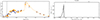 |
Fig. C1. SED and SFH for COSMOS ID 412439 |
 |
Fig. C2. SED and SFH for COSMOS ID 13648 |
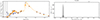 |
Fig. C3. SED and SFH for COSMOS ID 20998 |
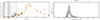 |
Fig. C4. SED and SFH for COSMOS ID 50248 |
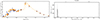 |
Fig. C5. SED and SFH for COSMOS ID 110859 |
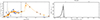 |
Fig. C6. SED and SFH for COSMOS ID 278297 |
 |
Fig. C7. SED and SFH for COSMOS ID 282964 |
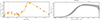 |
Fig. C8. SED and SFH for COSMOS ID 310229 |
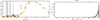 |
Fig. C9. SED and SFH for COSMOS ID 341682 |
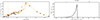 |
Fig. C10. SED and SFH for COSMOS ID 343373 |
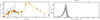 |
Fig. C11. SED and SFH for COSMOS ID 383298 |
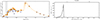 |
Fig. C12. SED and SFH for COSMOS ID 405872 |
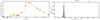 |
Fig. C13. SED and SFH for COSMOS ID 489177 |
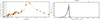 |
Fig. C14. SED and SFH for COSMOS ID 642338 |
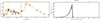 |
Fig. C15. SED and SFH for COSMOS ID 658452 |
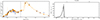 |
Fig. C16. SED and SFH for COSMOS ID 706985 |
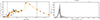 |
Fig. C17. SED and SFH for COSMOS ID 779869 |
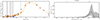 |
Fig. C18. SED and SFH for COSMOS ID 803389 |
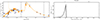 |
Fig. C19. SED and SFH for COSMOS ID 881980 |
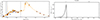 |
Fig. C20. SED and SFH for COSMOS ID 911001 |
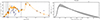 |
Fig. C21. SED and SFH for COSMOS ID 961549 |
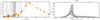 |
Fig. C22. SED and SFH for COSMOS ID 962569 |
[width = 0.5]962569fit.tif
 |
Fig. C23. SED and SFH for COSMOS ID 338392 |
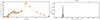 |
Fig. C24. SED and SFH for COSMOS ID 681407 |
Appendix D: Corner Plots for SED fitting
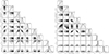 |
Fig. D1. Corner plot for COSMOS ID 13648 and 20998 |
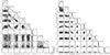 |
Fig. D2. Corner plot for COSMOS ID 50248 and 110859 |
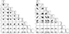 |
Fig. D3. Corner plot for COSMOS ID 278297 and 282964 |
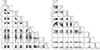 |
Fig. D4. Corner plot for COSMOS ID 310229 and 338392 |
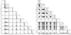 |
Fig. D5. Corner plot for COSMOS ID 341682 and 343373 |
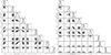 |
Fig. D6. Corner plot for COSMOS ID 383298 and 405872 |
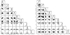 |
Fig. D7. Corner plot for COSMOS ID 412439 and 489177 |
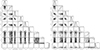 |
Fig. D8. Corner plot for COSMOS ID 642338 and 658452 |
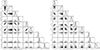 |
Fig. D9. Corner plot for COSMOS ID 681407 and 706985 |
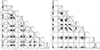 |
Fig. D10. Corner plot for COSMOS ID 779869 and 803389 |
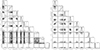 |
Fig. D11. Corner plot for COSMOS ID 881980 and 911001 |
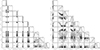 |
Fig. D12. Corner plot for COSMOS ID 961549 and 962569 |
Appendix E: Nearest neighbours
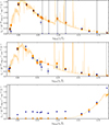 |
Fig. E1. Examples of galaxies rejected from the MQG sample after visual inspection. |
Appendix F: Visual inspection of galaxies
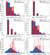 |
Fig. F1. Number of neighbours within radii of 0.1-6 Mpc for all galaxies and MQGs. The vertical line represents the mean of the distributions. |
All Tables
Priors of the free parameters of the BAGPIPES model that we used to fit the photometric data.
All Figures
|
Fig. 1. Star formation histories of the QGs obtained by fitting a double power-law model using BAGPIPES. |
| In the text | |
|
Fig. 2. Density map traced by the galaxies selected from the COSMOS2020 (left) and the LAE (right) catalogues, obtained by using the VMC technique (Section 2.3). The colour bar represents the normalised density calculated in Section 2.8. The red dots represent the MQGs. |
| In the text | |
|
Fig. 3. Left: quenching timescale of the MQGs (as defined in Equation (3.1)) as a function of the stellar mass estimated using BAGPIPES. The median duration of the quenching is ≈350 Myr, and it is consistent for all MQGs. The log stellar mass (M⊙) is always ≥10.6. Right: SFR at the peak of the SFH of the MQG as a function of the stellar mass. The peak SFR increases linearly with mass, indicating a stronger starburst for more massive galaxies. |
| In the text | |
|
Fig. 4. Shaded yellow regions represent structures identified by running Source Extractor in the COSMOS2020 (left) and in the LAE (right) maps. The yellow dots represent MQGs. The colour bar scales the log(1 + δ) density for both maps as in Figure 2. Letters A, B, C, and D indicate some major overdensity groups that are discovered in either one or both maps. |
| In the text | |
|
Fig. 5. Left: cumulative distribution of the distances of MQGs and MSFGs to the photo-z protocluster centers. Right: cumulative distribution of the distances of MQGs and MSFGs to the LAEs protocluster centres. The dotted lines show the median distribution for each type of galaxy. The p-value of the Anderson-Darling test that compared MQGs with the distribution of all galaxies is also displayed. MQGs and MSFGs were selected at the same stellar mass limit. |
| In the text | |
|
Fig. 6. Left: quenching timescale as a function of density from the COSMOS2020 VMC map. Right: SFR at peak of star formation as a function of density from the COSMOS2020 VMC map. |
| In the text | |
|
Fig. 7. Left: quenching timescale as a function of density from the LAE density map. Right: SFR at the peak of star formation as a function of density from the LAE density map. |
| In the text | |
|
Fig. 8. Left: evolution of the quenched fraction with the local density, log(1+δ), in the COSMOS2020 density map. Right: evolution of the quenched fraction with the local density, log(1+δ), in the LAE density map. |
| In the text | |
|
Fig. 9. Left: filaments (yellow lines) discovered using DisPerSE by Ramakrishnan et al. (2023), overplotted on the LAE density map. The red points represent the MQGs. Right: cumulative distribution of the distances to the nearest filaments for MQGs and MSFGs. |
| In the text | |
|
Fig. C1. SED and SFH for COSMOS ID 412439 |
| In the text | |
|
Fig. C2. SED and SFH for COSMOS ID 13648 |
| In the text | |
|
Fig. C3. SED and SFH for COSMOS ID 20998 |
| In the text | |
|
Fig. C4. SED and SFH for COSMOS ID 50248 |
| In the text | |
|
Fig. C5. SED and SFH for COSMOS ID 110859 |
| In the text | |
|
Fig. C6. SED and SFH for COSMOS ID 278297 |
| In the text | |
|
Fig. C7. SED and SFH for COSMOS ID 282964 |
| In the text | |
|
Fig. C8. SED and SFH for COSMOS ID 310229 |
| In the text | |
|
Fig. C9. SED and SFH for COSMOS ID 341682 |
| In the text | |
|
Fig. C10. SED and SFH for COSMOS ID 343373 |
| In the text | |
|
Fig. C11. SED and SFH for COSMOS ID 383298 |
| In the text | |
|
Fig. C12. SED and SFH for COSMOS ID 405872 |
| In the text | |
|
Fig. C13. SED and SFH for COSMOS ID 489177 |
| In the text | |
|
Fig. C14. SED and SFH for COSMOS ID 642338 |
| In the text | |
|
Fig. C15. SED and SFH for COSMOS ID 658452 |
| In the text | |
|
Fig. C16. SED and SFH for COSMOS ID 706985 |
| In the text | |
|
Fig. C17. SED and SFH for COSMOS ID 779869 |
| In the text | |
|
Fig. C18. SED and SFH for COSMOS ID 803389 |
| In the text | |
|
Fig. C19. SED and SFH for COSMOS ID 881980 |
| In the text | |
|
Fig. C20. SED and SFH for COSMOS ID 911001 |
| In the text | |
|
Fig. C21. SED and SFH for COSMOS ID 961549 |
| In the text | |
|
Fig. C22. SED and SFH for COSMOS ID 962569 |
| In the text | |
|
Fig. C23. SED and SFH for COSMOS ID 338392 |
| In the text | |
|
Fig. C24. SED and SFH for COSMOS ID 681407 |
| In the text | |
|
Fig. D1. Corner plot for COSMOS ID 13648 and 20998 |
| In the text | |
|
Fig. D2. Corner plot for COSMOS ID 50248 and 110859 |
| In the text | |
|
Fig. D3. Corner plot for COSMOS ID 278297 and 282964 |
| In the text | |
|
Fig. D4. Corner plot for COSMOS ID 310229 and 338392 |
| In the text | |
|
Fig. D5. Corner plot for COSMOS ID 341682 and 343373 |
| In the text | |
|
Fig. D6. Corner plot for COSMOS ID 383298 and 405872 |
| In the text | |
|
Fig. D7. Corner plot for COSMOS ID 412439 and 489177 |
| In the text | |
|
Fig. D8. Corner plot for COSMOS ID 642338 and 658452 |
| In the text | |
|
Fig. D9. Corner plot for COSMOS ID 681407 and 706985 |
| In the text | |
|
Fig. D10. Corner plot for COSMOS ID 779869 and 803389 |
| In the text | |
|
Fig. D11. Corner plot for COSMOS ID 881980 and 911001 |
| In the text | |
|
Fig. D12. Corner plot for COSMOS ID 961549 and 962569 |
| In the text | |
|
Fig. E1. Examples of galaxies rejected from the MQG sample after visual inspection. |
| In the text | |
|
Fig. F1. Number of neighbours within radii of 0.1-6 Mpc for all galaxies and MQGs. The vertical line represents the mean of the distributions. |
| In the text | |
Current usage metrics show cumulative count of Article Views (full-text article views including HTML views, PDF and ePub downloads, according to the available data) and Abstracts Views on Vision4Press platform.
Data correspond to usage on the plateform after 2015. The current usage metrics is available 48-96 hours after online publication and is updated daily on week days.
Initial download of the metrics may take a while.