| Issue |
A&A
Volume 700, August 2025
|
|
|---|---|---|
| Article Number | A181 | |
| Number of page(s) | 9 | |
| Section | Planets, planetary systems, and small bodies | |
| DOI | https://doi.org/10.1051/0004-6361/202452760 | |
| Published online | 15 August 2025 | |
KMT-2024-BLG-0404L: A triple microlensing system consisting of a star, a brown dwarf, and a planet
1
Department of Physics, Chungbuk National University,
Cheongju
28644,
Republic of Korea
2
Astronomical Observatory, University of Warsaw,
Al. Ujazdowskie 4,
00-478
Warszawa,
Poland
3
Korea Astronomy and Space Science Institute,
Daejon
34055,
Republic of Korea
4
University of Canterbury, Department of Physics and Astronomy,
Private Bag 4800,
Christchurch
8020,
New Zealand
5
Max Planck Institute for Astronomy,
Königstuhl 17,
69117
Heidelberg,
Germany
6
Department of Astronomy, The Ohio State University,
140 W. 18th Ave.,
Columbus,
OH
43210,
USA
7
Center for Astrophysics | Harvard & Smithsonian
60 Garden St.,
Cambridge,
MA
02138,
USA
8
Department of Particle Physics and Astrophysics, Weizmann Institute of Science,
Rehovot
76100,
Israel
9
Department of Astronomy, Tsinghua University,
Beijing
100084,
China
10
Center for Cosmology and AstroParticle Physics, Ohio State University,
191 West Woodruff Ave.,
Columbus,
OH
43210,
USA
11
Department of Physics, University of Warwick,
Gibbet Hill Road,
Coventry,
CV4 7AL,
UK
12
Villanova University, Department of Astrophysics and Planetary Sciences,
800 Lancaster Ave.,
Villanova,
PA
19085,
USA
★ Corresponding author: This email address is being protected from spambots. You need JavaScript enabled to view it.
Received:
26
October
2024
Accepted:
7
July
2025
Abstract
Aims. We have investigated the lensing event KMT-2024-BLG-0404. The light curve of the event exhibited a complex structure with multiple distinct features, including two prominent caustic spikes, two cusp bumps, and a brief discontinuous feature between the caustic spikes. While a binary-lens model captured the general anomaly pattern, it could not account for a discontinuous anomaly feature between the two caustic spikes.
Methods. To explore the origin of the unexplained feature, we conducted more advanced modeling beyond the standard binary-lens framework. This investigation demonstrated that the previously unexplained anomaly was resolved by introducing an additional lens component with planetary mass.
Results. The estimated masses of the lens components are Mp = 17.3−8.8+25.5 ME for the planet, and Mh,A = 0.090−0.046+0.133 M⊙ and Mh,B = 0.026−0.013+0.038 M⊙ for the binary host stars. Based on these mass estimates, the lens system is identified as a planetary system where a Uranus-mass planet orbits a binary consisting of a late M dwarf and a brown dwarf. The distance to the planetary system is estimated to be DL = 7.21−0.97+0.93 kpc, with an 82% probability that it resides in the Galactic bulge. This discovery represents the ninth planetary system found through microlensing with a planet orbiting a binary host. Notably, it is the first case in which the host consists of both a star and a brown dwarf.
Key words: planets and satellites: detection
© The Authors 2025
 Open Access article, published by EDP Sciences, under the terms of the Creative Commons Attribution License (https://creativecommons.org/licenses/by/4.0), which permits unrestricted use, distribution, and reproduction in any medium, provided the original work is properly cited.
This article is published in open access under the Subscribe to Open model. This email address is being protected from spambots. You need JavaScript enabled to view it. to support open access publication.
1 Introduction
Microlensing is a technique that can detect planets orbiting around binary stars. Microlensing discoveries of these planets are possible because both the planetary companion and the binary companion to the primary lens produce distinct signals. Consequently, the presence of a planet and the binary nature of the host can be identified for a fraction of events in which the source passes through the perturbation region created by both lens companions. Han (2008) was the first to propose the potential of using the microlensing technique to detect planets in binary star systems. Since that time, eight microlensing planetary systems within binaries have been reported.
The first microlensing planet in a binary system was discovered by Gould et al. (2014) through the analysis of the OGLE-2013-BLG-0341 lensing event. The binary nature of the lens was recognized from an anomaly near the peak of the event’s light curve and a small bump that appeared well before the peak. The planetary signal was detected as a dip in the light curve on the rising side of the event. The planet, with a mass approximately twice that of Earth, is located at a projected separation comparable to the distance between the Earth and the Sun. Its host star orbits a slightly more massive companion with a projected separation of about 10 to 15 AU.
The second microlensing planet in a binary system was discovered through the analysis of the lensing event OGLE-2008-BLG-092 by Poleski et al. (2014). In this microlensing event, distinct signals from both the binary stellar and planetary companions to the primary were identified, each explainable by the light curve of a single-mass object. The planet, which has a mass approximately four times that of Uranus, orbits a binary system composed of a K dwarf and an M dwarf.
The third microlensing planet in a binary was identified by Bennett et al. (2016) through their analysis of the lensing event OGLE-2007-BLG-349. The peak part of the lensing light curve in this event clearly indicated a signal from a planet, while an additional signal hinted at the presence of another lensing mass. Their analysis provided two plausible model interpretations: one suggesting two planets orbiting a single star, and the other proposing a circumbinary planet. The ambiguity between these models was resolved by detecting excess flux from the binary-lens star system using Hubble Space Telescope imaging. The planet identified is a gas giant orbiting a pair of M dwarfs.
Han et al. (2017) reported the discovery of the fourth planet in a binary system through an analysis of the lensing event OGLE-2016-BLG-0613. The light curve displayed the typical features of a caustic-crossing binary-lens event, with two caustic spikes and a U-shaped trough between them. However, an additional short-term, discontinuous feature appeared within the trough. A detailed analysis uncovered three possible models, all suggesting that this extra feature was produced by a planetary companion to the binary lens. The primary star’s mass was most likely around 0.7 M⊙, and the planet was classified as a super-Jupiter, although the mass of the binary companion varies depending on the models.
The fifth planetary system, OGLE-2006-BLG-284L, was reported by Bennett et al. (2020) following a detailed analysis of the microlensing event OGLE-2006-BLG-284. In this event, the planetary signal appeared as a brief but distinct deviation from the typical two-spike light curve seen in a caustic-crossing binary-lens event. A thorough analysis confirmed that this short-term signal was caused by a planetary companion. The lens system consists of a giant planet orbiting a pair of M dwarf stars. This discovery further highlighted microlensing’s ability to detect planetary companions in binary star systems.
The sixth microlensing planet in a binary system was discovered through the analysis of the lensing light curve of OGLE-2018-BLG-1700. In this event, the signals from both the stellar and planetary companions overlapped in the central region, leading to a complex anomaly in the peak region of the light curve. Han et al. (2020) characterized the triple nature of the lens by separating the anomaly pattern into two distinct components, each corresponding to a binary-lens event. One binary-lens pair exhibited a mass ratio of approximately 0.01 between the lens objects, suggesting that the companion is a planet, while the other had a mass ratio of about 0.3. Through Bayesian analysis, they estimated the mass of the planetary companion to be around four times that of Jupiter, with the stellar binary components having masses of approximately 0.4 M⊙ and 0.12 M⊙.
The seventh triple-lens system consisting of a planet and a binary was identified by Zang et al. (2021) through the analysis of central anomalies in the lensing event KMT-2020-BLG-0414. They found that the planet has an extremely low mass, similar to that of Earth. From a subsequent follow-up observation using Keck adaptive optics, Zhang et al. (2024) found that the planet is hosted by a binary composed of a brown dwarf and a white dwarf, as is evidenced by the non-detection of the lens flux.
The last microlensing planet in a binary stellar system was discovered by Han et al. (2024) through their analysis of the lensing event OGLE-2023-BLG-0836. Similar to the event OGLE-2018-BLG-1700, the anomaly displayed central deviations of a complex anomaly pattern that could not be explained by a binary-lens model. This anomaly could be explained by a triple-lens model in which one member of the lens is a planet. The planet has a mass 4.4 times that of Jupiter, and the stellar binary consists of two stars with masses of approximately 0.7 M⊙ and 0.6 M⊙.
Interpreting the lensing behavior of a planet in a binary system requires modeling a triple-lens system. The lensing behavior of a triple-lens system was first introduced by Grieger et al. (1989), who explored the impact of shear caused by a third body and demonstrated the resulting complexity in the caustic structure. Rhie (2002) later showed that the lens equation for a triple-lens system is a two-dimensional vector equation, which can be embedded into a tenth-order analytic polynomial equation in one complex variable. Han et al. (2001) demonstrated that the anomalies induced by multiple planets could be approximated by superimposing the anomalies from individual planets. The first triple-lens system, OGLE-2006-BLG-109L, consisting of two planets orbiting a low-mass star (Gaudi et al. 2008), was interpreted through this approach. The complexities of modeling a triple-lens system were thoroughly examined by Danĕk & Heyrovský (2015) and Danĕk & Heyrovský (2019). These complexities were illustrated by the analysis of the lensing event OGLE-2013-BLG-0723, in which the lens responsible for the light curve was initially interpreted as a triple system, including a Venus, a brown dwarf, and a star (Udalski et al. 2015b), but later reinterpreted as a rotating binary system (Han et al. 2016).
We conducted a project involving a detailed analysis of anomalous microlensing events identified by the Korea Microlensing Telescope Network (KMTNet) survey (Kim et al. 2016). The aim of the project is to investigate events with anomalies in their light curves that cannot be explained by the conventional binary-lens single-source (2L1S) or single-lens binary-source (1L2S) models. Through this analysis, we identified cases requiring more advanced modeling beyond the standard 2L1S or 1L2S frameworks. In most cases, these complex anomalies were resolved by introducing additional lens or source components. Previous events with light curves interpreted using four-body (lens+source) models are listed in Table 1 of Han et al. (2023). In this paper, we report an additional planet in a binary system, discovered through a systematic investigation of KMTNet data from the 2024 season.
2 Observation and data
The planetary system was discovered through a detailed analysis of the microlensing event KMT-2024-BLG-0404. The KMTNet group detected this event on April 3, 2024, corresponding to the abbreviated Heliocentric Julian date HJD′ = HJD – 2460000 = 403. The event’s baseline I-band magnitude was measured at Ibase = 18.63. The source is located at equatorial coordinates (RA, DEC)J2000 = (18:04:35.30, –27:57:12.60), corresponding to Galactic coordinates (l, b) = (2°.9528, –3°. 1045). The source lies in the overlapping region of KMTNet prime fields BLG03 and BLG43. However, data from the BLG03 field were unavailable, as the source fell into the gap between the four camera chips.
The event was also independently detected and announced on April 11, 2024, by the Optical Gravitational Lensing Experiment group (OGLE; Udalski et al. 2015a), which designated it as OGLE-2024-BLG-0378.
In our analysis, we utilized combined data from both the KMTNet and OGLE surveys. KMTNet data were collected using three identical 1.6-meter telescopes located on three different continents in the southern hemisphere, allowing for continuous monitoring of microlensing events. These telescopes are situated at Cerro Tololo Inter-American Observatory in Chile (KMTC), Siding Spring Observatory in Australia (KMTA), and the South African Astronomical Observatory (KMTS). Each telescope is equipped with a camera covering a 4-square-degree field of view. Data from the OGLE survey were acquired using the 1.3-meter Warsaw telescope at Las Campanas Observatory in Chile, which features a 1.4-square-degree field of view. Both KMTNet and OGLE primarily observed in the I band, with approximately 10% of images taken in the V band for source color measurement.
The reduction of images and photometry for the lensing event was carried out using automated pipelines specific to each survey. For the KMTNet survey, image reduction was performed using the pipeline developed by Albrow et al. (2000), while the OGLE survey used the pipeline developed by Udalski (2003). To ensure optimal data quality, we conducted additional photometric analysis on the KMTNet data using a code developed by Yang et al. (2024). For both datasets, we rescaled the error bars to match the data scatter and normalized the χ2 per degree of freedom to unity, following the procedure described by Yee et al. (2012).
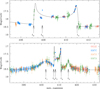 |
Fig. 1 Light curve of the lensing event KMT-2024-BLG-0404. The lower panel presents the overall view, while the upper panel provides a close-up of the caustic-crossing features. The curve overlaid on the data points represents the best-fit 2L1S model, which was derived by excluding data from the interval 407.5 < HJD′ < 408.0. In the lower panel, arrows labeled t1, t2, t3, t4, and t5 mark the positions of specific anomaly features. |
3 Light curve analysis
Figure 1 presents the lensing light curve for the event KMT-2024-BLG-0404, combining data from the OGLE and KMTNet surveys. The light curve displays a complex pattern with multiple anomaly features. First, the sharp rise and fall at times t2 and t4 correspond to a pair of spikes caused by the source crossing a caustic. Second, the smooth rise and fall at times t1 and t5 appear as bumps, likely due to the source approaching a caustic cusp. Additionally, a notable feature near t3 likely involves a caustic, as is indicated by the abrupt change in magnitude in the data between HJD′ = 407.7 and 407.9. In a two-mass lens system, the caustic forms a closed curve, and in the light curve of a caustic-crossing 2L1S event, the region between the two spikes typically forms a smooth “U”-shaped profile. The discontinuity at t3 in the trough strongly suggests the presence of a third mass in the lens system.
3.1 Binary-lens model
To analyze the caustic-related features, we began with a 2L1S model analysis of the light curve, aiming to determine the lens-ing solution – a set of parameters that best explains the observed light curve. A 2L1S event is characterized by seven fundamental parameters. Three of these parameters describe the source’s approach to the lens: t0 represents the time of closest approach of the source to the lens, u0 is the projected separation between the source and the lens at that moment, scaled to the angular Einstein radius (θΕ), and tE is the event timescale, defined as the time it takes for the source to cross θΕ. Two additional parameters describe the binary lens: s, the projected separation between the lens components (Ml and M2), scaled by θΕ, and q, the mass ratio between the two components. The parameter α indicates the angle of the source’s trajectory relative to the binary axis. Finally, ρ, defined as the ratio of the source radius (θ*) to the angular Einstein radius, accounts for finite-source effects, which lead to magnification attenuation during caustic crossings or approaches.
The modeling process employed a combination of grid and downhill methods. Due to the complexity of the χ2 surface for the 2L1S lensing parameters, relying solely on a downhill approach can be challenging. To tackle this, we conducted modeling with (s, q) as grid parameters, employing multiple starting values for α, while optimizing the remaining parameters using a downhill approach. Setting (s, q) as grid parameters is also crucial for exploring degenerate solutions, in which similar light curves may result from solutions with vastly different lensing parameters. In the downhill approach, we employed a Markov chain Monte Carlo (MCMC) algorithm. For the local solutions identified through this procedure, we subsequently refined the lensing parameters by allowing them to vary.
The 2L1S modeling yields a solution that captures the overall pattern of the anomaly, with the exception of the feature around t3. Figure 1 displays the model curve corresponding to the 2L1S solution derived from this analysis. The binary parameters for this solution are approximately (s, q) ~ (1.6,3.5), indicating that the lens is a binary consisting of two masses with a projected separation slightly exceeding the Einstein radius. The event timescale is tE ~ 11 days. The timescales corresponding to the individual lens components are given by tE,l = [1/(1 + q)]l/2tE ~ 5.3 days and tE,2 = [q/(l + q)]l/1tE ~ 9.9 days. These relatively short timescales suggest that the masses of the binary-lens components are likely to be small. The complete set of lensing parameters for the model is provided in Table 1.
Figure 2 illustrates the configuration of the 2L1S lens system, depicting the source trajectory with respect to the lens components and the resulting caustic. The lens generates a single resonant caustic with six cusps elongated along the binary axis. The source passes diagonally through the caustic, creating a spike at t2 upon entry and another spike at t4 upon exit. The bumps at t1 and t5 occur as the source approaches the upper right and lower left cusps of the caustic, respectively. In the figure, we mark the positions of the source at the moments of these major anomaly features. However, between t2 and t4, there is no caustic feature that could account for the anomaly seen in the lensing light curve around t3, indicating that the 2L1S model is insufficient to fully explain all the observed anomaly features.
Lensing parameters of the 2L1S model.
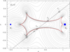 |
Fig. 2 Lens system configuration corresponding to the best-fit 2L1S model. The cuspy closed red figure represents the caustic, while the two blue dots labeled M1 and M2 denote the positions of the binary-lens components. The arrowed line illustrates the trajectory of the source. The four empty circles, scaled to the source size, mark the source positions along its trajectory at the times corresponding to the anomaly features at t1, t2, t4, and t5. The gray curves surrounding the caustic represent the equi-magnification contours. |
3.2 Triple-lens model
The fact that the discontinuous feature near t3 cannot be explained by a 2L1S model suggests an additional cause of the observed anomaly. We explore two possible explanations. The first is the existence of an additional companion to the source, resulting in a system composed of two lens masses and two source stars (a 2L2S event). Such configurations have been observed in events such as MOA-2010-BLG-117 (Bennett et al. 2018), KMT-2018-BLG-1743 (Han et al. 2021a), OGLE-2016-BLG-1003 (Jung et al. 2017), KMT-2019-BLG-0797 (Han et al. 2021b), KMT-2021-BLG-1898 (Han et al. 2022), OGLE-2018-BLG-0584, and KMT-2018-BLG-2119 (Han et al. 2023). The second possibility involves an additional companion to the lens, leading to a system with three lens masses and a single source star (a 3L1S event), as is illustrated by the events discussed in Sect. 1. Given that the anomaly around t3 constitutes a minor perturbation, in the 3L1S scenario the lens companion is likely to be a very low-mass object, while in the 2L2S scenario the source companion would probably be a faint star.
Of the two four-body (lens + source) models tested, we reject the 2L2S interpretation. The primary reason is that the 2L1S model leaves both positive and negative residuals in the data from the night of HJD′ = 407, whereas an additional source can only account for positive deviations. As a result, while the data point at HJD′ = 407.92 with a positive deviation could be explained by a 2L2S model, the remaining nine points with negative deviations (one from OGLE and eight from KMTC) cannot. This is illustrated in Figure 4, which presents the best-fit 2L2S model and its residuals. Given that the time interval between the two caustic spikes at t2 and t4 is relatively short (approximately 4 days) and that all features except for the one around t4 are described well by a static model, the anomaly near t3 is not attributed to lens or source orbital motion.
The 3L1S modeling was conducted in two phases. In the first phase, we performed a grid search focused on the parameters related to the third lens mass (M3), while keeping the parameters for the other two lens masses fixed to the values determined from the 2L1S modeling. The three parameters for M3 are (s3, q3), which represent the projected separation and mass ratio between M3 and M1, respectively, and ψ, which indicates the orientation of M3 relative to the M1–M2 axis. This method is viable because the 2L1S model describes the overall light curve pattern well, allowing the anomaly near t3 to be treated as a perturbation. In the second phase, we refined the lensing parameters for the local solutions identified from the χ2 surface of the grid search.
Figure 3 shows the Δχ2 map on the log s3–log q3 plane, revealing a distinct local minimum. The complete set of lensing parameters for the refined 3L1S model is listed in Table 2. The parameters of the second lens component remain nearly identical to the ones of the 2L1S model, indicating that the third mass causes only a small perturbation to the lensing system. The derived parameters for the third mass are approximately (s3, q3) ~ (0.63,1.9 × 10–3), suggesting that the third body is a planetary-mass object located within the Einstein ring of the host binary. The planet is positioned between the two binary components, with an orientation angle of –17.48 degrees measured at the location of M1 relative to the M1–M2 axis.
Figure 4 shows the model curve for the 3L1S solution in the region around the two caustic spikes. For comparison, the 2L1S model curve is also displayed (dotted line). It shows that the 3L1S model describes well the anomaly feature around t3, which could not be explained by the 2L1S model. The lens system configuration for the 3L1S solution is illustrated in Figure 5. The configuration appears similar to that of the 2L1S solution, as is expected from the similarity in lensing parameters, except for the ones related to M3. The third lens component generates a small caustic that distorts the upper fold of the main caustic induced by the binary. The planet-induced caustic resembles a pair of peripheral caustics created by a planet with a separation less than the Einstein radius (Han 2006). In this case, the region between the pair of peripheral caustics exhibits negative deviations. The observed negative deviations around t3 occurred as the source passed through this area.
To illustrate the correlations among the lensing parameters, we present scatter plots of the MCMC chain points for the 2L1S and 3L1S models in Figures A.1 and A.2, respectively.
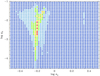 |
Fig. 3 Map of Δχ2 on the log s3–log q3 parameter surface derived from the triple-lens modeling. The color coding indicates points with Δχ2 ≤ 1nσ (red), ≤ 2nσ (yellow), ≤ 3nσ (green), ≤ 4nσ (cyan), and ≤ 5nσ (blue), where n = 4. |
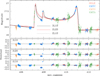 |
Fig. 4 Comparison of the models (2L1S, 2L2S, and 3L1S) in the region around caustic spikes. The lower panels show the residuals from the models. |
Lensing parameters of the 3L1S model.
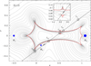 |
Fig. 5 Lens system configuration for the 3L1S model. The notations are the same as in Fig. 2. The inset presents a close-up of the area surrounding the planet-induced caustics. In comparison to the configuration shown in Fig. 2, the position of the third lens component (M3) and the source position at time t3 are additionally indicated. |
4 Source star and angular Einstein radius
We identified the source star of the event by measuring its dered-dened color and magnitude. Identifying the source star is crucial not only for fully characterizing the event, including the source, but also for measuring the angular Einstein radius. The Einstein radius is estimated as
 (1)
(1)
where the angular source radius (θ*) is inferred from the color and magnitude, and the normalized source radius is obtained from the modeling. For KMT-2024-BLG-0404, the value of ρ was measured from the analysis of the data during caustic crossings at t2, t3, and t4.
In order to estimate the reddening-corrected source color and magnitude, (V – I, I)0, from its instrumental values, (V – I, I), we used the Yoo et al. (2004) method, which utilizes the centroid of the red giant clump (RGC) in the color-magnitude diagram (CMD) as a reference for calibration (Rattenbury 2007). According to the method, we first measured (V – I, I) by regressing the V and I-band photometry data processed using the pyDIA photometry code (Albrow 2017) with respect to the model light curve. We then positioned the source in the instrumental CMD, constructed using the same pyDIA code, for stars located near the source in the KMTC image. The dereddened values of the source color and magnitude were then estimated as
 (2)
(2)
where (V – I, I)RGC,0 denote the dereddened color and magnitude of the RGC centroid and Δ(V – I, I) denote the offsets in color and magnitude of the source from the RGC centroid.
Figure 6 shows the positions of both the source and the RGC centroid in the CMD of stars located near the source. The measured instrumental color and magnitude of the source are
 (3)
(3)
and for the RGC centroid,
 (4)
(4)
With the offsets Δ(V – I, I) = (–0.260, 4.161) and the dereddened values for the RGC centroid, (V – I, I)RGC,0 = (1.060,14.606) (Bensby et al. 2013; Nataf et al. 2013), the estimated dereddened color and magnitude of the source are
 (5)
(5)
These values suggest that the source is a late G-type main-sequence star located in the Galactic bulge.
Using the measured color and magnitude, the angular radius of the source was determined based on the Kervella et al. (2004) relation. Because this relation is between (V – K, V) and θ*, we converted the measured V – I color into V – K using the color-color relation from Bessell & Brett (1988). The angular source radius estimated from this procedure is
 (6)
(6)
Combining the measured normalized source radius with the angular source radius yields an angular Einstein radius of
 (7)
(7)
Using this, along with the measured event timescale, the relative lens-source proper motion was calculated as
 (8)
(8)
The Einstein radii corresponding to the individual lens components M1 and M2 are θE,1 = [1/(1 + q)]1/2θΕ ~ 0.06 mas and θE,2 = [q/(1 + q)]1/2θE ~ 0.11 mas, respectively. These values are notably smaller than the typical Einstein radius of around 0.5 mas, which is commonly observed in lensing events caused by an M dwarf with a mass of approximately 0.3 M⊙ located midway between the observer and the source. Moreover, they align with the short event timescales, tE,1 ~ 5.3 days and tE,2 ~ 9.9 days.
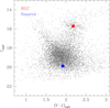 |
Fig. 6 Positions of the source and the centroid of the RGC in the instrumental CMD of stars lying near the source. |
5 Physical lens parameters
We estimated the physical parameters of the lens mass (M) and the distance to the planetary system (DL) based on the constraints provided by the lensing observables, specifically the event timescale and the angular Einstein radius. These observables are related to M and DL through the relations
 (9)
(9)
Here κ = 4G/(c2AU), πrel = AU(1/DL – 1/DS) represents the relative lens-source parallax, and DS is the distance to the source. In addition to these observables, the physical lens parameters can be further constrained by the microlens parallax (πΕ), which can be measured from the deviations in the light curve caused by Earth’s orbital motion around the Sun (Gould 1992). However, for KMT-2024-BLG-0404, this additional lensing observable of the microlens parallax could not be measured due to the event’s short timescale.
We determined the physical lens parameters through a Bayesian analysis. In the first step of this analysis, we generated a large sample of artificial lensing events (6 × 10⁶) using a Monte Carlo simulation. In this simulation, the lens mass was inferred from a model mass function, and the distances to the lens and source, along with their relative proper motion, were derived from a Galaxy model. For the mass function, we adopted the model from Jung et al. (2021), and for the Galaxy model, we used the Jung et al. (2021) model. For each artificial event, we computed the lensing observables, tΕ,i·and θE,i, corresponding to the physical lens parameters using the relations in Eq. (9). The Bayesian posteriors for the lens mass and distance were then constructed by imposing a weight, wi, on each artificial event. The weight was computed with
 (10)
(10)
where (tE, θE) and represent the measured values of the observables and [(σ(tΕ), σ(θΕ))] denote their uncertainties.
The Bayesian posteriors for the lens mass and the distances to both the lens and the source are shown in Figure 7. We also present the posterior for the source distance to show the relative positions of the lens and source. It should be noted that the mass posterior corresponds to the most massive lens component, M2. The estimated masses of the lens components are:
 (11)
(11)
Here the median was selected as the central value, with the 16th and 84th percentiles of the posterior distribution used to define the lower and upper uncertainty bounds, respectively. Based on the estimated masses of the lens components, the system is identified as a planetary system in which a Neptune-mass planet orbits within a binary consisting of a late M dwarf and a brown dwarf. The estimated distance to the lens is
 (12)
(12)
The planetary system is most likely located in the bulge, with an 82% probability. The projected separation between the binary components (M1 and M2) is  AU, while the planet is located at a separation of
  AU from M1. To ensure dynamical stability in the system, the planet should orbit only one of the host stars, and the separation between the binary components must be considerably greater than the distance from the planet to its host. This implies that the similarity between a⊥,2 and a⊥,3 is likely due to the projection effect.
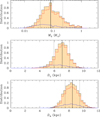 |
Fig. 7 Bayesian posteriors for the mass of the heaviest lens component (M2), distances to the lens and source (DL and DS). In each distribution, the solid vertical line represents the median value, while the 1σ uncertainty range is indicated by two dotted lines. The curves shown in blue and red represent the contributions from the disk and bulge lens populations, respectively, while the black line denotes the combined contribution of both populations. |
6 Summary and conclusion
We have reported the discovery of a new planetary system based on the analysis of the lensing event KMT-2024-BLG-0404. The light curve of this event exhibits a complex structure with five distinct features, including two prominent caustic spikes. While a binary-lens model captures the general anomaly pattern, it cannot account for a discontinuous anomaly between the two caustic spikes. This remaining anomaly is successfully accounted for by introducing an additional lens component with a planetary mass. Based on the estimated masses of the lensing components, we identified the system as a planetary system in which a Neptune-mass planet orbits a binary composed of a late M dwarf and a brown dwarf. This discovery marks the ninth planetary system detected through microlensing where a planet orbits a binary host, and it is the first instance in which the host consists of a brown dwarf and a star.
The detection of a planet in a binary system with a brown dwarf component is scientifically important because it provides valuable insights into planetary formation and dynamics for several reasons. First, these systems challenge traditional planet formation theories, such as core accretion and disk instability, since brown dwarfs may have limited material available for planet formation in their disks. As a result, they present unique environments to evaluate whether planets can form through standard processes or if alternative mechanisms are required in systems with low-mass stars or substellar objects. Second, discovering such planets enhances our understanding of the types of objects that can host planets, contributing to the diversity of known planetary systems. Finally, the presence of a brown dwarf alongside a planetary system in a binary configuration creates a natural laboratory for studying complex gravitational dynamics, including orbital resonances, planet-disk interactions, and potential interactions between planets and stars.
Planets in binary systems, especially those with brown dwarf companions, are extremely rare. The discovery of KMT-2024-BLG-0404L marks the first instance of such a planet identified through microlensing. Several analogous systems have been found using radial velocity and direct imaging techniques, including HD 41004 (Zucker et al. 2003, 2004), Gliese 229 (Nakajima et al. 1995; Tuomi et al. 2014), and HD 3651 (Fischer et al. 2003; Mugrauer et al. 2006) through radial velocity, as well as 2MASS J0441+2301 (Todorov et al. 2010) via direct imaging. Given the scarcity of these planetary systems, each new discovery significantly enriches the limited sample of known examples. Traditional detection methods using, for example, transits or radial velocity, often struggle to identify brown dwarfs and planets in binary systems due to their faintness and low masses. However, microlensing has proven effective in detecting planets within these environments, broadening the scope of planetary systems that can be investigated. These findings demonstrate that planet formation can occur in previously overlooked settings, providing greater insights into the universality of the planet formation process.
Acknowledgements
This research has made use of the KMTNet system operated by the Korea Astronomy and Space Science Institute (KASI) at three host sites of CTIO in Chile, SAAO in South Africa, and SSO in Australia. Data transfer from the host site to KASI was supported by the Korea Research Environment Open NETwork (KREONET). This research was supported by the Korea Astronomy and Space Science Institute under the R&D program (Project No. 2024-1-832-01) supervised by the Ministry of Science and ICT. J.C.Y., I.G.S., and S.J.C. acknowledge support from NSF Grant No. AST-2108414. Y.S. acknowledges support from NSF Grant No. 2020740. W.Z. and H.Y. acknowledge support by the National Natural Science Foundation of China (Grant No. 12133005). W. Zang acknowledges the support from the Harvard-Smithsonian Center for Astrophysics through the CfA Fellowship.
Appendix A Scatter plots of MCMC chain points
Figures A.1 and A.2 display the scatter plots of the MCMC chain points corresponding to the 2L1S and 3L1S lensing models, respectively. These figures are constructed to illustrate how the lensing parameters are distributed throughout the MCMC chains and to highlight the degree of correlation among the parameters within each model. In particular, the scatter plots reveal the parameter degeneracies and the structure of the uncertainties in the multi-dimensional parameter space, providing insight into the nature of the solutions obtained for each model.
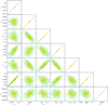 |
Fig. A.1 Scatter plot of points in the MCMC chain for the 2L1S model. Colors are set to represent points within 1σ (red), 2σ (yellow), 3σ (green), 4σ (cyan), and 5σ (blue). |
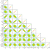 |
Fig. A.2 Scatter plot of MCMC chain points for the 3L1S model. Colors of points are same as those in Fig. A.1. |
References
- Albrow, M. 2017, https://doi.org/10.5281/zenodo.268049 [Google Scholar]
- Albrow, M. D., Beaulieu, J.-P., Caldwell, J. A. R., et al. 2000, ApJ, 534, 894 [NASA ADS] [CrossRef] [Google Scholar]
- Bennett, D. P., Rhie, S. H., Udalski, A., et al. 2016, AJ, 152, 125 [Google Scholar]
- Bennett, D. P., Udalski, A., Han, C., et al. 2018, AJ, 155, 141 [Google Scholar]
- Bennett, D. P., Udalski, A., Bond, I. A., et al. 2020, AJ, 160, 72 [NASA ADS] [CrossRef] [Google Scholar]
- Bensby, T. Yee, J. C., Feltzing, S., et al. 2013, A&A, 549, A147 [NASA ADS] [CrossRef] [EDP Sciences] [Google Scholar]
- Bessell, M. S., & Brett, J. M. 1988, PASP, 100, 1134 [Google Scholar]
- Danek, K., & Heyrovský, D. 2015, ApJ, 806, 99 [CrossRef] [Google Scholar]
- Danek, K., & Heyrovský, D. 2019, ApJ, 880, 72 [CrossRef] [Google Scholar]
- Fischer, D. A., Butler, R. P., Marcy, G. W., Vogt, S. S., & Henry, G. W. 2003, ApJ, 590, 1081 [NASA ADS] [CrossRef] [Google Scholar]
- Gaudi, B. S., Bennett, D. P., Udalski, A., et al. 2008, Science, 319, 927 [Google Scholar]
- Gould, A. 1992, ApJ, 392, 442 [Google Scholar]
- Gould, A., Udalski, A., Shin, I.-G., et al. 2014, Science, 345, 46 [Google Scholar]
- Grieger B., K. R., Refsdal S., & Stabell R. 1989 Abhandlungen aus der Hamburger Sternwarte, 10, 177 [Google Scholar]
- Han, C. 2006, ApJ, 638, 1080 [Google Scholar]
- Han, C. 2008, ApJ, 676, L53 [Google Scholar]
- Han, C., Chang, H.-Y., & An, J. H. 2001, MNRAS, 328, 986 [NASA ADS] [CrossRef] [Google Scholar]
- Han, C., Bennett, D. P., Udalski, A., & Jung, Y. K. 2016, ApJ, 825, 8 [NASA ADS] [CrossRef] [Google Scholar]
- Han, C., Udalski, A., Gould, A., et al. 2017, AJ, 154, 223 [Google Scholar]
- Han, C., Lee, C.-U., Udalski, A., et al. 2020, AJ, 159, 48 [Google Scholar]
- Han, C., Albrow, M. D., Chung, S.-J., et al. 2021a, A&A, 652, A145 [NASA ADS] [CrossRef] [EDP Sciences] [Google Scholar]
- Han, C., Lee, C.-U., Ryu, Y.-H., et al. 2021b, A&A, 649, A91 [NASA ADS] [CrossRef] [EDP Sciences] [Google Scholar]
- Han, C., Gould, A., Kim, D., et al. 2022, A&A, 663, A145 [NASA ADS] [CrossRef] [EDP Sciences] [Google Scholar]
- Han, C., Udalski, A., Jung, Y. K., et al. 2023, A&A, 670, A172 [NASA ADS] [CrossRef] [EDP Sciences] [Google Scholar]
- Han, C., Udalski, A., Jung, Y. K., et al. 2024, A&A, 685, A16 [NASA ADS] [CrossRef] [EDP Sciences] [Google Scholar]
- Jung, Y. K., Udalski, A., Bond, I. A., et al. 2017, ApJ, 841, 75 [Google Scholar]
- Jung, Y. K., Udalski, A., Gould, A., et al. 2018, AJ, 155, 219 [Google Scholar]
- Jung, Y. K., Han, C., Udalski, A., et al. 2021, AJ, 161, 293 [NASA ADS] [CrossRef] [Google Scholar]
- Kervella, P., Thévenin, F., Di Folco, E., & Ségransan, D. 2004, A&A, 426, 29 [Google Scholar]
- Kim, S.-L., Lee, C.-U., Park, B.-G., et al. 2016, JKAS, 49, 37 [Google Scholar]
- Mugrauer, M., Seifahrt, A., Neuhüser, R., & Mazeh, T. 2006, MNRAS, 373, L3 [Google Scholar]
- Nakajima, T., Oppenheimer, B. R., Kulkarni, S. R., Matthews, K., & Golimowski, D. A. 1995, Nature, 378, 463 [NASA ADS] [CrossRef] [Google Scholar]
- Nataf, D. M., Gould, A., Fouqué, P., et al. 2013, ApJ, 769, 88 [Google Scholar]
- Poleski, R., Skowron, J., Udalski, A., et al. 2014, ApJ, 795, 42 [Google Scholar]
- Rattenbury, N. J., Mao, S., Sumi, T., & Smith, M. C. 2007, MNRAS, 378, 1064 [NASA ADS] [CrossRef] [Google Scholar]
- Rhie, S. H. 2002, arXive-prints [arXiv:astro-ph/0202294] [Google Scholar]
- Todorov, K., Luhman, K. L., & McLeod, K. K. 2010, ApJ, 714, L84 [NASA ADS] [CrossRef] [Google Scholar]
- Tuomi, M., Jones, Hugh R. A., Barnes, J. R., Anglada-Escudë, G., & Jenkins, J. S. 2014, MNRAS, 441, 1545 [NASA ADS] [CrossRef] [Google Scholar]
- Udalski, A. 2003, AcA, 53, 291 [NASA ADS] [Google Scholar]
- Udalski, A., Szymanski, M. K., & Szymanski, G. 2015a, AcA, 65, 1 [Google Scholar]
- Udalski, A., Jung, Y. K., Han, C., et al. 2015b, ApJ, 812, 47 [NASA ADS] [CrossRef] [Google Scholar]
- Yang, H., Yee, J. C., Hwang, K.-H., et al. 2024, MNRAS, 528, 11 [NASA ADS] [CrossRef] [Google Scholar]
- Yee, J. C., Shvartzvald, Y., Gal-Yam, A., et al. 2012, ApJ, 755, 102 [Google Scholar]
- Yoo, J., DePoy, D. L., Gal-Yam, A., et al. 2004, ApJ, 603, 139 [Google Scholar]
- Zang, W., Han, C., Kondo, I., et al. 2021, RAA, 21, 239 [NASA ADS] [Google Scholar]
- Zhang, K., Zang, W., El-Badry, K., et al. 2024, Nat. Astron., 8, 1575 [Google Scholar]
- Zucker, S., Mazeh, T., Santos, N. C., Udry, S., & Mayor, M. 2003, A&A, 404, 775 [NASA ADS] [CrossRef] [EDP Sciences] [Google Scholar]
- Zucker, S., Mazeh, T., Santos, N. C., Udry, S., & Mayor, M. 2004, A&A, 426, 695 [NASA ADS] [CrossRef] [EDP Sciences] [Google Scholar]
All Tables
All Figures
|
Fig. 1 Light curve of the lensing event KMT-2024-BLG-0404. The lower panel presents the overall view, while the upper panel provides a close-up of the caustic-crossing features. The curve overlaid on the data points represents the best-fit 2L1S model, which was derived by excluding data from the interval 407.5 < HJD′ < 408.0. In the lower panel, arrows labeled t1, t2, t3, t4, and t5 mark the positions of specific anomaly features. |
| In the text | |
|
Fig. 2 Lens system configuration corresponding to the best-fit 2L1S model. The cuspy closed red figure represents the caustic, while the two blue dots labeled M1 and M2 denote the positions of the binary-lens components. The arrowed line illustrates the trajectory of the source. The four empty circles, scaled to the source size, mark the source positions along its trajectory at the times corresponding to the anomaly features at t1, t2, t4, and t5. The gray curves surrounding the caustic represent the equi-magnification contours. |
| In the text | |
|
Fig. 3 Map of Δχ2 on the log s3–log q3 parameter surface derived from the triple-lens modeling. The color coding indicates points with Δχ2 ≤ 1nσ (red), ≤ 2nσ (yellow), ≤ 3nσ (green), ≤ 4nσ (cyan), and ≤ 5nσ (blue), where n = 4. |
| In the text | |
|
Fig. 4 Comparison of the models (2L1S, 2L2S, and 3L1S) in the region around caustic spikes. The lower panels show the residuals from the models. |
| In the text | |
|
Fig. 5 Lens system configuration for the 3L1S model. The notations are the same as in Fig. 2. The inset presents a close-up of the area surrounding the planet-induced caustics. In comparison to the configuration shown in Fig. 2, the position of the third lens component (M3) and the source position at time t3 are additionally indicated. |
| In the text | |
|
Fig. 6 Positions of the source and the centroid of the RGC in the instrumental CMD of stars lying near the source. |
| In the text | |
|
Fig. 7 Bayesian posteriors for the mass of the heaviest lens component (M2), distances to the lens and source (DL and DS). In each distribution, the solid vertical line represents the median value, while the 1σ uncertainty range is indicated by two dotted lines. The curves shown in blue and red represent the contributions from the disk and bulge lens populations, respectively, while the black line denotes the combined contribution of both populations. |
| In the text | |
|
Fig. A.1 Scatter plot of points in the MCMC chain for the 2L1S model. Colors are set to represent points within 1σ (red), 2σ (yellow), 3σ (green), 4σ (cyan), and 5σ (blue). |
| In the text | |
|
Fig. A.2 Scatter plot of MCMC chain points for the 3L1S model. Colors of points are same as those in Fig. A.1. |
| In the text | |
Current usage metrics show cumulative count of Article Views (full-text article views including HTML views, PDF and ePub downloads, according to the available data) and Abstracts Views on Vision4Press platform.
Data correspond to usage on the plateform after 2015. The current usage metrics is available 48-96 hours after online publication and is updated daily on week days.
Initial download of the metrics may take a while.