| Issue |
A&A
Volume 700, August 2025
|
|
|---|---|---|
| Article Number | A135 | |
| Number of page(s) | 16 | |
| Section | Extragalactic astronomy | |
| DOI | https://doi.org/10.1051/0004-6361/202453027 | |
| Published online | 13 August 2025 | |
Reconciling PTA and JWST, and preparing for LISA with POMPOCO: a Parametrisation Of the Massive black hole POpulation for Comparison to Observations
1
Max Planck Institute for Gravitationsphysik (Albert Einstein Institute), Am Mühlenberg 1, 14476 Potsdam, Germany
2
Dipartimento di Fisica “G. Occhialini”, Università degli Studi di Milano-Bicocca, Piazza della Scienza 3, 20126 Milano, Italy
3
INFN, Sezione di Milano-Bicocca, Piazza della Scienza 3, 20126 Milano, Italy
4
School of Mathematical Sciences, University of Nottingham, University Park, Nottingham NG7 2RD, United Kingdom
5
Institut d’Astrophysique de Paris, UMR 7095, CNRS and Sorbonne Université, 98 bis Boulevard Arago, 75014 Paris, France
6
SISSA – Scuola Internazionale Superiore di Studi Avanzati, Via Bonomea 265, 34136 Trieste, Italy
7
INFN Sezione di Trieste, via Valerio 2, 34127 Trieste, Italy
8
IFPU – Institute for Fundamental Physics of the Universe, Via Beirut 2, 34014 Trieste, Italy
9
Université Paris Cité, CNRS, Astroparticule et Cosmologie, F-75013 Paris, France
10
Department of Astrophysical Sciences, Princeton University, Princeton, NJ 08544, USA
⋆ Corresponding author.
Received:
15
November
2024
Accepted:
23
June
2025
Abstract
Aims. We develop a parametrised model to describe the formation and evolution of massive black holes. This model is designed for comparisons with observations of electromagnetic and gravitational waves.
Methods. Using an extended Press-Schechter formalism, we generated dark matter halo merger trees. We then seeded and evolved massive black holes through parametrised prescriptions. This approach avoids solving differential equations and is computationally efficient. It enabled us to analyse observational data and infer the parameters of our model in a fully Bayesian framework.
Results. Observations of the black hole luminosity function are compatible with the nanohertz gravitational-wave signal (that is likely) measured by pulsar-timing arrays when we allow for a higher luminosity function at high redshift (4 − 7), as was recently suggested based on observations with the James Webb Space Telescope. Our model can simultaneously reproduce the bulk of the M* − MBH relation at z − 0 and its outliers. Cosmological simulations struggle to do this. The inferred model parameters are consistent with expectations from observations and more complex simulations: They favour heavier black hole seeds and short delays between halo and black hole mergers while requiring super-Eddington accretion episodes that last a few dozen million years, which in our model are linked to galaxy mergers. Accretion is suppressed in the most massive black holes below z ≃ 2.5 in our model, which is consistent with the anti-hierarchical growth hypothesis. Finally, our predictions for LISA, although fairly broad, agree with previous models that assumed an efficient merging of massive black holes that formed from heavy seeds.
Conclusions. Our model offers a new perspective on the apparent tensions between the black hole luminosity function and the latest results from the James Webb Space Telescope and pulsar-timing arrays. Its flexibility makes it ideal to fully exploit the potential of future gravitational-wave observations of massive black hole binaries with LISA.
Key words: galaxies: evolution / galaxies: luminosity function / mass function / quasars: supermassive black holes
© The Authors 2025
 Open Access article, published by EDP Sciences, under the terms of the Creative Commons Attribution License (https://creativecommons.org/licenses/by/4.0), which permits unrestricted use, distribution, and reproduction in any medium, provided the original work is properly cited.
This article is published in open access under the Subscribe to Open model.
Open access funding provided by Max Planck Society.
1. Introduction
Massive black holes (MBHs) with masses of 105 − 109 M⊙ reside at the centre of most galaxies in our local Universe (Gehren et al. 1984; Kormendy & Richstone 1995; Reines et al. 2011, 2013; Baldassare et al. 2020), including in our own Milky Way. These cosmic giants play a crucial role in the evolution and dynamics of galaxies, as was demonstrated by numerous scaling relations between the properties of galaxies and their MBHs (Ferrarese & Merritt 2000; Tremaine et al. 2002; Kormendy & Ho 2013; McConnell & Ma 2013; Schramm & Silverman 2013; Scott et al. 2013; Shankar 2013; Shankar et al. 2020; Sahu et al. 2019; Greene et al. 2020), such as the M* − MBH relation with the stellar mass of the host galaxy. These linked properties indicate that MBHs track the hierarchical formation of galaxies, and they might indicate that MBHs and galaxies mutually affect each other. The details of the processes governing the origin, growth, activity, and feedback of these black holes (BHs) remain highly debated, however.
The general scenario is as follows. MBHs must have originated at high redshift from lighter black hole seeds. Several seed models have been proposed that ranging from “light” to “heavy” masses (for a review, see Latif & Ferrara 2016; Volonteri et al. 2021). At the largest scales, the fate of a seed is determined by the evolution of its host dark matter (DM) halo, which proceeds hierarchically in mass. Within the host galaxy, the growth of the seed proceeds primarily through the accretion of gas (Yu & Tremaine 2002) and in a minor part via the accretion of stars (Rees 1988), with periods of intense accretion activity likely alternating with quiescent phases. Intense accretion emits significant energy in a variety of forms: Radiation is emitted across the electromagnetic spectrum (Fabian 2012), while kinetic and thermal energy can affect the gas temperature, density, and turbulence, and it can in turn prevent new gas from reaching the MBH and temporarily suppress the process (AGN feedback). To a lesser extent (Ricarte et al. 2019), BH mergers following the merger of their host galaxies can also contribute to the growth of MBHs (Dubois et al. 2014a; Kulier et al. 2015).
One of our best probes of the population of MBHs is the luminosity function (LF) of accreting MBHs: quasars and active galactic nuclei (AGNs) more generally. This has been the target of surveys in the X-ray, UV, optical, infrared, and radio bands (see Hopkins et al. 2007; Shen et al. 2020, and references therein). These surveys cover distances of up to z ≲ 7 and revealed that the LF evolves strongly with redshift in normalisation and shape. Interestingly, mid-infrared surveys appeared to differ from these results. Using observations from the Spitzer Space Telescope survey (Werner et al. 2004), Lacy et al. (2015) found an increased LF up to z ∼ 3. The higher-redshift mid-infrared Universe is now being probed by the James Webb Space Telescope (JWST) (Gardner et al. 2006). It has detected dozens of candidate AGNs at high redshift (z ∼ 4 − 11), including some at lower bolometric luminosities than were observed before (Lbol ∼ 1044 − 1046 erg/s) (e.g. Onoue et al. 2023; Kocevski et al. 2023; Maiolino et al. 2024; Übler et al. 2023; Kokorev et al. 2023; Lyu et al. 2024). The first results for the LF and mass function derived from these observations (Harikane et al. 2023; Maiolino et al. 2024; Greene et al. 2024; Matthee et al. 2024; Taylor et al. 2025) also indicate an increased LF compared to previous expectations based on the compilation of data from mid-IR to X-ray, but dominated at high redshift by X-ray and UV observations (Shen et al. 2020). It has been suggested that the masses and abundance of (candidate) MBHs found by the JWST at very high redshifts might pose a challenge for lighter seed scenarios and might require continuous and intense accretion even for heavier seeds (e.g. Harikane et al. 2023; Maiolino et al. 2024; Kokorev et al. 2023; Greene et al. 2024). At the same time, the models that produce the heaviest seeds appear to struggle to produce enough seeds to explain the abundance of (candidate) MBHs (Regan & Volonteri 2024) (see also Habouzit 2024 for a discussion of the compatibility of different simulations of MBH evolution with these results).
These electromagnetic observations are now being complemented with gravitational-wave (GW) observations because pulsar-timing array (PTA) collaborations are likely close to confirming the detection of a stochastic background consistent with merging MBH binaries with masses ≳108 M⊙ (Antoniadis et al. 2023a; Agazie et al. 2023a; Tarafdar et al. 2022; Reardon et al. 2023; Xu et al. 2023). It is generally thought that the preliminary result for the PTA background, with its relatively high amplitude, would require MBHs to merge and accrete efficiently (Agazie et al. 2023b; Antoniadis et al. 2024a; Barausse et al. 2023; Izquierdo-Villalba et al. 2024) (although see Goncharov et al. 2024). In the next decade, the Laser Interferometer Space Antenna (LISA) will further extend our understanding of merging MBHs by detecting GWs from binaries with lower masses (104 − 108 M⊙) and up to very high redshifts (z ∼ 20) (Amaro-Seoane et al. 2017; Colpi et al. 2024).
The astrophysical interpretation of observations is achieved by a comparison to theoretical models for the formation and evolution of MBHs. Cosmological N-body and hydrodynamic simulations have become valuable tools for simulating MBHs through the increased computational power and more accurate sub-grid models for MBH accretion, seeding, feedback, and dynamics (see, e.g. Volonteri et al. 2016; Springel et al. 2017; Kannan et al. 2021; Ni et al. 2022; Bhowmick et al. 2024). In addition, semi-analytical models (SAMs; e.g. Cole et al. 2002; Volonteri et al. 2003; Monaco et al. 2007; Somerville et al. 2008; Benson 2012; Barausse 2012; Ricarte & Natarajan 2018; Bonetti et al. 2019; Dayal et al. 2019; Izquierdo-Villalba et al. 2020; Barausse et al. 2020; Trinca et al. 2022) have been widely used to simulate the cosmic history of MBHs because their computational cost is lower. A computationally cheaper alternative to both SAMs and cosmological simulations are empirical models (see, e.g. Soltan 1982; Small & Blandford 1992; Tucci & Volonteri 2017; Conroy & White 2012; Allevato et al. 2021). Instead of making physical assumptions, these models use observations to empirically (and self-consistently) characterise the evolution of MBHs. Empirical models have grown increasingly more complex, and some (Zhang et al. 2023; Boettner et al. 2025) encompass DM haloes, galaxies, and MBHs and count about 50 parameters. The more complex the model, the greater the number observations that must be used to constrain its parameters, from scaling relations to luminosity and mass functions.
Cosmological simulations and SAMs are too computationally expensive to compare the full range of alternative models and parameter space with observations. This results in a set of discrete models. This is a major obstacle for astrophysical inference within a Bayesian framework. In Toubiana et al. (2021), some of the authors of this paper studied mock LISA data and showed that inference with a finite set of discrete population models could lead to severe biases in the underlying astrophysical parameters. Empirical models, while sufficiently fast for a Bayesian parameter estimation (see, e.g. Zhang et al. 2023; Boettner et al. 2025), focus on statistical and empirical properties and not on the underlying physics.
The goal of this work is to provide a fast parametric approach to infer the physics behind the evolution of MBHs from current observations, and prepare for the LISA mission. We introduce our model POMPOCO, which stands for Parametrisation Of the Massive black hole POpulation for Comparison to Observations. It adopts an approach that is intermediate between SAMs and empirical models by proposing an effective description of the formation and evolution of MBHs within their host haloes. As a first application of POMPOCO, we jointly fit the LF at low and high redshifts and the amplitude of the GW background measured by PTA using a Markov chain Monte Carlo (MCMC) algorithm to determine the parameter sets that are compatible with the desired datasets. We validate our results on the M* − MBH relation at z = 0 and at higher redshift, for which we do not explicitly fit. The results agree well with the proposed fit of Greene et al. (2020). Finally, we compute predictions for LISA conditioned on these observations.
This paper is organised as follows. Section 2 describes our parametric model. In Sects. 3 and 4, we construct observables from our model and use them to fit the model parameters to observations. We present our results in Sect. 5 and make predictions for the LISA mission in Sect. 6. We summarise and conclude in Sect. 7. In the remainder of the paper, MBH masses are defined in the source frame.
2. Description of the model
We describe the components of our model below. We also summarise all the parameters and the settings of our model in Table 1. In general, our choice of prescriptions is guided by a combination of physical, observational, and simulation-based considerations, as well as a deliberate effort to maintain flexibility and allow the data to inform the inference. In the current version of our model, we do not track the evolution of the spins of MBHs. We hope to do so in future work.
Parameters and settings of our model.
We adopt a flat ΛCDM cosmology with H0 = 67.77 km s−1 Mpc−1, Ωm = 0.3071, Ωb = 0.04820 and δc, 0 = 1.686 for the critical overdensity for spherical collapse at z = 0. Given the tight constraints on cosmological parameters, we expect the uncertainty from cosmology to be small compared to the astrophysical uncertainty.
2.1. Dark matter halo merger tree
We generated DM halo merger trees down to zmax = 20 using the implementation of the extended Press-Schechter formalism (Press & Schechter 1974; Bond et al. 1991; Bower 1991; Lacey & Cole 1993) described in Appendix A of Parkinson et al. (2008). We used updated values given in Benson (2017) for the phenomenological modifications to the original extended Press-Schechter formalism, introduced to better reproduce cosmological simulations. We used a time-varying mass resolution, as proposed in Volonteri et al. (2003): Mh, res = 10−3Mh, 0(1 + z)−3.5, where Mh, 0 is the mass of the halo at z = 0.
The suite of trees was built drawing the halo masses at z = 0 from a log-uniform distribution. Each tree entered the calculation of population properties by reweighting the BHs in that tree by their Press-Schechter weight.
2.2. Massive black hole seeds
We populated leaf haloes – the last haloes along the branches of the merger trees1 – with seed BHs. We only seeded haloes at z ≥ 10 and with mass above a threshold Mh, seed, with probability fseed.
The nature and mass spectrum of the original seeds of the observed population of MBHs is currently unconstrained. Proposed seeding mechanisms range from light seeds (below 103 M⊙), resulting from the first stars or formed primordially, and heavy seeds (between 103 M⊙ and 106 M⊙) resulting from runaway accretion, mergers or supermassive stars. For a recent review of these mechanisms, which are not mutually exclusive, see Volonteri et al. (2021). We allowed our model to probe the seed distribution by drawing the mass of the seed BH from a truncated log-normal distribution, with mean μseed and standard deviation σseed. The log-normal distribution is meant to capture a single formation scenario, characterised by a range of seed masses around a central value. At the high end, we limited the mass of the BH seed to 10% of the baryonic mass of the halo MhΩb/(Ωm − Ωb). At the low end, we took the minimum seed mass to be 100 M⊙2. We denoted the seeded BH as the primary BH of the DM halo.
2.3. Halo and massive black hole mergers
Following the merger of two haloes, we tracked the evolution of the BHs they contain, distinguishing between major and minor halo mergers, based on the halo mass ratio qh = Mh, 2/Mh, 1 ≤ 1. Based on the results of our simulations, we set the threshold for major mergers to qh, major = 0.13, which is similar to the value used in Ricarte & Natarajan (2018).
2.3.1. Formation of black hole binaries
Following major mergers, where qh ≥ qh, major, we checked whether either halo hosts a BH. If there was only one BH, this became the primary BH of the newly formed halo. If there was one BH in each, they formed a binary with merger time given by the sum of the dynamical friction (DF) timescale and additional delays (see Sect. 2.3.3). Finally, if there were more BHs, we use the prescription for multiple interactions described below.
In the case of minor mergers, BHs in the lighter halo had to sink into the heavier halo before being counted as primary BH or forming a binary. The BHs of the lighter halo were therefore dubbed as outer BHs of the heavier halo. The sinking time is given by the DF timescale of the satellite halo into the primary one. If the lighter halo contained a binary that merges before the sinking time, we allowed it to merge and assign the merger product to the new halo as an outer BH. We retained (the most massive) half of the outer BHs of the lighter halo, in addition to its potential primary/binary, up to a limit of four outer BHs. We found that this is an acceptable limitation, as small BHs in small haloes play a minor role. Similarly, following major mergers, we retained up to four of the outer BHs of the two haloes, selecting the ones with the shorter sinking times. When outer BHs sunk into the centre of the halo, they either became the primary BH of that halo if it contained none, or formed a binary that merged within tdelay (see Sect. 2.3.3). If the halo already contained a binary, or multiple outer BHs sunk within one time step, we used our prescription for multiple interactions described in Sect. 2.3.2.
2.3.2. Multiple interactions
We used the results of Bonetti et al. (2018a) to handle interactions between more than two BHs. Bonetti et al. (2018a) explored the outcome of three-body interactions between MBHs accounting for relativistic corrections to the Newtonian equations of motion. They found that, on average, there is a probability pmulti = 0.22 (see their Table 2) that the interaction of an MBH binary with a third MBH will lead to a rapid merger (within a few hundred million years), usually between the two most massive MBHs. In the remaining cases, the MBH binary is little affected by the third MBH. Based on these results, we decided with probability pmulti = 0.22 if the BHs undergo a multiple interaction or not. If it occurred, we retained the two most massive BHs and drew the merger time (in yr) from a log-normal distribution with mean 8.4 dex and standard deviation 0.4 dex (see Fig. 7 of Bonetti et al. 2018a). If they did not undergo a multiple interaction, we distinguished between two cases, depending on how the BHs met. If there was a binary and a third BH was brought either by a halo merger or by an outer BH that sunk, we kept the original binary, and its time to merger was unaffected. If there was no binary originally, for instance, if there was a primary BH and two outer BHs sunk within one time step, we just kept the two most massive among them, and formed a binary merging within tdelay (see Sect. 2.3.3). In any case, we did not keep track of the other BHs.
2.3.3. Dynamical friction and other delays
Satellite haloes (and their BHs) sink to the centre of the primary halo via DF, whose typical timescale is set by (Lacey & Cole 1993; Binney & Tremaine 1987)
 (1)
(1)
 (2)
(2)
 (3)
(3)
where we made the same choice for the numerical prefactor as in Volonteri et al. (2003)3, and where H(z) is the Hubble factor at the desired redshift. We neglected any possible variations in the DF timescale due to the initial conditions of the infall, and effects such as tidal stripping and tidal heating of the satellite halo.
Once the satellite halo has sunk into the primary one, the two galaxies they host will merge thanks to additional DF. The BHs at their centre will then form a bound binary, with separation of order of a parsec. The binary will undergo several other processes that affect its orbital decay, including stellar hardening and interactions with nuclear gas (see Colpi 2014, for a review). We modelled these additional delays with a single parameter, tdelay, taken to be the same for all binaries. Our model could be extended by allowing the delay time to be drawn from a parametrised distribution that depends on the physical parameters of the system.
2.3.4. Merger
Once the total time delay had elapsed, binaries merged and formed remnants with mass given by the sum of the masses at the time of the merger. We neglected the mass loss due to the emission of GWs, but we did account for the accretion occurring from binary formation until merger, using the prescriptions described in the section below. We labelled the merger remnant as the primary BH of its host halo.
We did not model kicks on the remnant BH due to the emission of GWs, which could displace the BH from the centre of its host, because they depend sensitively on the BH spins and the details of the orbit at the time of merger (eccentricity, spin inclinations), which we did not track in the current version of POMPOCO. Kicks are expected to have a small impact in high-mass galaxies, because of their large escape velocity. Those are the galaxies that contribute the most to the GW background in the nHz band and the high end of the LF, which are the observables of interest for this paper. Neglecting kicks is therefore expected to have little impact on our results. It might impact the LISA rates, however, because many LISA mergers occur in low-mass galaxies, and could modify the low mass end of the M* − MBH relation. We left the inclusion of kicks for future work.
2.4. Accretion
We parametrised the growth of the mass of a BH, mBH, through accretion by the Eddington ratio, fEdd,
 (4)
(4)
 (5)
(5)
 (6)
(6)
where ṁEdd and LEdd are the Eddington accretion rate and luminosity, respectively, ϵ is the radiative efficiency, and tEdd = 450 Myr defines the accretion timescale. In this way, the mass between two time steps increases as
 (7)
(7)
We took the radiative efficiency to be 0.1. Inspired by Ricarte & Natarajan (2018), we considered two accretion modes: burst and steady accretion.
The burst mode was triggered following a major halo merger, qh ≥ qh, major. Such mergers are expected to feed the reservoir surrounding MBHs, leading to an episode of intense accretion. When this happened, the most massive BH in the resulting galaxy started accreting for a time tburst with an Eddington ratio fEdd, burst. In the burst mode, we did allow for super-Eddington accretion, and drew fEdd, burst from a power-law distribution with slope (γburst − 1) < 0 between 10−2 and 10. In this work, we considered a common burst time tburst for all BHs. If the resulting halo underwent another major merger before a time tburst had elapsed, we restarted the count. The choice of a power-law distribution with negative slope is motivated by the general expectation that super-Eddington accretion should be rare. Aird et al. (2018) found that X-ray observations of AGN activity across redshift and galaxy type suggest a steep power-law at high accretion rates, allowing for rare and short-lived periods of super-Eddington accretion.
Whenever they were not accreting in the burst mode, BHs accreted in the steady mode with an Eddington ratio fEdd, steady drawn from a log-normal distribution with mean μsteady and variance σsteady truncated at the high end at 1. When drawing fEdd, steady, we drew jointly tsteady from a log-uniform distribution between 1 and 100 Myr. After a time tsteady had elapsed, we drew again both quantities. This procedure is meant to capture the variability of AGNs. The choice of a log-normal distribution is motivated by Volonteri et al. (2016), Fig. 14, which shows the distribution of accretion rates in AGNs from the Horizon-AGN simulation (Dubois et al. 2014b). Observations also suggest that accretion rates could follow a combination of log-normal and power law distributions, see Aird et al. (2018).
The most massive BHs are observed to be quiescent at low redshift due to gas having been consumed by star formation, as well as affected by supernova and AGN feedback (see Merloni 2004; Hirschmann et al. 2012, 2014, and references therein). To reproduce this, for z ≤ zcut we shut off accretion for BHs with mMBH ≥ mcut(z). We parametrised mcut(z) as
 (8)
(8)
where log10mcut, 0 and αcut are parameters of our model, together with zcut. We imposed αcut ≥ 0 so that the mass cut is larger at higher redshift. This approach gives our model the flexibility to capture the anti-hierarchical growth observed in data and simulations (Merloni 2004; Hirschmann et al. 2012, 2014), without enforcing it a priori4.
We applied the prescriptions above to the primary and binary BHs of all haloes. Outer BHs do not accrete in our model, as we do not expect them to have a sufficient reservoir to accrete significantly. Both BHs in a binary had the same fEdd (either burst or steady).
3. Observables
In order to compare our model with observations we generated full MBH population for different choices of parameters. To do so, we applied the following procedure:
-
We built Nh merger trees, drawing the mass of the haloes at z = 0 from a log-normal distribution between 1011 and 1015 M⊙;
-
We populated each merger tree according to the model parameters;
-
We saved the properties of the BHs in the merger tree (mass, Eddington ratio, mass of the host halo, etc.) at a set of redshifts.
In this work, we generated Nh = 2000 haloes.
The generation of the DM halo merger tree is the most time-consuming step of our model. Fortunately, none of the parameters affect this step. We could therefore generate a single merger tree and run simulations for many sets of parameters on it. This resulted in a relatively fast model, and allowed us to thoroughly explore the parameter space. As an example, it takes ∼1 hour to generate a merger tree and run the simulation for 500 sets of parameters on it. The 2000 merger trees were run in parallel and the results were combined in post-processing.
We will now describe how we transformed the output of our simulations into quantities that can be compared with observations: the LF, the stellar mass-black hole mass relation, the stochastic GW background, and the merger rate.
3.1. Luminosity function
The luminosity of a BH is given by
 (9)
(9)
where fEdd is either the burst mode or steady mode Eddington ratio, depending on the current accretion mode of the BH. We assigned binaries a luminosity equal to the sum of the luminosities of the individual BHs (recall that in our model, BHs in a binary share the same fEdd). Outer BHs of a halo were not included in the computation of the LF since we do not expect them to accrete significantly.
We denote the LF at redshift z0 by Φ(LBH, z0). It is given by the weighted sum of the contribution from each halo merger tree,
 (10)
(10)
where WPS(Mh, 0) is the Press-Schechter weight for a halo of mass Mh, 0 at z = 0 and  is the number of BHs with luminosity LBH at redshift z0 in the merger history of a halo of mass Mh, 0 at z = 0. We computed the integral in a discrete way, by the PS-weighted sum of the individuals histograms of each tree. Binning in log-luminosity, we have for the LF in bin k
 (11)
(11)
with ΔLBH the size of the bin in log10LBH and 𝒟h = log10(Mh, 0, max)−log10(Mh, 0, min) coming from the normalisation of the log-uniform distribution used to draw the halo masses. The Poisson error in each bin is obtained by assuming that the histograms resulting from the different simulations are independent Poisson realisations. The variances thus sum up and the error is given by
 (12)
(12)
3.2. Relation of the stellar mass to the black hole mass
In our code, we did not directly model the evolution of the stellar mass M* of a given halo. Instead, we used the halo mass-stellar mass relation of Moster et al. (2010) to convert Mh into M*, including the scatter in the relation, to account for the spread in the relation. We also accounted for the redshfit evolution of the relation when computing the M* − MBH relation at high z.
For a given stellar mass at redshift z0, we can compute the average black hole mass across haloes at that redshift as
 (13)
(13)
where  is the number of haloes at redshift z0 that contain a BH with mass mBH and whose stellar mass is M*, in the merger history of a halo of mass Mh, 0 at z = 0.
In practice, we predefined a fixed binning scheme for the stellar masses, and then associated each halo hosting a BH to the corresponding M*, k bin based on the Mh − M* relation of Moster et al. (2010). We have
 (14)
(14)
where mBH, i, j, k are the masses of the BHs in haloes at z0 in the i-th simulation whose stellar mass is in the M*, k bin, and Ni, k is the number of such haloes. In the case of binaries, we used the total mass. Outer BHs are not included in this computation.
We computed the standard deviation of the MBH − M* relation as
 (15)
(15)
Technically, there should also be a Poisson error (on Ni), but we neglected it, as we take the bins in stellar mass to be big enough so that the dominant source of error is the variance of BH masses within that bin and not the counting.
3.3. Stochastic gravitational-wave background
We computed the stochastic GW signal in the PTA band of our simulations with the formalism of Phinney (2001) and Sesana et al. (2008). In this work, we assumed binaries to be on quasi-circular orbits. We introduced the chirp mass of a binary with masses m1 and m2 as ℳc = (m13m23)/(m1 + m2)5. Denoting the characteristic GW amplitude at (observer) frequency f as hc(f), we have
 (16)
(16)
where  is the number of haloes hosting a binary merger with chirp mass ℳc at redshift z in the merger history of a halo of mass Mh, 0 at z = 0, and
  is the energy emitted in the source rest-frame at frequency fr = f(1 + z). For quasi-circular binaries, the latter is given by
 (17)
(17)
The characteristic strain thus has a power-law frequency dependence
 (18)
(18)
The amplitude is determined here by the distribution of mergers in a given simulation. In practice, we performed a Monte Carlo integration,
 (19)
(19)
where the second sum is performed over all the mergers in the i-th merger tree. The Poisson error is then given by
 (20)
(20)
Finally, following Antoniadis et al. (2024a), we define the root-mean-square residual as
 (21)
(21)
where Δf is the frequency resolution (the inverse of the observation time).
3.4. Merger rate
We introduce mt = m1 + m2 as the total mass of an MBH binary and qb = m1/m2 ≥ 1 its mass ratio. The rate of MBH mergers per unit mt, qb and z is computed as
 (22)
(22)
where dc(z) is the comoving distance at redshift z and  is the number of MBH mergers with parameters (mt, qb, z) in the merger history of a halo of mass Mh, 0 at z = 0, t is the detector-frame time. Monte Carlo integration gives
 (23)
(23)
In practice, to generate samples of observed MBH merger events for an observation time Tobs we used the following procedure. We read the (mt, qb, z) values of all merger events in our trees, attributed them a Poisson rate
 (24)
(24)
and drew the number of such events from a Poisson distribution with expected number λ(mt, qb, z)Tobs.
The detector-frame rate as a function of a single parameter, for example mt, was obtained by marginalising over the remaining parameters, and the total rate was obtained by marginalising over all parameters (mt, qb, z)
 (25)
(25)
see also Eq. (2) of Hartwig (2019). Finally, Monte Carlo integration gives
 (26)
(26)
4. Fitting to observations
As a first application of POMPOCO, we fitted jointly the LF across redshifts and the GW stochastic background.
4.1. Observations
As the observed LF, we considered a combination of the fits from Lacy et al. (2015) (fit: ‘All’) and Shen et al. (2020) (fit: ‘global A’), as described in the next section (Fig. 1). The fit by Shen et al. (2020) is based on a wide range of observations in the rest-frame mid-IR, B band, UV, soft and hard X-ray going up to z ∼ 7. The constraint by Lacy et al. (2015) is only based on the mid-IR Spitzer Space Telescope survey with observations up to z ∼ 3. It is also included in the compilation of Shen et al. (2020), although the latter is mainly driven by the more abundant B, UV, and X-ray data. The mid-IR LF fit in Lacy et al. (2015), if taken alone, suggests more AGN at a given bolometric luminosity. We further extrapolated the Lacy et al. (2015) fit to higher redshifts and lower luminosities than covered by their data.
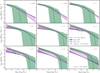 |
Fig. 1. Evolution of the luminosity function. In green, we show the prediction of our model when fitting for the LF itself at redshifts 0.25, 0.5, 3 and 6, as well as for the GW background measured by EPTA, displaying the median (green line) and 90% confidence interval (green band). This should be compared with the fits to the observed LF from Lacy et al. (2015) (pink) and Shen et al. (2020) (purple) and the region in between (light pink), where we allow the observed LF to lie in our likelihood. At redshifts z = 4, 5 we also plot constraints from JWST (squares) from Matthee et al. (2024). The lowest luminosity point is shown in grey and not in black, because it is likely affected by incompleteness (see the discussion in Matthee et al. 2024). At redshift z = 7, we plot a lower bound obtained by Greene et al. (2024) using JWST results. |
Although we did not use them to constrain our model, we show JWST results at z = 4, 5 taken from Matthee et al. (2024) (as converted to bolometric luminosity by Habouzit 2024) in Fig. 1. Data from Matthee et al. (2024) was broad-line selected from the FRESCO (Oesch et al. 2023) and EIGER surveys, and span z = 4.2 − 5.5. FRESCO and EIGER are spectroscopic slitless surveys with uniform selection in their fields, providing a complete sample with clear volume estimates. These results also hint towards a higher LF at high redshift than expected from the fit of Shen et al. (2020), in particular when taking into account that JWST is likely detecting only a subpopulation of all AGNs, and the obscured fraction could be as high as 80% (Gilli et al. 2022). We differentiate the lowest luminosity data point by plotting it in grey, as it is likely affected by incompleteness, see discussion in Matthee et al. (2024).
Other JWST observations (Harikane et al. 2023; Maiolino et al. 2024; Scholtz et al. 2025; Taylor et al. 2025) suggest an even larger population of faint AGN, although sample selections are not as clean as in slitless surveys. In Fig. 1, we show a lower bound to the LF at z = 7 obtained by Greene et al. (2024) using continuum-based selections. These results point in the direction of an even higher LF, but it should be noted that this type of selection may include also non-AGN sources (Pérez-González et al. 2024; Akins et al. 2024).
For the stochastic GW background, we used the results of the second data release from EPTA (Antoniadis et al. 2023a,b,c, 2024a,b), which are consistent with those of other PTAs (Agazie et al. 2024), see Fig. 2.
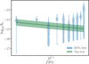 |
Fig. 2. Stochastic GW background predicted by our model (green) and the free spectrum measured by EPTA (blue). The 90% confidence intervals centred at the median for the amplitude of the GW background in the first and last bins, i.e., at frequencies 1/(10 yr) and 1/(1 yr), are |
In this work, we did not fit for the M* − MBH relation, but we perform a cross validation by comparing our results at z = 0 with the fit from Greene et al. (2020) (‘All’, including scatter), which is based on a large compilation of galaxies. At higher redshifts, we compare to the fits from Pacucci et al. (2023), derived from JWST data at redshifts z = 4 to 7.
4.2. Computation of the likelihood and sampling
Given the current uncertainty on the LF, we wished to explore a scenario where the true LF lies somewhere between the fits proposed in Shen et al. (2020) and Lacy et al. (2015). We denote ΦLacy(LBH, z0) and ΦShen(LBH, z0) the mean of the fits from Lacy et al. (2015) and Shen et al. (2020) respectively, and σLacy(LBH, z0) and σShen(LBH, z0) their standard deviations (in log space). For a given redshift, we defined a probability distribution pLF(log10Φ, LBH, z0) that, in each luminosity bin, is flat between min(log10ΦLacy − σLacy, log10ΦShen − σShen) and max(log10ΦLacy + σLacy, log10ΦShen + σShen) and beyond these limits falls as a Gaussian with standard deviation σLacy or σShen accordingly.
Our likelihood for the LF of a given set of parameters Λ, ℒLF(Λ, LBH, z0), was obtained by including the Poisson error on the LF computed from simulations so that
 (27)
(27)
where p(Φ|Λ) is a normal distribution with mean given by Eq. (11) and standard deviation Eq. (12). In practice, we performed a Monte Carlo integration, drawing samples for Φ from this normal distribution, truncating to positive values of Φ5. The total log-likelihood at z0 was obtained by summing over the luminosity bins in a z0-dependent range:
 (28)
(28)
Finally, the LF log-likelihood was obtained by summing over the different redshifts we wished to fit:
 (29)
(29)
Similarly, we used the EPTA posteriors (Antoniadis et al. 2023a,b,c, 2024a,b) on log10ρc, denoted by pPTA(log10ρc), to define the PTA likelihood in a given frequency bin f0 as
 (30)
(30)
We took p(log10(hc)|Λ) to be a normal distribution and the mean and error were computed from Eqs. (19)–(21)6. We performed a Monte Carlo integration using the samples of pPTA(log10ρc) taht were provided with the EPTA data release.
In this work, as a fiducial result, we fitted the LF at z = 0.25, 0.5, 3 and 6. For z0 = 0.25, we fited in the range of luminosities [1010, 1011.5] L⊙, for 0.5, in the range [1010, 1012] L⊙, while for z0 = 3 and 6, we fitted in the range [1012, 1014] L⊙ and [1011.5, 1013.5] L⊙ respectively.
Since we assumed MBH binaries to be on circular orbits, the slope of the GW background is constrained to −2/3, see Eq. (18). Fitting our model on the whole GW frequency range would therefore give the EPTA data a too large relative weight in the total fit without giving it the flexibility to better accommodate the GW spectrum as a whole. To facilitate comparison with previous works (Antoniadis et al. 2024a; Barausse et al. 2023) and because the way in which we estimate the PTA spectrum (assuming a normal distribution) is more accurate at low frequencies (Lamb & Taylor 2024), we focused on the frequency bin at f0 = 1/(10 yr).
Finally, we assigned zero likelihood to simulations that produce MBHs at z = 0 with masses exceeding 1012 M⊙, as these are unrealistically massive. In our model, such MBHs can form from heavy seeds, ∼106 M⊙, which later accrete in burst mode with Eddington ratios reaching up to 10. By z ∼ 7, these MBHs typically have masses around 108 − 109 M⊙, and since we limit accretion only at lower redshifts, there is no mechanism to prevent them from continuing to grow, potentially reaching masses incompatible with observations. A more physically motivated accretion model – based on the available mass reservoir, rather than on Eddington ratios and accretion times – would likely prevent the formation of these excessively large MBHs. However, since these are extreme outliers in our simulations (i.e., they appear in very few of the simulations that survive fitting to the LF and/or GW spectrum and in small numbers), we adopted this simple approach for now, leaving the implementation of a more refined accretion description for future work.
The priors used on the parameters of POMPOCO are detailed in Table 1. We explored the parameter space with an MCMC using the Eryn sampler (Karnesis et al. 2023). Since it is computationally cheap to run serially several sets of parameters for a given merger tree, we used many walkers (∼500) and ran the sampler only for a few steps (a few hundred).
5. Combined fit to the luminosity function and the gravitational-wave background
Our results for the LF, the GW background and the M* − MBH relation at z = 0 are shown in Figs. 1, 2 and 3 respectively. In each case, we present in green our model’s median (solid line) and 90% confidence interval (shaded region), as well as the observational data.
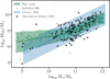 |
Fig. 3. Relation of the stellar mass and MBH mass at redshift z = 0. We compare our results, in green, with the fit of the local relation from Greene et al. (2020) (‘all’), in blue, and the data also compiled in Greene et al. (2020), in black. Green points show a (random) subsample of MBHs produced in our simulations. |
In Fig. 1, the light pink area denotes the region between the fits from Lacy et al. (2015) (pink) and Shen et al. (2020) (purple) where we allow the observational LF to reside. The recovered LF is remarkably consistent with observations at all redshifts – including those for which we do not explicitly fit. Note that our LF vanishes at high luminosities because of the finite number of DM haloes we simulate, which does not allow us to generate the rare MBHs behind the very bright end of the LF.
The GW spectrum (Fig. 2) we recover aligns well with the EPTA data (in blue) though our median lies slightly lower. This suggests our results might be better compatible with the reduced amplitude of Goncharov et al. (2024), obtained by adopting an observationally driven model for the pulsar noise. To facilitate comparison to Agazie et al. (2023b), we report the median of the GW background at two reference frequencies, together with the errors defining a 90% confidence region:
-
![Mathematical equation: $ h_c[1/(10\,\mathrm{yr})]=4.8^{+5.1}_{-2.7}\times 10^{-15} $](/articles/aa/full_html/2025/08/aa53027-24/aa53027-24-eq38.gif) ,
, -
![Mathematical equation: $ h_c[1/(1\,\mathrm{yr})]=1.0^{+1.1}_{-0.6}\times 10^{-15} $](/articles/aa/full_html/2025/08/aa53027-24/aa53027-24-eq39.gif) .
.
As a comparison, if, instead of performing the fiducial fit to the LF and PTA described in Sect. 4.2, we use POMPOCO to fit only for the LF of Shen et al. (2020) across redshifts, we obtain the following estimates:
-
![Mathematical equation: $ h_c[1/(10\,\mathrm{yr})]=3.9^{+7.0}_{-2.5}\times 10^{-16} $](/articles/aa/full_html/2025/08/aa53027-24/aa53027-24-eq40.gif) ,
, -
![Mathematical equation: $ h_c[1/(1\,\mathrm{yr})]=8.0^{+14.3}_{-5.1}\times 10^{-17} $](/articles/aa/full_html/2025/08/aa53027-24/aa53027-24-eq41.gif) .
.
The median values in the latter case are more than one order of magnitude below the ones reported above. Within the model itself, there is not so much the possibility of having a much lower LF at high z and producing a high GW background. In physical terms, a higher LF means higher density of BHs and so this is why the model can match the EPTA results. We recall that we assume MBH binaries to be circular, therefore the slope of the GW background spectrum is fixed to be −2/3 (see Eq. (18)). Including eccentricity and/or interactions with the environment would allow for a more flexible and shallower spectrum (Enoki & Nagashima 2007; Bonetti et al. 2018b; Antoniadis et al. 2024a; Ellis et al. 2024a). We plan to explore these possibilities in future work.
The resulting M* − MBH relation at z = 0 (Fig. 3) is in good agreement with the fit from Greene et al. (2020) (in blue), particularly in the region where most of the observational data (black points) are concentrated. A random sub-sample of individual MBHs from our simulations (green dots) shows that our model is capable of producing the most massive BHs observed in galaxies with M* ∼ 1011 M⊙, while also producing MBHs of 107 − 108.5 M⊙ in galaxies with M* ≥ 1011 M⊙. While these MBHs are clear outliers, our model is able to reproduce them, a feature that some other models find challenging, as discussed in Habouzit et al. (2021).
Our model predicts a break in the M* − MBH relation for galaxies with mass M* < 1010.5 M⊙. This originates from the break in the Mh − M* relation. The relation predicted directly by our model, Mh − MBH, does not show such a break at small MBH masses (see Fig. A.1 in the Appendix). This break is rather introduced by our use of the Mh − M* relation of Moster et al. (2010), which shows one precisely at Mh ∼ 1012 M⊙, corresponding to M* ∼ 1010.5 M⊙. Such a break is also observed in some cosmological simulations (Habouzit et al. 2021), and is imputed to the transition between SN feedback, suppressing MBH accretion in low-mass galaxies and AGN feedback, which leads to self-regulation of MBH accretion in high-mass galaxies and quenches star formation. For M* < 1010 M⊙, the median MBH mass is of order 107 M⊙ and lies above observations, with a shallower slope. We note, however, that there are only a few observations with M* < 1010 M⊙, so that the fit of Greene et al. (2020) is dominated by massive galaxies, and might not be accurate for low-mass galaxies. Ultimately, most observations in low-mass galaxies are within our 90% confidence region, and even those outside can actually be reproduced as outliers of our distribution (green points). In any case, we have checked that this potential overestimate of MBHs with mass 107 M⊙ does not impact our results on the PTA background, which is fully dominated by MBHs with mass > 108 M⊙.
At the massive galaxies end, our M* − MBH relation shows a break at M* ≳ 1012 M⊙ and slightly underestimates the mass of MBHs with respect to the observational fit. We note, however, that there is only one data point in this region (M* ≳ 1012 M⊙), so the fit might not be valid for these galaxies. As discussed in Appendix A, we have verified that this potential underestimation of the MBH masses should have a small impact on the stochastic GW background. In short, the reason is that this affects MBHs in more massive haloes, which are heavily suppressed by the Press-Schechter mass function, and therefore contribute little to the background.
We show the M* − MBH relation at higher redshift in Fig. 4. For z = 4, 5 and 6, we plot the AGN candidates from JWST observations in the redshift range z = 4 to 7 reported by Harikane et al. (2023), Übler et al. (2023), Maiolino et al. (2024), Li et al. (2025a). Since the Mh − M* relation from Moster et al. (2010) is calibrated for M* ≳ 108 M⊙, we restrict our plot to this stellar mass range. Additionally, the redshift evolution of their fit is only calibrated up to z ∼ 3.5, so our results at higher redshifts are based on extrapolation. In order to mimic selection effects in this dataset, we also show in dark green our relation when restricting to MBHs with LBH ≥ 1011 L⊙. Most data points are within the range predicted by our model when imposing this cut. Note that, when computing the M* − MBH relation predicted by POMPOCO, we also count MBHs in a binary as a single BH using the total mass of the binary, as described in Sect. 3.2, because it is usually challenging for observations to distinguish a single MBH from a binary at close separations, although some candidates have beed identified (Maiolino et al. 2024). We also show the fit to the local relation of Greene et al. (2020), and the fit of Pacucci et al. (2023), which is based on the same high redshift data points shown in Fig. 4 (except for the latest from Li et al. 2025a). We caution the reader that the underlying intrinsic M* − MBH relation at high redshift, once selection biases are accounted for, is still debated (Pacucci et al. 2023; Li et al. 2025b), as we do not know yet if a large population of undetected MBHs with lower mass ratio between MBH and M* exists.
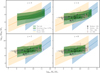 |
Fig. 4. Relation of the MBH mass and stellar mass at redshift z = 3, 4, 5, and 6. The darker green regions represent our results when restricting to MBHs with luminosity larger than 1011 L⊙, in order to mimic selection effects at high redshift. For z = 4, 5 and 6, we show JWST observations in the redshift range z = 4 to 7 (Maiolino et al. 2024; Übler et al. 2023; Harikane et al. 2023; Li et al. 2025a), some of which were used to obtain the fit of Pacucci et al. (2023) (light orange, excluding the more recent data of Li et al. 2025a). For comparison, we also show the fit to the observed local relation (light blue) of Greene et al. (2020). |
Overall, our model predicts a population in the same locus as the observations, although the slope is shallower than the fits of Greene et al. (2020) and Pacucci et al. (2023). Indeed, our model predicts a sizeable population of MBHs with mass almost comparable with the host galaxy mass in low-mass galaxies. We leave a deeper investigation of the possible causes for this discrepancy to future work. Conversely, the model does not include many very high-mass BHs (> 109 M⊙): this is related again to our simulated merger trees, which do not include the massive and rare haloes hosting the MBHs powering quasars at very bright end of the LF. At z = 3 and 4, we can see that our model starts to build up to the steeper local M* − MBH relation of Greene et al. (2020).
Overall, our analysis demonstrates that observations of the LF and of the (likely) GW background observed by PTAs can find a consistent description in our physical model, provided we allow for a more abundant population of AGN compared to global fits of the AGN LF based mainly on optical/UV/X-ray, pre-JWST data.
We show the posterior distribution of the parameters of our model in Figs. 5 and 6. For the sake of readability, the first figure shows the parameters controlling the seeding and merger delays, and the second figure those controlling accretion. We do not observe strong correlations between these two groups of parameters.
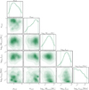 |
Fig. 5. Posterior on the model parameters related to seeding and BH mergers when fitting for the LF and GW background. We show the mean and standard deviation of the log-normal distribution of seed BH masses, μseed and σseed; the minimum mass of haloes seeded Mh, seed and the seeding probability fseed; the delay of binary BH mergers (in addition to halo dynamical friction), tdelay. |
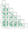 |
Fig. 6. Posterior on the model parameters related to accretion when fitting for the LF and the GW background. We show the slope of the power-law distribution γburst and the duration tburst of burst accretion; the mean and standard deviation of the log-normal distribution of steady accretion rates, μsteady and σsteady; the redshift zcut below which accretion is shut off for heavier MBHs; the slope of the increase of the shut-off mass, mcut, 0 at z = 0, with redshift, αcut. |
We obtain a relatively good constraint on the properties of haloes that are seeded, coming from the abundance of BHs in the Universe at different redshifts (i.e., the normalisation of the LF). Our model suggests that ∼10% of haloes with Mh ≳ 107 M⊙ at z ∼ 20 should host an MBH seed7. The range of values favoured for Mh, seed is more compatible with the prediction of relatively heavy seed models for the formation of seeds (see Regan & Volonteri 2024, for an overview and discussion). We obtain a broad posterior on the mean seed mass μseed, but with a clear preference for μseed ≳ 103 M⊙, in better agreement with the predictions of non-extreme heavy seed models (Volonteri et al. 2021). The tendency towards large values of σseed suggests that we tend to prefer broad initial distributions for the mass seed. This is likely due to the need to accommodate observations spanning a broad range of MBH masses, together with the restrictive shape of the seed mass distribution currently adopted in POMPOCO (a single Gaussian). Allowing for a combination of seeding channels (e.g. each having its own μseed and σseed) might improve this, but at the cost of increasing the parameter space. We expect that LISA will allow us to better identify the contribution of different seeding channels compared to current observations (Gair et al. 2011; Sesana et al. 2011; Klein et al. 2016; Toubiana et al. 2021).
We find large delays in MBH mergers to be strongly disfavoured, with tdelay ≲ 1 Gyr at 90% confidence. We recall this is an additional delay to the DF timescale following halo mergers and that we have considered a single value for all MBHs, without a mass or redshift dependence. Our findings are in line with those of Antoniadis et al. (2024a), Barausse et al. (2023), Agazie et al. (2023b), which found that PTA observations favour MBH binaries merging efficiently following galaxy mergers.
Moving on to the accretion parameters, the posterior on γburst suggests a log-flat distribution for fEdd in burst mode following major halo mergers, favouring the occurrence of super-Eddington accretion episodes. These burst episodes are estimated to last a few dozen million years, in agreement with the findings from Hopkins et al. (2006), Capelo et al. (2015). On average, burst accretion episodes increase the MBH mass by a factor of 1.2, rising to 2.8 in the case of super-Eddington episodes. The parameters of steady-mode accretion, in turn, are poorly constrained individually. The anti-correlation between μsteady and σsteady means, however, that ∼10% of the MBHs that accrete in this mode have fEdd > 10−2 and ∼4% have fEdd > 10−1. When we label these as AGN, this suggests that the AGN fraction is in the range 4 − 10% at ‘cosmic noon’, which in our model corresponds to z ∼ zcut. This is in good agreement with observations in different parts of the electromagnetic spectrum, which suggest an AGN fraction at z ∼ 1 − 3 in the range 1 − 10% (Aird et al. 2012; Trump et al. 2013; Donley et al. 2012). The strong correlations between γburst and tburst and between μsteady and σsteady point to the fact that a more physically driven approach to describe accretion, for instance based on a reservoir tracking the amount of mass available to accrete, might be possible, allowing to reduce the number of parameters in our model. We leave this exploration for future work.
Finally, our results do support the anti-hierarchical hypothesis for the growth of MBHs, as we observe a clear preference for accretion to shut off below zcut ∼ 2.5 with mcut, 0 ∼ 6 × 10⁶ M⊙. Although not very well constrained, the evolution parameter for the cut-off mass with redshift, αcut, does seem to favour strictly positive values, leading to the estimate that accretion is suppressed at zcut ∼ 2.5 for MBHs with mass ≳108 M⊙. The inferred value of zcut is in good agreement with observations and more complete numerical simulations, which estimate the peak of accretion to be in the range z = 2 − 3 (Merloni 2004; Hirschmann et al. 2012, 2014). Using our M* − MBH relation, we see that the preferred value of mcut, 0 corresponds to a stellar mass of ∼8 × 10¹⁰ M⊙, in good agreement with where the break in the Mh − M* relation of Moster et al. (2010) lies, for Mh ∼ 1012 M⊙. This break has been interpreted as being due to the combined effect of the feedback from supernovae (in smaller haloes) and AGNs (in larger haloes) (Croton et al. 2006; Shankar et al. 2006; Bower et al. 2006; Somerville et al. 2008).
The fact that the inferred values of the parameters entering POMPOCO are overall in good agreement with findings from observations and/or more complete numerical simulations reinforces our confidence that our model is able to capture the key features driving the formation and evolution of MBHs and that our conclusions on the compatibility of the LF and the GW background are robust.
6. Merger rates and LISA predictions
Next, we turn to the predictions for merger rates and LISA observations based on our fits to the LF and the GW stochastic background. We compute the yearly rate as a function of MBH binary parameters, as well as the total rate (per year), following the procedure described in Sect. 3.4. To estimate the LISA detection rate, we restrict to events with signal-to-noise ratio (S/N) above 10, which we assume to be the threshold for detection in a 4-year mission. The S/N of the sources is computed assuming the “Proposal” noise curve (Amaro-Seoane et al. 2017) and using the IMRPhenomXHM model (García-Quirós et al. 2020) for the waveform. Since we do not track the evolution of spins in our simulations, for simplicity, we attribute a spin 0 to both BHs in a binary when computing S/Ns. We do not expect our results for the expected number of detections to be much affected by this choice, since spins, at the level of the whole population, introduce a second order correction to the detectability of the sources. For each event, we draw the sky location, the phase at coalescence, the polarisation and the inclination angle isotropically.
Figure 7 shows the posterior distribution of the merger rate per year, while Figs. 8 and 9 present this rate as a function of the total binary mass, mt, and redshift, z, respectively. The thick lines represent the median values, with the shaded regions indicating the 90% confidence intervals, and the thin lines illustrating individual realisations of our model. Green curves show the intrinsic rate, while the light green ones show the rate of events detectable with LISA. Our predictions for LISA cover a wide range, with the expected number of merger events varying from a few to thousands per year.
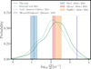 |
Fig. 7. Prediction of the yearly rate of MBH mergers after fitting for the LF and the GW background measured by EPTA. The solid curve shows the intrinsic rate, the dotted one the rate of detetable events, assuming an S/N threshold of 10. For comparison, we also report the predictions for the intrinsic rate of other models from the literature (see text for description). For Q3-nod, Q3-d and PopIII-d, the shaded areas show the range reported in reference Barausse et al. (2023) (the lower bound corresponding to finite resolution results, and the upper bound to results extrapolated to infinite resolution). For model HS-nod-SN-high-accr, we only report finite resolution results (i.e. a lower bound) as the extrapolation was not provided in reference Barausse et al. (2023). |
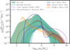 |
Fig. 8. Prediction of the yearly rate of mergers as a function of the total source-frame mass of the binary. Thick lines show the median and shaded areas the 90% confidence region after fitting for the LF and the GW background of EPTA. The green curves correspond to the intrinsic merger rate, while the light green curves show the rate of events detectable by LISA, assuming an S/N threshold of 10. Predictions from other models are included for comparison. |
In Figs. 7, 8 and 9 we also compare our results for the intrinsic rate with those of other models from the literature, selecting ones that have shown good agreement with EPTA (Antoniadis et al. 2024a): models Q3-nod, Q3-d and PopIII-d from Klein et al. (2016), model HS-nod-SN-high-accr from Barausse et al. (2023), and model Loud from Izquierdo-Villalba et al. (2024). We refer to the upcoming paper by members of the LISA astrophysics working group for a more exhaustive comparison of LISA predictions in different SAMs and cosmological simulations (LISA Astrophysics Working Group, in prep.).
The models Q3-nod, Q3-d and HS-nod-SN-high-accr assume that MBHs form from heavy seeds (from the collapse of protogalactic discs Volonteri et al. 2008), while PopIII-d assumes that they form from the remnant of Pop III stars (Madau & Rees 2001). Models HS-nod-SN-high-accr and Q3-nod also feature no delays between galaxy mergers and MBH mergers (although they include delays between halo and galaxy mergers), while PopIII-d and Q3-d do include delays due to stellar hardening, gas-driven migration and triple black-hole interactions that affect MBH binaries. Moreover, in model HS-nod-SN-high-accr the influx of gas into the nuclear regions hosting MBHs is boosted by a factor ∼4, to achieve better agreement with the PTA results (Antoniadis et al. 2024a; Barausse et al. 2023).
The Loud model by Izquierdo-Villalba et al. (2024) uses the L-Galaxies SAM with a mix of heavy and light seeds to track MBH binary evolution after galaxy mergers. It considers three phases: dynamical friction, hardening, and GW emission. The dynamical friction phase of the satellite MBHs lasts for a time given by Binney & Tremaine (2008) and starts at the radius at which the tidal forces stripped 80% of the galaxy stellar mass. At the end of this phase, the MBHs form a gravitational bound binary, entering the hardening and GW inspiral phases whose separation and eccentricity are evolved consistently based on whether the environment is gas-rich or gas-poor. The model also accounts for triple interactions and, during the MBH binary growth, an anticorrelation between the accretion rate of the primary and secondary MBH (preferential accretion). Specifically, in the Loud model, the efficiency of MBH accretion is boosted to reproduce the GW background measured by EPTA.
Our predictions agree best with the “Q3-nod” model, which assumes that MBHs form from heavy seeds and merge soon after galaxy mergers, which aligns well with the preferred values of μseeds and tdelay in our analysis. The HS-nod-SN-high-accr model, which makes similar hypotheses for the seeding and the delay, also shows good agreement with our results, the main difference being its large merger rate at high redshift8. As values of μseed ∼ 102 M⊙ are also allowed by our analyis, the PopIII-d model is also mostly compatible with our results, although it is not preferred. This confirms that LISA will play a crucial role in disentangling formation scenarios.
The Loud model predicts mergers only from z ≲ 10, in tension with our results. This discrepancy may stem from the assumption in POMPOCO that the delay between galaxy and MBH mergers is independent of galaxy mass. In our model, this additional delay beyond the DF timescale is parametrised by tdelay is applied uniformly to all mergers. MBH binaries resulting from low-mass galaxy mergers are expected to experience longer formation and coalescence timescales than those in more massive systems, however. Supporting this hypothesis, the Q3-d model, which includes a post-galaxy-merger delay, yields a redshift distribution similar to the Loud model, whereas the Q3-nod model, which omits this delay, aligns more closely with our predictions. We plan to refine this aspect in future work. Note that this would not necessarily lead to a reduction in the PTA GW background, since delays following mergers of more massive galaxies–those hosting the MBHs that dominate the background could be relatively short. In this sense, our tdelay parameter may be more reflective of the delay timescales in such massive systems. In terms of total mass, the predictions of the Loud model are generally consistent with our results across most of the mass spectrum, with the exception of the high-mass end. There, it predicts significantly more mergers involving MBH binaries with mt ∼ 109 M⊙, as a result of enhanced accretion in the model, which was introduced to fit the GW background spectrum. This is compensated in our model by a larger number of mergers occurring at low redshift, allowing us to obtain a good match with the EPTA measurement.
Regarding LISA detections, our best estimate of a few hundred events per year (see Fig. 7) is most consistent with the predictions of the Q3-nod model (∼100–200 yr−1) and the PopIII-d model (∼50–100 yr−1). In contrast, the predicted detection rates of ∼10 yr−1 (Loud) and 10–20 yr−1 (Q3-d) fall in the lower tail of our distribution, while the HS-nod-SN-high-accr model, with its prediction of ∼2000 yr−1, lies in the upper tail. Detection rates are taken from Table 1 of Barausse et al. (2023) for the Q3-nod, Q3-d, PopIII-d, and HS-nod-SN-high-accr models, and from Table 1 of Izquierdo-Villalba et al. (2024) for the “Loud” model.
This comparison demonstrates that, even in its current version, POMPOCO is flexible enough to describe a range of MBH populations – a key goal of the model. To fully exploit the potential of LISA to distinguish between different formation mechanisms, however, it will be necessary to explicitly include more than one formation channel in our model in the near future.
7. Discussion and conclusions
The number of observational probes into the population of MBHs in the Universe has recently increased rapidly, and even more probes are expected in the near future. Preliminary results from the JWST already reveal intriguing discrepancies with previously accepted models, and it is anticipated that the upcoming observations will provide deeper insights. Additionally, PTA collaborations are on the verge of confirming the detection of the GW background in the nanohertz frequency band, generated by inspiralling MBH binaries. In the next decade, the launch of LISA will revolutionise our understanding of MBH formation and evolution by detecting a so far unobserved population of merging MBHs. To fully capitalise on these upcoming observations, it is essential to develop a framework that can comprehensively compare theoretical predictions with a wide variety of observational data.
To do this, we have developed the model POMPOCO, which stands for Parametrisation Of the Massive black hole POpulation for Comparison to Observations. It features 12 free parameters that are designed to effectively describe the formation and evolution of MBHs within DM halo merger trees. The computational efficiency of POMPOCO, compared to full cosmological simulations and SAMs allows us to explore a wide range of parameter space and to identify the configurations that fit the selected datasets best.
In this study, we used POMPOCO to demonstrate the consistency between the LF and the amplitude of the PTA GW background, in particular, for an enhanced LF at high redshift, as suggested by extrapolating the results from Lacy et al. (2015) and by the preliminary findings from the JWST (Harikane et al. 2023; Maiolino et al. 2024; Greene et al. 2024; Matthee et al. 2024; Taylor et al. 2025; see also Somalwar & Ravi 2025; Ellis et al. 2024b; Padmanabhan & Loeb 2024 for a similar analysis. The authors found a consistency between PTA observations and JWST black hole candidates). To achieve this, we defined a likelihood function that accommodated the LF at different redshifts between the comprehensive fits from Shen et al. (2020) and the fits to mid-IR observations from Lacy et al. (2015), and alongside the amplitude of the GW background inferred for the first frequency bin of the EPTA data. We then conducted a full Bayesian analysis. While our inferred GW spectrum clearly agrees with the EPTA data, the median of our prediction lies slightly below EPTA’s one, which might indicate a lower background, as proposed by Goncharov et al. (2024). Although we focused on the case of circular binaries in this work, we hope to include the effect of eccentricity when fitting to PTA data in future studies.
We verified our results against the observed M* − MBH relation at z = 0, for which we did not explicitly fit. The results agree very well with the fit by Greene et al. (2020). Furthermore, our model is capable of reproducing even some of the MBHs that were observed outside of the main distribution. Many models struggle with this feature (Habouzit et al. 2021).
A key strength of POMPOCO lies in its ability to provide a posterior distribution for the model parameters when simultaneously fitting to the LF and the GW background. For instance, our Bayesian analysis showed that approximately 10% of haloes with a mass ≳107 M⊙ at z ∼ 20 should host an MBH seed, with characteristic masses ranging from 103 and 5 × 10⁶ M⊙. Additionally, we estimated that a fraction of MBHs undergoes super-Eddington accretion in burst episodes lasting a few dozen million years. At cosmic noon, we predict an AGN fraction of 4 − 10% and that the peak of accretion occurs at z ∼ 2.5. Finally, we found that MBHs with masses ≳108 M⊙ experience accretion suppression by z ∼ 2.5 and that this suppression extends to MBHs with masses ≳6 × 10⁶ M⊙ by z = 0. These estimates are consistent with the findings of more detailed numerical simulations and observations. This suggests that POMPOCO captures the essential features that drive the MBH formation and evolution.
Our model predictions for LISA are broad, but agree better with some scenarios than with others. In particular, they are more consistent with SAMs that assume that MBHs originate from heavy seeds and merge efficiently following galaxy mergers, such as the Q3-nod model (Klein et al. 2016) and HS-nod-SN-high-accr (Barausse et al. 2020). Discrepancies with the Q3-d (Klein et al. 2016) and Loud Izquierdo-Villalba et al. (2024) models in the distribution of merger redshifts suggest the need of introducing a dependence of the post-galaxy-merger delay on the mass of the host galaxy. Overall, POMPOCO is flexible enough to describe a variety of scenarios for merging MBHs while remaining compatible with current observations. To fully leverage the potential of LISA to distinguish between different formation scenarios, however, we plan to increase the flexibility of the seed distribution in our model.
Looking ahead, we aim to introduce several improvements to POMPOCO. In addition to incorporating eccentricity and other formation channels, we plan to model the spin evolution of MBHs, which is critically sensitive to the environment of merging MBH binaries (Berti & Volonteri 2008; Sesana et al. 2014; Spadaro et al. 2025). The inclusion of eccentricity and spins will also allow us to correctly model the impact of kicks following MBH mergers, which we neglected in this work, and which could lower the LISA rates. In this work, we fixed the radiative efficiency to 0.1, whereas it is expected to depend on the accretion rate and on the spin of the BHs (e.g. Merloni & Heinz 2008; Madau et al. 2014). When spins and the suppression of the radiative efficiency at very low and very high Eddington ratios are included in our model, it will properly account for this. Moreover, we intend to adopt a more physically motivated accretion model, such as one based on the mass reservoir available for accretion. This might reduce the parameter space and prevent the formation of unrealistically large MBHs. Finally, we also plan to incorporate a dependence of the time delay between galaxy mergers and the formation of MBH binaries on the masses of the host galaxies. It will be crucial to address these issues for fully extracting the astrophysical information encoded in the LISA observations and realising the immense potential of the observatory (Gair et al. 2011; Klein et al. 2016; Bonetti et al. 2019; Toubiana et al. 2021; Fang & Yang 2023; Langen et al. 2025; Spadaro et al. 2025).
Leaf haloes can be at z < zmax, if their mass drops below the mass resolution.
We exclude stellar mass seeds below m < 100 M⊙, as Smith et al. (2018), Shi et al. (2024) found that less than 1% can grow to contribute to the MBH population.
This numerical prefactor is related to the orbital parameters of the haloes. The value adopted in Volonteri et al. (2003) was motivated by numerical investigations.
For instance, if the posterior of zcut was to favour values close to 0, or the one of mcut, 0 values above the mass of most astrophysical BHs, for example 1011 M⊙, this would be a sign that the model does not need anti-hierarchical growth to fit the data.
Notice that we took the distribution on Φ to be normal, not on log10Φ, since it is Φ that is a weighted sum of Poisson processes. Converting the error on Φ into an error on log10Φ through the standard propagation of errors is justified only when the error is much smaller than the quantity, which is not necessarily the case in the high luminosity bins where we have few counts, and would lead to underestimating the impact of Poisson errors. Ideally, we should use the formalism of Bohm & Zech (2014) rather than assuming a normal distribution when the total count is small and Poisson errors are large.
In this case, we assumed a normal distribution on log10ρc because the errors on ρc2 is small enough so that propagation of error into log10ρc can be used.
These values should be interpreted with caution, in particular for fseed, due to the finite resolution of our DM halo merger trees. The minimum mass we resolve at z = 20 is ∼2 × 10⁶(Mh, 0/1014) M⊙. For the most massive haloes with a mass of 1015 M⊙ at z = 0, the minimum resolved mass therefore is above our best estimate for Mh, seed. Because we allowed all leaves above z = 10 to be seeded, however, haloes that fell below the mass resolution before z = 20 might still be seeded. Moreover, such heavy haloes are strongly suppressed by the Press-Schechter mass function and contribute little to our Universe. Therefore, we expect our estimates to be qualitatively meaningful, in particular for Mh, seed.
The larger merger rate at high redshift in model HS-nod-SN-high-accr is due to both the different threshold Toomre parameter used for seed formation in unstable protogalactic discs, and to better tracking of sub-resolution haloes hosting an MBH seed, see Barausse et al. (2023) for more details.
Acknowledgments
We are thankful to S. Grunewald for his precious help in making POMPOCO fit to run on the Hypatia cluster, to L. Speri for providing us the EPTA data, and to M. Habouzit for fruitful discussion. A.T. is supported by ERC Starting Grant No. 945155–GWmining, Cariplo Foundation Grant No. 2021-0555, MUR PRIN Grant No. 2022-Z9X4XS, MUR Grant “Progetto Dipartimenti di Eccellenza 2023-2027” (BiCoQ), and the ICSC National Research Centre funded by NextGenerationEU. L.S. acknowledges support from the UKRI guarantee funding (project no. EP/Y023706/1). M.V. and S.B. acknowledge funding from the French National Research Agency (grant ANR-21-CE31-0026, project MBH_waves). This work has received funding from the Centre National d’Etudes Spatiales. E.B. acknowledges support from the European Union’s H2020 ERC Consolidator Grant “GRavity from Astrophysical to Microscopic Scales” (Grant No. GRAMS-815673), the European Union’s Horizon ERC Synergy Grant “Making Sense of the Unexpected in the Gravitational-Wave Sky” (Grant No. GWSky-101167314), the PRIN 2022 grant “GUVIRP – Gravity tests in the UltraViolet and InfraRed with Pulsar timing”, and the EU Horizon 2020 Research and Innovation Programme under the Marie Sklodowska-Curie Grant Agreement No. 101007855. This work has been supported by the Agenzia Spaziale Italiana (ASI), Project n. 2024-36-HH.0, “Attività per la fase B2/C della missione LISA”.
References
- Agazie, G., Anumarlapudi, A., Archibald, A. M., et al. 2023a, ApJ, 951, L8 [NASA ADS] [CrossRef] [Google Scholar]
- Agazie, G., Anumarlapudi, A., Archibald, A. M., et al. 2023b, ApJ, 952, L37 [NASA ADS] [CrossRef] [Google Scholar]
- Agazie, G., Antoniadis, J., Anumarlapudi, A., et al. 2024, ApJ, 966, 105 [NASA ADS] [CrossRef] [Google Scholar]
- Aird, J., Coil, A. L., Moustakas, J., et al. 2012, ApJ, 746, 90 [CrossRef] [Google Scholar]
- Aird, J., Coil, A. L., & Georgakakis, A. 2018, MNRAS, 474, 1225 [NASA ADS] [CrossRef] [Google Scholar]
- Akins, H. B., Casey, C. M., Lambrides, E., et al. 2024, ArXiv e-prints [arXiv:2406.10341] [Google Scholar]
- Allevato, V., Shankar, F., Marsden, C., et al. 2021, ApJ, 916, 34 [NASA ADS] [CrossRef] [Google Scholar]
- Amaro-Seoane, P., Audley, H., Babak, S., et al. 2017, ArXiv e-prints [arXiv:1702.00786] [Google Scholar]
- Antoniadis, J., Arumugam, P., Arumugam, S., et al. 2023a, A&A, 678, A50 [CrossRef] [EDP Sciences] [Google Scholar]
- Antoniadis, J., Babak, S., Bak Nielsen, A. S., et al. 2023b, A&A, 678, A48 [Google Scholar]
- Antoniadis, J., Arumugam, P., Arumugam, S., et al. 2023c, A&A, 678, A49 [Google Scholar]
- Antoniadis, J., Arumugam, P., Arumugam, S., et al. 2024a, A&A, 685, A94 [NASA ADS] [CrossRef] [EDP Sciences] [Google Scholar]
- Antoniadis, J., Arumugam, P., Arumugam, S., et al. 2024b, A&A, 690, A118 [NASA ADS] [CrossRef] [EDP Sciences] [Google Scholar]
- Baldassare, V. F., Geha, M., & Greene, J. 2020, ApJ, 896, 10 [NASA ADS] [CrossRef] [Google Scholar]
- Barausse, E. 2012, MNRAS, 423, 2533 [NASA ADS] [CrossRef] [Google Scholar]
- Barausse, E., Dvorkin, I., Tremmel, M., Volonteri, M., & Bonetti, M. 2020, ApJ, 904, 16 [NASA ADS] [CrossRef] [Google Scholar]
- Barausse, E., Dey, K., Crisostomi, M., et al. 2023, Phys. Rev. D, 108, 103034 [NASA ADS] [CrossRef] [Google Scholar]
- Benson, A. J. 2012, New Astron., 17, 175 [NASA ADS] [CrossRef] [Google Scholar]
- Benson, A. J. 2017, MNRAS, 467, 3454 [NASA ADS] [CrossRef] [Google Scholar]
- Berti, E., & Volonteri, M. 2008, ApJ, 684, 822 [NASA ADS] [CrossRef] [Google Scholar]
- Bhowmick, A. K., Blecha, L., Torrey, P., et al. 2024, MNRAS, 531, 4311 [NASA ADS] [CrossRef] [Google Scholar]
- Binney, J., & Tremaine, S. 1987, Galactic Dynamics (Princeton: Princeton University Press) [Google Scholar]
- Binney, J., & Tremaine, S. 2008, Galactic Dynamics: Second Edition (Princeton: Princeton University Press) [Google Scholar]
- Boettner, C., Trebitsch, M., & Dayal, P. 2025, A&A, 693, A295 [NASA ADS] [CrossRef] [EDP Sciences] [Google Scholar]
- Bohm, G., & Zech, G. 2014, Nucl. Instrum. Meth. A, 748, 1 [Google Scholar]
- Bond, J. R., Cole, S., Efstathiou, G., & Kaiser, N. 1991, ApJ, 379, 440 [NASA ADS] [CrossRef] [Google Scholar]
- Bonetti, M., Haardt, F., Sesana, A., & Barausse, E. 2018a, MNRAS, 477, 3910 [Google Scholar]
- Bonetti, M., Sesana, A., Barausse, E., & Haardt, F. 2018b, MNRAS, 477, 2599 [NASA ADS] [CrossRef] [Google Scholar]
- Bonetti, M., Sesana, A., Haardt, F., Barausse, E., & Colpi, M. 2019, MNRAS, 486, 4044 [NASA ADS] [CrossRef] [Google Scholar]
- Bower, R. G. 1991, MNRAS, 248, 332 [NASA ADS] [CrossRef] [Google Scholar]
- Bower, R. G., Benson, A. J., Malbon, R., et al. 2006, MNRAS, 370, 645 [Google Scholar]
- Capelo, P. R., Volonteri, M., Dotti, M., et al. 2015, MNRAS, 447, 2123 [NASA ADS] [CrossRef] [Google Scholar]
- Cole, S., Lacey, C. G., Baugh, C. M., & Frenk, C. S. 2002, MNRAS, 319, 168 [NASA ADS] [CrossRef] [Google Scholar]
- Colpi, M. 2014, Space Sci. Rev., 183, 189 [Google Scholar]
- Colpi, M., Danzmann, K., Hewitson, M., et al. 2024, ArXiv e-prints [arXiv:2402.07571] [Google Scholar]
- Conroy, C., & White, M. 2012, ApJ, 762, 70 [Google Scholar]
- Croton, D. J., Springel, V., White, S. D. M., et al. 2006, MNRAS, 365, 11 [Google Scholar]
- Dayal, P., Rossi, E. M., Shiralilou, B., et al. 2019, MNRAS, 486, 2336 [Google Scholar]
- Donley, J. L., Koekemoer, A. M., Brusa, M., et al. 2012, ApJ, 748, 142 [Google Scholar]
- Dubois, Y., Volonteri, M., & Silk, J. 2014a, MNRAS, 440, 1590 [Google Scholar]
- Dubois, Y., Pichon, C., Welker, C., et al. 2014b, MNRAS, 444, 1453 [Google Scholar]
- Ellis, J., Fairbairn, M., Hütsi, G., et al. 2024a, Phys. Rev. D, 109, L021302 [NASA ADS] [CrossRef] [Google Scholar]
- Ellis, J., Fairbairn, M., Hütsi, G., et al. 2024b, A&A, 691, A270 [NASA ADS] [CrossRef] [EDP Sciences] [Google Scholar]
- Enoki, M., & Nagashima, M. 2007, Prog. Theor. Phys., 117, 241 [CrossRef] [Google Scholar]
- Fabian, A. C. 2012, ARA&A, 50, 455 [Google Scholar]
- Fang, Y., & Yang, H. 2023, MNRAS, 523, 5120 [NASA ADS] [CrossRef] [Google Scholar]
- Ferrarese, L., & Merritt, D. 2000, ApJ, 539, L9 [Google Scholar]
- Gair, J. R., Sesana, A., Berti, E., & Volonteri, M. 2011, Class. Quant. Grav., 28, 094018 [Google Scholar]
- García-Quirós, C., Colleoni, M., Husa, S., et al. 2020, Phys. Rev. D, 102, 064002 [CrossRef] [Google Scholar]
- Gardner, J. P., Mather, J. C., Clampin, M., et al. 2006, Space Sci. Rev., 123, 485 [Google Scholar]
- Gehren, T., Fried, J., Wehinger, P. A., & Wyckoff, S. 1984, ApJ, 278, 11 [NASA ADS] [CrossRef] [Google Scholar]
- Gilli, R., Norman, C., Calura, F., et al. 2022, A&A, 666, A17 [NASA ADS] [CrossRef] [EDP Sciences] [Google Scholar]
- Goncharov, B., Sardana, S., Sesana, A., et al. 2024, ArXiv e-prints [arXiv:2409.03627] [Google Scholar]
- Greene, J. E., Strader, J., & Ho, L. C. 2020, ARA&A, 58, 257 [Google Scholar]
- Greene, J. E., Labbe, I., Goulding, A. D., et al. 2024, ApJ, 964, 39 [CrossRef] [Google Scholar]
- Habouzit, M. 2024, ArXiv e-prints [arXiv:2405.05319] [Google Scholar]
- Habouzit, M., Li, Y., Somerville, R. S., et al. 2021, MNRAS, 503, 1940 [NASA ADS] [CrossRef] [Google Scholar]
- Harikane, Y., Zhang, Y., Nakajima, K., et al. 2023, ApJ, 959, 39 [NASA ADS] [CrossRef] [Google Scholar]
- Hartwig, T. 2019, Formation of the First Black Holes (World Scientific), 161 [Google Scholar]
- Hirschmann, M., Somerville, R. S., Naab, T., & Burkert, A. 2012, MNRAS, 426, 237 [NASA ADS] [CrossRef] [Google Scholar]
- Hirschmann, M., Dolag, K., Saro, A., et al. 2014, MNRAS, 442, 2304 [Google Scholar]
- Hopkins, P. F., Hernquist, L., Cox, T. J., et al. 2006, ApJS, 163, 1 [Google Scholar]
- Hopkins, P. F., Richards, G. T., & Hernquist, L. 2007, ApJ, 654, 731 [Google Scholar]
- Izquierdo-Villalba, D., Bonoli, S., Dotti, M., et al. 2020, MNRAS, 495, 4681 [NASA ADS] [CrossRef] [Google Scholar]
- Izquierdo-Villalba, D., Sesana, A., Colpi, M., et al. 2024, A&A, 686, A183 [NASA ADS] [CrossRef] [EDP Sciences] [Google Scholar]
- Kannan, R., Garaldi, E., Smith, A., et al. 2021, MNRAS, 511, 4005 [Google Scholar]
- Karnesis, N., Katz, M. L., Korsakova, N., Gair, J. R., & Stergioulas, N. 2023, MNRAS, 526, 4814 [Google Scholar]
- Klein, A., Barausse, E., Sesana, A., et al. 2016, Phys. Rev. D, 93, 024003 [NASA ADS] [CrossRef] [Google Scholar]
- Kocevski, D. D., Barro, G., McGrath, E. J., et al. 2023, ApJ, 946, L14 [NASA ADS] [CrossRef] [Google Scholar]
- Kokorev, V., Fujimoto, S., Labbe, I., et al. 2023, ApJ, 957, L7 [NASA ADS] [CrossRef] [Google Scholar]
- Kormendy, J., & Ho, L. C. 2013, ARA&A, 51, 511 [Google Scholar]
- Kormendy, J., & Richstone, D. 1995, ARA&A, 33, 581 [Google Scholar]
- Kulier, A., Ostriker, J. P., Natarajan, P., Lackner, C. N., & Cen, R. 2015, ApJ, 799, 178 [NASA ADS] [CrossRef] [Google Scholar]
- Lacey, C. G., & Cole, S. 1993, MNRAS, 262, 627 [NASA ADS] [CrossRef] [Google Scholar]
- Lacy, M., Ridgway, S. E., Sajina, A., et al. 2015, ApJ, 802, 102 [NASA ADS] [CrossRef] [Google Scholar]
- Lamb, W. G., & Taylor, S. R. 2024, ApJ, 971, L10 [NASA ADS] [CrossRef] [Google Scholar]
- Langen, V., Tamanini, N., Marsat, S., & Bortolas, E. 2025, MNRAS, 536, 3366 [Google Scholar]
- Latif, M. A., & Ferrara, A. 2016, PASA, 33, e051 [NASA ADS] [CrossRef] [Google Scholar]
- Li, J., Shen, Y., & Zhuang, M. Y. 2025a, ArXiv e-prints [arXiv:2502.05048] [Google Scholar]
- Li, J., Silverman, J. D., Shen, Y., et al. 2025b, ApJ, 981, 19 [Google Scholar]
- Lyu, J., Alberts, S., Rieke, G. H., et al. 2024, ApJ, 966, 229 [NASA ADS] [CrossRef] [Google Scholar]
- Madau, P., & Rees, M. J. 2001, ApJ, 551, L27 [Google Scholar]
- Madau, P., Haardt, F., & Dotti, M. 2014, ApJ, 784, L38 [NASA ADS] [CrossRef] [Google Scholar]
- Maiolino, R., Scholtz, J., Curtis-Lake, E., et al. 2024, A&A, 691, A145 [NASA ADS] [CrossRef] [EDP Sciences] [Google Scholar]
- Matthee, J., Naidu, R. P., Brammer, G., et al. 2024, ApJ, 963, 129 [NASA ADS] [CrossRef] [Google Scholar]
- McConnell, N. J., & Ma, C.-P. 2013, ApJ, 764, 184 [Google Scholar]
- Merloni, A. 2004, MNRAS, 353, 1035 [NASA ADS] [CrossRef] [Google Scholar]
- Merloni, A., & Heinz, S. 2008, MNRAS, 388, 1011 [NASA ADS] [Google Scholar]
- Monaco, P., Fontanot, F., & Taffoni, G. 2007, MNRAS, 375, 1189 [NASA ADS] [CrossRef] [Google Scholar]
- Moster, B. P., Somerville, R. S., Maulbetsch, C., et al. 2010, ApJ, 710, 903 [Google Scholar]
- Ni, Y., Di Matteo, T., Bird, S., et al. 2022, MNRAS, 513, 670 [NASA ADS] [CrossRef] [Google Scholar]
- Oesch, P. A., Brammer, G., Naidu, R. P., et al. 2023, MNRAS, 525, 2864 [NASA ADS] [CrossRef] [Google Scholar]
- Onoue, M., Inayoshi, K., Ding, X., et al. 2023, ApJ, 942, L17 [NASA ADS] [CrossRef] [Google Scholar]
- Pacucci, F., Nguyen, B., Carniani, S., Maiolino, R., & Fan, X. 2023, ApJ, 957, L3 [CrossRef] [Google Scholar]
- Padmanabhan, H., & Loeb, A. 2024, A&A, 684, L15 [NASA ADS] [CrossRef] [EDP Sciences] [Google Scholar]
- Parkinson, H., Cole, S., & Helly, J. 2008, MNRAS, 383, 557 [Google Scholar]
- Pérez-González, P. G., Barro, G., Rieke, G. H., et al. 2024, ApJ, 968, 4 [CrossRef] [Google Scholar]
- Phinney, E. S. 2001, ArXiv e-prints [arXiv:astro-ph/0108028] [Google Scholar]
- Press, W. H., & Schechter, P. 1974, ApJ, 187, 425 [Google Scholar]
- Reardon, D. J., Zic, A., Shannon, R. M., et al. 2023, ApJ, 951, L6 [NASA ADS] [CrossRef] [Google Scholar]
- Rees, M. J. 1988, Nature, 333, 523 [Google Scholar]
- Regan, J., & Volonteri, M. 2024, Open J. Astrophys., 7, 72 [NASA ADS] [CrossRef] [Google Scholar]
- Reines, A. E., Sivakoff, G. R., Johnson, K. E., & Brogan, C. L. 2011, Nature, 470, 66 [Google Scholar]
- Reines, A. E., Greene, J. E., & Geha, M. 2013, ApJ, 775, 116 [Google Scholar]
- Ricarte, A., & Natarajan, P. 2018, MNRAS, 474, 1995 [Google Scholar]
- Ricarte, A., Tremmel, M., Natarajan, P., & Quinn, T. 2019, MNRAS, 489, 802 [NASA ADS] [CrossRef] [Google Scholar]
- Sahu, N., Graham, A. W., & Davis, B. L. 2019, ApJ, 876, 155 [NASA ADS] [CrossRef] [Google Scholar]
- Scholtz, J., Maiolino, R., D’Eugenio, F., et al. 2025, A&A, 697, A175 [NASA ADS] [CrossRef] [EDP Sciences] [Google Scholar]
- Schramm, M., & Silverman, J. D. 2013, ApJ, 767, 13 [NASA ADS] [CrossRef] [Google Scholar]
- Scott, N., Graham, A. W., & Schombert, J. 2013, ApJ, 768, 76 [NASA ADS] [CrossRef] [Google Scholar]
- Sesana, A., Vecchio, A., & Colacino, C. N. 2008, MNRAS, 390, 192 [NASA ADS] [CrossRef] [Google Scholar]
- Sesana, A., Gair, J., Berti, E., & Volonteri, M. 2011, Phys. Rev. D, 83, 044036 [NASA ADS] [CrossRef] [Google Scholar]
- Sesana, A., Barausse, E., Dotti, M., & Rossi, E. M. 2014, ApJ, 794, 104 [NASA ADS] [CrossRef] [Google Scholar]
- Shankar, F. 2013, Class. Quant. Grav., 30, 244001 [Google Scholar]
- Shankar, F., Lapi, A., Salucci, P., De Zotti, G., & Danese, L. 2006, ApJ, 643, 14 [NASA ADS] [CrossRef] [Google Scholar]
- Shankar, F., Allevato, V., Bernardi, M., et al. 2020, Nat. Astron., 4, 282 [Google Scholar]
- Shen, X., Hopkins, P. F., Faucher-Giguère, C.-A., et al. 2020, MNRAS, 495, 3252 [Google Scholar]
- Shi, Y., Kremer, K., & Hopkins, P. F. 2024, A&A, 691, A24 [NASA ADS] [CrossRef] [EDP Sciences] [Google Scholar]
- Small, T. A., & Blandford, R. D. 1992, MNRAS, 259, 725 [NASA ADS] [Google Scholar]
- Smith, B. D., Regan, J. A., Downes, T. P., et al. 2018, MNRAS, 480, 3762 [NASA ADS] [CrossRef] [Google Scholar]
- Soltan, A. 1982, MNRAS, 200, 115 [Google Scholar]
- Somalwar, J. J., & Ravi, V. 2025, ApJ, 982, 195 [Google Scholar]
- Somerville, R. S., Hopkins, P. F., Cox, T. J., Robertson, B. E., & Hernquist, L. 2008, MNRAS, 391, 481 [NASA ADS] [CrossRef] [Google Scholar]
- Spadaro, A., Buscicchio, R., Izquierdo-Villalba, D., et al. 2025, Phys. Rev. D, 111, 023004 [Google Scholar]
- Springel, V., Pakmor, R., Pillepich, A., et al. 2017, MNRAS, 475, 676 [Google Scholar]
- Tarafdar, P., Nobleson, K., Rana, P., et al. 2022, PASA, 39, e053 [NASA ADS] [CrossRef] [Google Scholar]
- Taylor, A. J., Finkelstein, S. L., Kocevski, D. D., et al. 2025, ApJ, 986, 165 [Google Scholar]
- Toubiana, A., Wong, K. W. K., Babak, S., et al. 2021, Phys. Rev. D, 104, 083027 [Google Scholar]
- Tremaine, S., Gebhardt, K., Bender, R., et al. 2002, ApJ, 574, 740 [NASA ADS] [CrossRef] [Google Scholar]
- Trinca, A., Schneider, R., Valiante, R., et al. 2022, MNRAS, 511, 616 [NASA ADS] [CrossRef] [Google Scholar]
- Trump, J. R., Hsu, A. D., Fang, J. J., et al. 2013, ApJ, 763, 133 [Google Scholar]
- Tucci, M., & Volonteri, M. 2017, A&A, 600, A64 [NASA ADS] [CrossRef] [EDP Sciences] [Google Scholar]
- Übler, H., Maiolino, R., Curtis-Lake, E., et al. 2023, A&A, 677, A145 [NASA ADS] [CrossRef] [EDP Sciences] [Google Scholar]
- Volonteri, M., Haardt, F., & Madau, P. 2003, ApJ, 582, 559 [Google Scholar]
- Volonteri, M., Lodato, G., & Natarajan, P. 2008, MNRAS, 383, 1079 [Google Scholar]
- Volonteri, M., Dubois, Y., Pichon, C., & Devriendt, J. 2016, MNRAS, 460, 2979 [Google Scholar]
- Volonteri, M., Habouzit, M., & Colpi, M. 2021, Nat. Rev. Phys., 3, 732 [NASA ADS] [CrossRef] [Google Scholar]
- Werner, M. W., Roellig, T. L., Low, F. J., et al. 2004, ApJS, 154, 1 [NASA ADS] [CrossRef] [Google Scholar]
- Xu, H., Chen, S., Guo, Y., et al. 2023, Res. Astron. Astrophys., 23, 075024 [CrossRef] [Google Scholar]
- Yu, Q., & Tremaine, S. 2002, MNRAS, 335, 965 [NASA ADS] [CrossRef] [Google Scholar]
- Zhang, H., Behroozi, P., Volonteri, M., et al. 2023, MNRAS, 518, 2123 [Google Scholar]
Appendix A: Halo-black hole mass relation
We show our Mh − MBH relation at z = 0 in Fig. A.1. Unlike in the M* − MBH relation, we observe no break at small MBH masses, reinforcing that the break in the latter originates from the Mh − M* relation of Moster et al. (2010).
The dotted line shows the extrapolation of the median at Mh ≲ 1014 M⊙ to larger halo values, obtained by performing a linear fit in the range 1013 M⊙ ≤ Mh ≤ 1015 M⊙. In order to estimate the impact of underestimating MBH masses at this end on the amplitude of the GW background (given by Eq. (19)), we have have rescaled the masses of MBHs in haloes with Mh ≥ 1014 M⊙ by the ratio between the extrapolated median and our median. We find that this increases the background by ∼5%. This results in an increase in log10hc[1/(10 yr)] of ∼0.03 dex, which is ten times smaller than our statistical uncertainty. Moreover, the difference between the median reported by EPTA and ours is ∼0.2 dex, so this potential underestimation of the MBH masses in the most massive galaxies is likely not the reason behind the discrepancy. This is because the most massive galaxies, where the difference between the extrapolated median and ours is larger, are rare and contribute little to the background. In our model, their Press-Schechter weight suppresses their contribution.
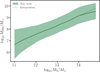 |
Fig. A.1. Relation between the halo mass and MBH mass at redshift z = 0. |
All Tables
All Figures
|
Fig. 1. Evolution of the luminosity function. In green, we show the prediction of our model when fitting for the LF itself at redshifts 0.25, 0.5, 3 and 6, as well as for the GW background measured by EPTA, displaying the median (green line) and 90% confidence interval (green band). This should be compared with the fits to the observed LF from Lacy et al. (2015) (pink) and Shen et al. (2020) (purple) and the region in between (light pink), where we allow the observed LF to lie in our likelihood. At redshifts z = 4, 5 we also plot constraints from JWST (squares) from Matthee et al. (2024). The lowest luminosity point is shown in grey and not in black, because it is likely affected by incompleteness (see the discussion in Matthee et al. 2024). At redshift z = 7, we plot a lower bound obtained by Greene et al. (2024) using JWST results. |
| In the text | |
|
Fig. 2. Stochastic GW background predicted by our model (green) and the free spectrum measured by EPTA (blue). The 90% confidence intervals centred at the median for the amplitude of the GW background in the first and last bins, i.e., at frequencies 1/(10 yr) and 1/(1 yr), are |
| In the text | |
|
Fig. 3. Relation of the stellar mass and MBH mass at redshift z = 0. We compare our results, in green, with the fit of the local relation from Greene et al. (2020) (‘all’), in blue, and the data also compiled in Greene et al. (2020), in black. Green points show a (random) subsample of MBHs produced in our simulations. |
| In the text | |
|
Fig. 4. Relation of the MBH mass and stellar mass at redshift z = 3, 4, 5, and 6. The darker green regions represent our results when restricting to MBHs with luminosity larger than 1011 L⊙, in order to mimic selection effects at high redshift. For z = 4, 5 and 6, we show JWST observations in the redshift range z = 4 to 7 (Maiolino et al. 2024; Übler et al. 2023; Harikane et al. 2023; Li et al. 2025a), some of which were used to obtain the fit of Pacucci et al. (2023) (light orange, excluding the more recent data of Li et al. 2025a). For comparison, we also show the fit to the observed local relation (light blue) of Greene et al. (2020). |
| In the text | |
|
Fig. 5. Posterior on the model parameters related to seeding and BH mergers when fitting for the LF and GW background. We show the mean and standard deviation of the log-normal distribution of seed BH masses, μseed and σseed; the minimum mass of haloes seeded Mh, seed and the seeding probability fseed; the delay of binary BH mergers (in addition to halo dynamical friction), tdelay. |
| In the text | |
|
Fig. 6. Posterior on the model parameters related to accretion when fitting for the LF and the GW background. We show the slope of the power-law distribution γburst and the duration tburst of burst accretion; the mean and standard deviation of the log-normal distribution of steady accretion rates, μsteady and σsteady; the redshift zcut below which accretion is shut off for heavier MBHs; the slope of the increase of the shut-off mass, mcut, 0 at z = 0, with redshift, αcut. |
| In the text | |
|
Fig. 7. Prediction of the yearly rate of MBH mergers after fitting for the LF and the GW background measured by EPTA. The solid curve shows the intrinsic rate, the dotted one the rate of detetable events, assuming an S/N threshold of 10. For comparison, we also report the predictions for the intrinsic rate of other models from the literature (see text for description). For Q3-nod, Q3-d and PopIII-d, the shaded areas show the range reported in reference Barausse et al. (2023) (the lower bound corresponding to finite resolution results, and the upper bound to results extrapolated to infinite resolution). For model HS-nod-SN-high-accr, we only report finite resolution results (i.e. a lower bound) as the extrapolation was not provided in reference Barausse et al. (2023). |
| In the text | |
|
Fig. 8. Prediction of the yearly rate of mergers as a function of the total source-frame mass of the binary. Thick lines show the median and shaded areas the 90% confidence region after fitting for the LF and the GW background of EPTA. The green curves correspond to the intrinsic merger rate, while the light green curves show the rate of events detectable by LISA, assuming an S/N threshold of 10. Predictions from other models are included for comparison. |
| In the text | |
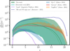 |
Fig. 9. Prediction of the yearly merger rate as a function of the redshift (see also Fig. 8). |
| In the text | |
|
Fig. A.1. Relation between the halo mass and MBH mass at redshift z = 0. |
| In the text | |
Current usage metrics show cumulative count of Article Views (full-text article views including HTML views, PDF and ePub downloads, according to the available data) and Abstracts Views on Vision4Press platform.
Data correspond to usage on the plateform after 2015. The current usage metrics is available 48-96 hours after online publication and is updated daily on week days.
Initial download of the metrics may take a while.