| Issue |
A&A
Volume 700, August 2025
|
|
|---|---|---|
| Article Number | A36 | |
| Number of page(s) | 20 | |
| Section | Stellar structure and evolution | |
| DOI | https://doi.org/10.1051/0004-6361/202453607 | |
| Published online | 31 July 2025 | |
Red supergiant stars in binary systems
II. Confirmation of B-type companions of red supergiants in the Small Magellanic Cloud using Hubble ultraviolet spectroscopy
1
Centro de Astrobiologia (CAB), CSIC-INTA, Carretera de Ajalvir km4, 28850 Torrejón de Ardoz, Madrid, Spain
2
Instituto de Astrofísica de Canarias, E-38205 La Laguna, Tenerife, Spain
3
Argelander-Institut für Astronomie, Universität Bonn, Auf dem Hügel 71, 53121 Bonn, Germany
4
Max-Planck-Institut für Radioastronomie, Auf dem Hügel 69, 53121 Bonn, Germany
5
Department of Physics and Astronomy, Johns Hopkins University, 3400 N. Charles Street, Baltimore, MD 21218, USA
6
Departamento de Física Aplicada, Universidad de Alicante, E-03690 San Vicente del Raspeig, Alicante, Spain
7
Universidad Europea de Canarias, La Orotava, Tenerife, Spain
⋆ Corresponding author: This email address is being protected from spambots. You need JavaScript enabled to view it.
Received:
24
December
2024
Accepted:
29
April
2025
Abstract
Red supergiant (RSG) stars represent the final evolutionary phase of the majority of massive stars and hold a unique role in testing the physics of stellar models. Eighty-eight RSGs in the Small Magellanic Cloud (SMC) were recently found to have an ultraviolet (UV) excess, which was attributed to a B-type companion. We present follow-up Hubble Space Telescope (HST) UV (1700–3000 Å) spectroscopy for 16 of these stars to investigate the nature of the UV excess and confirm the presence of a hot companion. In all cases, we are able to confirm that the companion is a main-sequence B-type star based on the near-UV continuum. We determine effective temperatures, radii, and luminosities from fitting the UV continuum with TLUSTY models and find stellar parameters in the expected range for SMC B-type stars. We display these results on a Hertzsprung–Russell diagram and assess the previously determined stellar parameters using UV photometry alone. From this comparison, we conclude that UV photometric surveys are vital to identify such companions and that UV spectroscopy is similarly vital to characterise the hot companions. From a comparison with IUE spectra of 32 Cyg, a well-known RSG binary system in the Galaxy where the companion is embedded in the wind of the RSG, four targets display evidence of also being embedded in such a wind. The ages of seven targets, determined via the stellar parameters of the hot companions, are found to be in tension with the ages determined for the RSG. An explanation for the discrepancy could be unaccounted for binary mass-transfer or red straggler stars.
Key words: binaries: general / stars: massive / supergiants / Magellanic Clouds
© The Authors 2025
 Open Access article, published by EDP Sciences, under the terms of the Creative Commons Attribution License (https://creativecommons.org/licenses/by/4.0), which permits unrestricted use, distribution, and reproduction in any medium, provided the original work is properly cited.
This article is published in open access under the Subscribe to Open model. This email address is being protected from spambots. You need JavaScript enabled to view it. to support open access publication.
1. Introduction
Red supergiant (RSG) stars are the final evolutionary phase of the majority of massive stars before they undergo core-collapse supernovae. Hydrogen-rich Type II-P supernovae are the most commonly observed type of core-collapse supernova, and theory and observations agree that RSGs are most frequently the progenitor stars. The observed mass distribution of Type II-P supernova progenitors display a dearth of systems more massive than around 17–20 M⊙ (Smartt 2009), although see Beasor et al. (2025) for a statistical assessment. This can be interpreted as evidence that more massive stars transition through the RSG phase and explode at a different evolutionary phase. The properties of observed populations of RSGs are sensitive tests to these evolutionary models. Models predict that at certain masses and metallicities after the RSG phase, stars evolve bluewards on the Hertzsprung–Russell diagram (HRD) and reside in the yellow or blue supergiant regime (e.g. Ekström et al. 2012; Schootemeijer et al. 2019). There is some observational support for this based on mass-loss rates of yellow supergiants (e.g. Humphreys et al. 2023). However, recent results from the Binary at LOw Metallicity (BLOeM) campaign (Shenar et al. 2024) targeting the Small Magellanic Cloud (SMC) indicate that the multiplicity statistics of BAF-type supergiant stars are inconsistent with those of RSGs (Patrick et al. 2025), which calls into question an evolutionary connection between these phases.
The role of binary evolution in this picture is clearly significant, but the multiplicity properties for RSGs are currently not well constrained. Multiplicity among main-sequence massive stars is observed to be almost unity (Sana et al. 2012; Kobulnicky et al. 2014; Moe & Di Stefano 2017), and the observed distributions of orbital parameters dictate that, as stars evolve off the main sequence, they frequently exchange mass with a close companion (de Mink et al. 2014). Such mass-transfer events are expected to result in stripped envelope stars rather than RSGs (Eldridge et al. 2008). Stars in binary systems that are close enough to merge produce rejuvenated projects that can subsequently evolve to the RSG phase (e.g. Schneider et al. 2019). Such a merger is the current best explanation for the progenitor of SN1987A (Podsiadlowski et al. 1992; Menon & Heger 2017), which likely spent a significant fraction of its post-main-sequence lifetime as a RSG, potentially with a hot companion, before eventually merging (Podsiadlowski et al. 1992). This scenario also plays an important role in explaining the observed population of blue supergiants (Menon et al. 2024). Evidence of these so-called red straggler stars in the RSG phase is best observed in the luminosity distribution of young massive star clusters (Beasor et al. 2019; Britavskiy et al. 2019; Patrick et al. 2020; Wang et al. 2025), which are estimated to account for up to 50% of the RSGs in clusters (Britavskiy et al. 2019; Patrick et al. 2020).
Identifying and characterising the population of RSGs currently in binary systems is key to understanding the RSG population as a whole. The known population of RSGs in binary systems is around 20% (Neugent et al. 2020; Patrick et al. 2022), and the orbital period distribution is poorly characterised in general, with orbital periods known for only around ten systems (Patrick & Negueruela 2024, and references therein). Of these systems, the majority of companions are B-type main-sequence stars and the orbital periods range from around 1000 d to 100 yr. These systems are frequently found to display evidence of interaction between the companions. This interaction is typically assumed to be between the wind of the RSG and the hot companion, and the evidence of this is circumstellar emission lines seen in the ultraviolet (UV; Kudritzki & Reimers 1978). In the case of the eclipsing binaries VV Cep (Wright 1977) and KQ Pup, the hot companions are embedded in a dense circumstellar material.
The population of such well-understood RSG binaries in the Milky Way is so small that it is unclear if selection biases play a role in their detection. Despite this, this population serves to guide expectations. B-type main-sequence stars are the most common companions (see e.g. Pantaleoni González et al. 2020) in the Milky Way population; other companions include a RSG+neutron star system (Masetti et al. 2006; Hinkle et al. 2020; Patrick & Negueruela 2024) and a potential RSG+RSG/YHG system (Wittkowski et al. 2017). Since the early work of Burki & Mayor (1983) on the Milky Way, populations of RSG binary systems have been discovered in galaxies in the Local Group (Neugent et al. 2020; Neugent 2021; Patrick et al. 2022; and see Patrick et al. 2024 for a review of such studies).
In Patrick et al. (2022; henceforth Paper I), we studied the UV properties of RSGs in the SMC using Ultra-Violet Imaging Telescope (UVIT) ASTROSAT photometry and discovered that 88 stars present a UV excess, which we attributed to the presence of a binary companion. In this paper, the second in the series, we follow up on a fraction of these companions with Hubble Space Telescope (HST) UV spectroscopy with the aim of confirming the nature of the targets and better characterising the binary systems. The sample selection and HST observations are described in Sect. 2. Section 3 presents the key results, including stellar parameters determined from UV continuum fitting and results from the spectral energy distribution (SED) analysis. These results are discussed in Sect. 4 and placed in the context of previous results from Paper I. Finally, we conclude this article in Sect. 5.
2. Observations
2.1. Sample selection
The sample was selected to focus on the highest likelihood RSG binary systems in the SMC. All targets were required to have a clear UV-detection from the UV imaging survey of the SMC (Thilker et al., in prep.). Thilker et al. conducted a far-UV photometric survey of the SMC using the UVIT on board the ASTROSAT satellite. The survey consists of over 30 fields covering roughly 2/3 of the footprint of the SMC at a depth of 20.3 AB mag at 1700 Å. The spatial resolution of the instrument is around 1″, which affords a significant improvement in photometric precision over GALEX and Swift surveys. In this sense, the majority of the targets have been previously identified as RSG binary systems in Paper I and have tentative stellar parameters determined using UV photometry alone. In addition, targets with radial velocity variability from Dorda & Patrick (2021; henceforth DP21) were prioritised, which allows us to focus on the systems with the smallest separation.
DP21 flagged LHA 115-S 7 as the most radial velocity (RV) variable star in their sample and, hence, a likely RSG binary system. However, this source is not included in the study of Paper I as it is not in the RSG parent catalogue of Yang et al. (2019). By cross-matching the coordinates of the cool component with the UVIT SMC survey of Thilker et al (in prep.), we find that the UV-bright component is almost one magnitude brighter in the far-UV than any of the companions identified in Paper I. Therefore, we included this target in the sample for spectroscopic follow-up. In total, 28 targets were selected for follow-up observations.
2.2. New Hubble STIS spectra
As part of the Cycle 29 HST SNAP programme (16776; PI: L. Patrick), of the 28 proposed targets we observed 16 RSGs with hot companions. The spectral types for the RSG primaries, together with their stellar parameters, which were determined in Paper I are listed in Table 1. The Sanduleak (1989) KM-star catalogue of the SMC is used as the naming convention for sources in this article.
Spectral types, IDs, and stellar parameters of the RSG components of the systems.
The targets were observed using the Space Telescope Imaging Spectrograph (STIS) with the CCD G230LB configuration to obtain spectra covering the range 1685–3065 Å with a spectral resolving power (R) of ∼700. We used the 52 × 0.2E1 pseudo-aperture resulting in a 0.2″ slit width at a favourable position on the detector. Target acquisition focused on the RSG star and the exposure time was determined on a star-by-star basis. Acquisition images used the F28X50LP aperture with the long-pass filter, which has a pivot wavelength of 7229 Å and full width at half maximum of 2722 Å. On visual inspection of these images, there were no other sources in any of the 5 × 5″ field of view images that contaminated the near-UV spectra and each target is point-like and displays no obvious signs of blurring from a nearby source, which could be the source of the UV flux. Despite the broad, red filter used in the acquisitions, tests with the STIS exposure time calculator demonstrated that an early B-type star would be detectable at low S/N in such acquisition images and their absence adds strength to the conclusion that the source of the UV flux is coincident on the position of the RSG. In addition, we cross-matched each source with Gaia Data Release 3 (DR3) and find no Gaia sources nearby that are bright enough to contaminate the UV spectra.
Each observation is a maximum of one full HST orbit and the signal-to-noise ratios (S/N) obtained ranged from 30 to 60 per resolution element. We selected candidates with F172M magnitudes of less than 19.8 to obtain sufficient S/N in one orbit. Data reduction and spectral extraction was carried out using the latest version of the STIS official pipeline with the most recent version of the appropriate bad-pixel mask used in all cases, which was only available around six months after observation. An analysis of the reconstructed two-dimensional spectrum shows no evidence of any additional targets in the slit. SkKM 250 is the exception to this with a faint nearby target that does not contaminate the central spectrum. The nature of this target is discussed in Appendix E.1. We tested the scattered light correction of Worthey et al. (2022) and found that the correction is typically on the < 1.0% level for our targets, but can reach up to 8% in some cases. Correcting for this effect does not alter the spectral appearance, nor any individual feature, but rather changes the continuum distribution, which may affect the model fitting analysis if left uncorrected. Upon testing, it was clear that the scattered light correction is well within the uncertainties of the model fits.
In general, the overall spectral appearance of the targets are consistent with a normal B-type star with several interstellar lines overlaid (more details are given in Sect. 3), which is characteristic of the SMC. There are several examples of bad pixels that were not corrected by the final version of the bad-pixel mask for each observation, the most pronounced of which was at around 2900 Å, present in all of the spectra. We removed any remaining bad pixels on a case-by-case basis in the final spectra.
2.3. UV photometry
By design, the sample have UV photometry from the UVIT SMC survey (Thilker et al., in prep.). To aid the characterisation of the hot companions we utilised point spread function (PSF) fitting photometry as part of the Swift Ultraviolet Survey of the Magellanic Clouds (SUMaC; Hagen et al. 2017). SUMaC observed all targets in three photometric filters, namely, uvw2, uvm2, and uvw1, which have a PSF full width half maximum of 2.92, 2.45, and 2.37″ and central wavelengths of 1928, 2246, and 2600 Å, respectively. Further details of the survey are given in Hagen et al. (2017). Such photometric observations are an excellent complement to data from the UVIT SMC survey.
By cross-matching our catalogue with the PSF photometry of Hagen et al. (2017), we found that 14/16 of the observed sample have Swift photometry in all three photometric bands. The two stars without Swift photometry (SkKM 310 and 320) fall outside the field of view of the SUMaC survey. The two wider Swift filters (uvw1 and uvw2) have a known red-leak, which results from the shape of the filter throughout profile and effectively allows bright red objects to contaminate the UV photometry. This is a particular consideration for our targets as, by construction, these sources have a bright red companion. The third Swift filter, uvm2, is sufficiently narrow that the filter does not suffer from the red leak problems. After tests with the photometry we only considered targets to have a meaningful detection of a binary companion if the source has a consistent detection in the uvm2 filter. All of the observed targets have uvm2 data consistent with both the other Swift filters and the UVIT detections from Paper I.
2.4. Visual data
As noted above, the targets were selected for follow-up based on the availability of multi-epoch RV observations from DP21, which probe the orbital motion of the RSG. We cross-matched the 16 targets with Gaia DR3 and found good matches to within 1″ for all targets. Gaia DR3 provides additional RV information for 15/16 of the targets. A characterisation of the orbital configuration based on the RV curves of the systems remains, unfortunately, beyond the reach of currently available observations as a result of the combination of sparse RV sampling and long suspected orbital periods.
Table 2 provides a summary of the available RV information for each target. A comparison of the peak-to-peak RV (Δv) from DP21 and that of Gaia DR3 shows that there is an inconsistency between the two measurements. The Gaia DR3 Δv measurement has no associated uncertainty but based on tests for the wider RSG population of the SMC, we assumed that there is a systematic uncertainty associated with these measurements. To solve this requires Gaia DR4. We retain this information in Table 2 to serve as a comparison, but do not consider it further in the text. That being said, the difference for LHA 115-S 7 is puzzling. One would assume that for large values of Δv the Gaia data would be reliable. Interestingly, if we exclude Gaia DR2 from the measurements of DP21, we find Δv = 10 km s−1, which is consistent with the Gaia value. In addition to the systematic uncertainty discussed above, we consider it possible that there is a discrepancy between the Gaia and non-Gaia RVs for this source.
RV information for the targets.
In addition, we compiled photometric observations from the visual to the infrared from various sources to determine the SED of the RSG component and determine stellar parameters. Finally, none of the targets were classified as binary with the Gaia DR3 NON_SINGLE_STAR flag. This flag identifies astrometric binaries and spectroscopic binaries; therefore, an expectation here may have been that some RSG binaries were picked up by the spectroscopic binary flag given that an excess is observed in the Gaia XP spectra.
3. Results
From the HST/STIS spectra all sources display a UV continuum consistent with a B-type star. Based on this result, combined with the consistency of the positions of the UV source and the RSG component from Paper I and the statistically insignificant possibility that a chance alignment occurs to such a high spatial accuracy (e.g. Neugent et al. 2020; Bianchi 2024), we conclude that the stars form physically associated binary systems. A montage of the spectra is shown in Fig. 1. Four sources SkKM 108, 209, 286 and 320 show departures from a normal B-type star continuum, this is discussed further in Sect. 4.3.
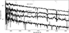 |
Fig. 1. Montage of the observed HST/STIS UV spectra. Each spectrum has a S/N per resolution element of at least 30 at ∼2400 Å, ranging to ∼60 for LHA 115-S 7. The flux distribution is not normalised, to enable a better visualisation of the hot star continuum. Line identifications are marked in grey; however, we note that the only features detectable in the spectra are of interstellar origin and not suitable for stellar parameter determination. No normalisation factor is applied to any of the spectra displayed here. All 16 spectra are shown individually in Appendix A. |
To test whether the RSG component contaminates the STIS spectra, we exploited the HST ASTRAL spectral database (Ayres 2014) and rescaled the spectra of α Ori (M2 Ia) and β Gem (K0 III) to match the V-band magnitude of each target individually. From this comparison in no cases would a star like α Ori contaminate the spectra and only in three cases does the K0 star β Gem have sufficient flux to potentially contaminate the near-UV spectrum: SkKM 171, 239, and 310. However, none of these targets, nor any others display clear signs of contamination from the RSG component. This is supported by the SED fitting analysis below.
3.1. Stellar parameters from UV continuum fits
To determine stellar parameters of the hot component, we used model spectra from the TLUSTY SMC BSTAR and OSTAR grids with effective temperatures covering the range 15 000–55 000 K (Lanz & Hubeny 2003, 2007). These spectra were convolved with the STIS G230LB line spread function andre-binned the STIS CCD pixel size, corrected for extinction (discussed below), and fitted to each spectrum to yield an angular radius and a χ-squared value based on the observed flux errors in each pixel. An example fit is show in Fig. A.1. Given the modest resolution of these data, stellar rotation was ignored. The low resolution of the data precludes the use of stellar absorption lines in determining spectral types, the strong lines that are present are dominated by their interstellar contribution. Unfortunately the Fe III complex of lines in the vicinity of ∼1900 Å that is characteristic of early B-type stars, lies at the blue edge of the G230LB spectral range where uncertainties are large, and hence this feature provides little leverage on the fit. The overall goodness of fit is therefore largely driven by the slope of the near-UV continuum, the best fitting model being determined by the minimum χ-squared value for the grid of models. The stellar radii and luminosities follow from the assumed distance to the SMC (dmSMC = 18.977; Graczyk et al. 2020). Including the UVIT and Swift photometry to help constrain the fit is not useful as these data provide no additional wavelength coverage and often display a flux offset (see Appendix A).
Correction for extinction is a critical input to the fit process. However, experimenting with treating this as a variable (cf. Gordon et al. 2024) with just the near-UV bandpass proved unsuccessful. Additional longer wavelength data are unsuitable for constraining the extinction because of contamination from the RSG component. Wang & Chen (2023) provide individual values of extinction parameters for eight of the stars in this sample based on a measurement of an intrinsic colour of RSGs as a function of effective temperature. Based on the analysis presented in Appendix B, we decided not to use these measurements as a result of their underestimated intrinsic uncertainty and the lack of correlation with the Ks − [24 μm] colours. We therefore opted to use a mean value of the extinction that we determined from a sample of 321 O-type stars with literature spectral types, taken mainly from Bonanos et al. (2010). O-type stars are ideal diagnostics of extinction as their B − V intrinsic colour is almost degenerate with spectral type and metallicity (Lanz & Hubeny 2003). The B − V colours for the O-star sample were determined from their Gaia XP spectra, and intrinsic colours were taken from Wegner (1994) to infer a mean of E(B − V) = 0.08 with standard deviation 0.06. Following Gordon et al. (2024), we assumed 0.04 magnitudes of foreground Milky Way extinction, and 0.04 magnitudes of SMC extinction, with appropriate average extinction laws. The individual values of the E(B − V) for the targets are listed in Table B.1 for comparison.
In general it was found that surface gravities in the range log g = 3.5 − 4.5 gave similar quality fits, with lower surface gravities being significantly worse in this regard. However, the G230LB data offer little leverage to refine this rough estimate and hence we do not report explicit values of log g other than to note that the sample is consistent with being on the main sequence. An additional caveat concerns the effective temperatures. For values close to, or above, 30 kK the upper bound is poorly constrained as the continuum slope becomes insensitive at higher effective temperatures. At the cooler end of the scale we note that 15 kK is the lower bound on the model grid, although the fits for the three stars with values near this edge appear reasonable (SkKM 239, 310, and 320).
The results of this fitting using a fixed E(B − V) = 0.08 are shown in Table 3. In addition, Fig. 2 displays the stellar parameters graphically on a HRD, which also shows stellar tracks of different ages. To assess the uncertainties on the fits, we repeated this fitting process with a different model grid, that of the ATLAS9 models from Howarth (2011), with a range of different assumptions. The uncertainties listed in Table 3 reflect the distribution of resulting parameters. In most cases the fits are robust to varying logg in the range 3.0 < log g < 5.0 and assuming a range of E(B − V) values. This includes the sources at the low edge of the effective temperature grid, and in addition, we find no evidence that the four stars labelled ‘embedded’ in Sect. 4.3 have poorer fits.
The effective temperatures span the full range of the grid from 15 − 35 kK with luminosities in the range 3 < log L/L⊙ < 5. LHA 115-S 7, has the most luminous companion. Excluding this star the luminosity distribution peaks at log L/L⊙ = 4.4. This distribution of luminosities and effective temperatures is in good agreement with the known population of B-type main-sequence stars in the SMC. When displayed on the HRD in Fig. 2, there appears to be two groups of targets, a low-luminosity group with effective temperatures of less than 18 kK and luminosities of less than log L/L⊙ = 3.5 and a higher-luminosity group with 4.0 < log L/L⊙ < 4.5. Such a distinction is unexpected given the roughly continuous distributions of UVIT F172M magnitudes, luminosities and effective temperature of the companions although small number statistics prevents any conclusions from being drawn from such an apparent bimodal distribution.
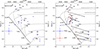 |
Fig. 2. Left: HRD for the 16 targets with stellar parameters determined from the G230LB STIS spectra, shown as blue stars. The blue point shows the typical uncertainties on the stellar parameters (see Section 3.1 for more details and caveats). The grey lines show SMC stellar tracks using a mass-dependent overshooting parameter (Schootemeijer et al. 2019; Hastings et al. 2021), where dashes are marked at intervals of 0.05 Myr. The dashed lines show isochrones of ages 10, 20, and 30 Myr. Spectral types for SMC dwarf stars are shown using the calibration presented in Shenar et al. (2024). Large black circles mark the stars labelled ‘embedded’ in Table 3. Right: Same as the left panel but we add the stellar parameters determined from Patrick et al. (2022) in red. The uncertainties are illustrated with the red point. Black lines connect the stellar parameters derived using the two methods. |
3.2. Spectral energy distributions
We determined effective temperatures and radii of the RSG component from SED fitting of photometry, assuming a distance modulus to the SMC (dmSMC = 18.977; Graczyk et al. 2020). The photometry is compiled from Gaia DR3 and the Two Micron All-Sky Survey (Skrutskie et al. 2006) and in the fitting procedure the photometry is weighted by their respective uncertainties. Figure 3 illustrates an example fit. An examination of these fits, which are shown in Appendix C, reveals that in all cases the flux contribution from the RSG component is negligible in the near-UV spectral range, in good agreement with the ASTRAL analysis. In addition, these figures reveal that the nature of the hot companion is uniquely revealed by the near-UV spectra. The U-band in some cases shows evidence of contamination from the hot companion, but is in all cases fit reasonably well with a single RSG SED.
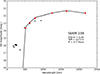 |
Fig. 3. Example of the SED fitting to determine the stellar parameters of the RSG component. The large red points are from Gaia and 2MASS and are the only photometry given weight in the fit. Black points are from Skymapper, Swift, and UVIT. |
Stellar parameters are determined using the best-fit Castelli & Kurucz model atmospheres to the V- through K-band photometry assuming a fixed surface gravity of log g = 1.0 and metallicity of Z = 0.002 or 14% solar, which is typical of the SMC, and an SMC-like extinction curve. We compared the stellar parameters from the SED fitting and find very good agreement in general. For all stars apart from LHA 115-S 7, the agreement is well within assumed uncertainties on the individual parameters. The median difference between the effective temperatures is ±60 K and ±0.03 dex in luminosity. In general, the fitting process prefers very low reddening values, which leads to E(B − V) = 0.0 in some cases. Repeating this process with a different extinction law improves the fit in some cases but the reddening values remain small. The change to the stellar parameters is minimal. From this analysis we conclude that the E(B − V) values are relatively poorly constrained from our fits, but low E(B − V) are in general preferred. Comparing these results to the adopted E(B − V) values from the OB-type star comparison shows no obvious trend.
The stellar parameters for LHA 115-S 7 are not well fit, which is likely the result of the prominent Hα emission feature perturbing the fit. Repeating the fits using different reddening, log g and metallicity values illustrate that the stellar and extinction parameters are poorly constrained for this source. Stellar parameters determined from Apache Point Observatory Galactic Evolution Experiment (APOGEE) data for this star (Abdurro’uf et al. 2022) result in Teff = 4278 K, which is in good agreement with the effective temperature determined using the analysis of Paper I. However, the E(B − V) value from APOGEE is considerably larger than the values from the fitting routine and from the OB-star analysis.
4. Discussion
4.1. Comparison with stellar parameters from single epoch photometry
In Paper I we determined stellar parameters for the hot stars by making three simplifying assumptions, the first is that the hot star is a main-sequence star, the second is that the age of the hot companion is the same as the RSG and the third is the extinction parameters are same for the two components. With the results presented for the HST near-UV spectra in Sect. 3, we are able to assess some of these degeneracies and improve upon the earlier measurements, in terms of both accuracy and precision. Figure 2 shows a direct comparison between the stellar parameters determined in Paper I and those determined here.
In 10/16 stars the effective temperature is significantly smaller than determined in Paper I and in all cases the luminosity determined is smaller than those in Paper I. For the six stars that have higher effective temperatures from the HST/STIS spectra, the difference is significant only for the two hottest stars where it is likely that the uncertainties are underestimated. To test whether the difference in stellar parameters is the result of a discrepancy between the HST spectra and the UVIT photometry we compute synthetic photometry in the UVIT far-UV band from the HST/STIS spectra. On average the UVIT observations are consistent with the HST/STIS spectra to within a standard deviation of ±0.4 mag, which is larger than expected. The origin of such large discrepancies is unclear but may be the result of inaccurate absolute flux calibration of the UVIT observations or potentially inaccuracies in the centring of the target on the slit in the HST/STIS spectra. If we recompute the stellar parameters using the synthetic UVIT observations with the same routines as in Paper I, we find that the effective temperatures are always within the uncertainties but are usually between 0 and 400 K warmer. Similarly, the luminosities are typically within ±0.15 dex in all but two cases. Based on this analysis, we rule out the possibility that the differences between the determined stellar parameters from the UVIT and HST data are the result of differences in the flux calibration between the two datasets. The differences therefore may represent genuine intrinsic variability or inaccuracies in the model fitting procedure. This can be further assessed with additional spectra of the hot component.
4.2. Are the ages of the two components consistent?
In Paper I we concluded that the majority of the targets (including 15/16 of the targets in this study) were consistent with the assumption of having coeval components. Only six targets from Paper I displayed observations that were clearly inconsistent, which resulted in a mass-ratio (q = mB/mRSG) greater than 1. LHA 115-S 7 was not in the sample of stars studied in Paper I, but by determining the stellar parameters for both components using the same analysis routines, we found that this system also has q > 1. Perhaps the most important consequence of revising the stellar parameters of these stars is the realisation that the hot companions are, in general, significantly older and less massive than assumed in Paper I.
In Paper I we determined ages for the RSG component via a comparison with the same stellar evolutionary models as used in this study. To do this, we determined a calibration between the RSG luminosity and the mid-point of the core-helium burning sequence in the models. While this assumption is simplistic, at 8 M⊙ the star spends only 1.6 Myr in the RSG phase and throughout this time the luminosity is roughly constant. This illustrates that even if the RSG is more or less evolved than expected, the determined age would not be significantly affected. Based on this, we conclude that this assumption provides a realistic estimate of the age of star, although this neglects the fact that at the very end of their lifetimes RSG ages are very uncertain (e.g. Farrell et al. 2020). We then used the age determined for the RSG from this analysis, combined with the UVIT magnitude, to determine the stellar parameters of the B-type star from the models.
In this study, we determined the ages for the hot companions independently of the RSG by comparing their stellar parameters – determined using the methods described in Sect. 3 – to the models. For these measurements we assumed uncertainties of ±5 Myr as a conservative estimate to take the uncertainty in logg into account. Figure 4 compares the ages determined from the stellar parameters of the hot companions with those of the RSGs from Paper I. The ages for the 16 RSGs range between 12 and 22 Myr with uncertainties between ±2 and 3.5 Myr, which increases as a function of the determined age. In contrast, the ages of the hot companions are in the range 0–120 Myr. The majority of the hot companions show ages broadly consistent with that of the RSGs. However, for seven sources the ages of the RSG is in clear tension with that of the hot companions: five stars display ages too old and two appear too young to host a RSG companion. We experimented with different stellar models from Schootemeijer et al. (2019), assuming different mixing parameters with convective overshooting ranging between 0.11 and 0.55. A larger convective overshooting parameter extends the main sequence to cooler effective temperatures but does not relieve the tension between the ages of the two components. This is because, a seven solar mass model, for example, spends the first 40 Myr the very close the position of the zero age main sequence regardless of the assumed mixing parameters.
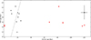 |
Fig. 4. Comparison of the ages of the hot companions (abscissa) and the RSG components (ordinate) of the 16 binary systems studied. The dashed grey line shows the expectation of coevality, i.e. a one-to-one relationship. The ages of the two components are inconsistent in seven of the 16 cases at the ∼3σ level. These sources are marked with red stars. The black point on the left indicates the typical uncertainties. |
Our conclusion is that for 7/16 sources some form of binary evolution must have taken place in order to explain the apparently different ages of the two components. We rule out the scenario that the two stars are not physically associated based on arguments presented at the beginning of Sect. 3. Interestingly, to the authors knowledge, there are no cases of a tension between the ages of different components in the Galactic population of RSG binary systems.
For the five older B-type stars, an explanation for the age discrepancy are ‘red straggler stars’ (Britavskiy et al. 2019). This would imply that these systems were originally in hierarchical triple systems where the inner binary has interacted, merged, and subsequently evolved to the RSG phase. In this scenario, the age of the B-type star (the original outer tertiary component) would represent the true age of the system and the RSG is the component that now appears younger because of a stellar merger.
4.3. Evidence of interactions
Four targets stand out as displaying an apparent second component in the HST/STIS spectra. This manifests as broad emission features in the near-UV continuum, the strongest of these at ∼2750 Å. The targets that display such features are SkKM 108, 209, 286 and 320. Figure 5 shows SkKM 209 and 286, along with two comparison stars, to illustrate this effect. This behaviour is not expected in normal B-type stars.
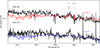 |
Fig. 5. Two examples of HST/STIS G230L spectra that deviate from a normal B-type star continuum. This behaviour is observed in SkKM 108, 209, 286, and 320 (209 and 286 shown in this figure). The red spectrum shows an IUE spectrum of 32 Cyg published in Che et al. (1983) at an orbital phase of 0.7. The blue spectrum shows an example of a normal B-type spectrum of Alpha Sco B from unpublished IUE data retrieved from the INES database (programme ID LGLMS; PI: M. A. Smith), which highlights the differences observed. Note that as the comparison stars (Alpha Sco B and 32 Cyg) are both galactic stars, the flux distribution bluewards of ∼2500 Å is different as a result of the differing extinction laws in the two galaxies. Line identifications are shown in grey. We note that in the SMC spectra the Mg II feature is dominated by the interstellar component. |
From a comparison with stars in the ASTRAL database in Sect. 3 and via the SED fitting presented in Sect. 3.2, we show that the RSG does not contaminate the near-UV continuum in any cases, even for the mid-G-type supergiant LHA 115-S 7. We therefore rule this out as a possible origin of the second component in the spectra.
To understand the origin of these features, we compared the observed spectra with archival International Ultra-violet Explorer (IUE) observations. We compared the HST/STIS spectra with various RSG binary systems in the Galaxy with main-sequence B-type star companions (see Patrick & Negueruela 2024, for a summary of the orbital parameters), as well as with single B0V – B3V stars. To do this, we used the IUE INES archive and downloaded spectra at various orbital phases for VV Cep, 22 Vul, 31 Cyg, 32 Cyg, HR6902, and ζ Aur. These spectra were then degraded to the resolving power of the G230L spectra to aid a visual comparison to the observed features in the HST/STIS spectra. From these comparisons we find that three spectra of 32 Cyg provide the best match. These spectra were observed on 30 January 1980, 4 May 1980, and 1 August 1980 at an orbital phase of 0.62, 0.7, and 0.78, respectively (Che et al. 1983), with the spectrum at the orbital phase of 0.7 matching the most closely. Spectra of 32 Cyg at other orbital phases do not show the same features observed in the HST/STIS spectra; they instead more closely resemble those of normal B-type stars. There are some similarities in the shape of the emission feature at 2750 Å with the IUE spectra of VV Cep from 4 October 1997, 16 June 1997, and 21 August 1997, but here the agreement is clearly poorer, in particular with the Mg II lines being blended into a strong emission profile in the VV Cep spectra and a general lack of agreement with the shape of the near-UV continuum.
Figure 5 also shows the closest matching IUE spectrum of 32 Cyg are observed on the 04/05/1980. We argue that this comparison shows that the spectra of these four stars can potentially be explained by the same mechanism that produces the spectrum of 32 Cyg. Stencel et al. (1979) first identified P Cygni line profiles in the Fe II and Mg II lines (among other elements), which is evidence that the hot star is embedded in the wind of the cool supergiant. Such P Cygni profiles can explain the lack of strong absorption in the Mg II interstellar lines, which is also weaker in these four sources. The hot companion of VV Cep is also embedded in the wind of the RSG, in this system; however, the emission features that dominate the spectral appearance are far stronger and bear little resemblance to what is observed in the SMC systems, which perhaps is to be expected given the significantly later spectral type of the RSG than the stars studied here. High-resolution UV spectra at multiple orbital phases are required to further this analysis, and in a third paper in this series we will assess this further. The four targets that display this behaviour are marked as ‘embedded’ in Table 3.
Stellar parameters for the hot companions to RSGs as determined by the HST/STIS Snapshot spectra.
As additional supporting evidence of the embedded interpretation, three-quarters of the embedded targets have large observed Δv values, which is indicative of orbital motion. SkKM 108 shows no evidence of orbital motion, which may indicate a significantly larger orbital period. Similar embedded spectral features are observed in the IUE spectra of α Sco, which has an orbital period of several thousand years and consequently the orbital motion displayed in this system is also very small.
Eight of the remaining objects show no indication of orbital motion and do not display evidence of interactions. This could indicate significantly larger orbital periods. However, four targets do show evidence of Δv values that are larger than expected for normal intrinsic RSG variability: LHA 115-S 7, [M2002] SMC 54134, and PMMR 61. The strong Hα emission line profile in LHA 115-S 7 is evidence of interaction, but no evidence is seen of this in the near-UV continuum as might be expected. The remaining two stars ([M2002] SMC 54134 and PMMR 61) show no evidence of interaction but display significant orbital motion, which implies shorter orbitalperiods.
5. Summary and conclusions
We have presented the analysis of HST/STIS spectra in the 1700–3000 Å spectral range for 16 RSG binary systems in the SMC that were discovered in Paper I. The aim of this study was to confirm the nature of the binary systems by determining the nature of the hot companions and assessing the simplifying assumptions made in Paper I. To do this, the observations focused on highly likely RSG binaries with observed orbital motion from DP21. Using the UV continuum from the HST/STIS spectra, we determined stellar parameters for the hot components – independently of the RSG components – via a comparison with stellar models. In addition, we compiled visual-through-infrared photometry to constrain the stellar parameters of the RSG component. Our main conclusions are:
-
According to the near-UV HST/STIS spectral appearance, all the hot companions are B-type main-sequence stars, in good agreement with expectations.
-
Stellar parameters are well determined from the current spectra. Based on TLUSTY model fits to the near-UV spectra, stellar parameters vary considerably from those determined from UV-photometry alone. In general, the companions are cooler and subsequently less luminous than what was determined in Paper I.
-
At least four systems show evidence of interaction, which – at the resolution of the HST/STIS spectra – manifests as broad emission features that deviate from the continuum expected for normal B-type stars.
To improve the accuracy of the stellar parameter results presented here, follow-up far-UV spectra are required. This will be the subject of the third paper in this series, which will use complementary HST/STIS observations. In addition, follow-up multi-epoch spectroscopic observations from the 4-metre Multi-Object Spectroscopic Telescope One Thousand and One Magellanic Cloud survey (Cioni et al. 2019), combined with Gaia DR4 and the long baseline information from DP21, may provide some constraints on orbital periods.
We note here that this value is largely inconsistent with other studies. For the SMC RV is usually in the range 2.74 < RV < 3.1.
Acknowledgments
The authors would like to thank the referee for their detailed comments which helped improve the quality of the manuscript. The authors thank Dr F. Najarro and Dr M. Garcia for helpful discussions and advice on IUE spectra. The authors thank Prof. M. Siegel for providing us with the Swift photometry. Based on INES data from the IUE satellite. LRP acknowledges support by grants PID2019-105552RB-C41 and PID2022-137779OB-C41 funded by MCIN/AEI/10.13039/501100011033 by “ERDF A way of making Europe”. LRP acknowledges support from grant PID2022-140483NB-C22 funded by MCIN/AEI/10.13039/501100011033. IN is supported by the Spanish Government Ministerio de Ciencia, Innovación y Universidades and Agencia Estatal de Investigación (MCIU/AEI/10.130 39/501 100 011 033/FEDER, UE) under grants PID2021-122397NB-C21/C22. It is also supported by MCIU with funding from the European Union NextGenerationEU and Generalitat Valenciana in the call Programa de Planes Complementarios de I+D+i (PRTR 2022), project HIAMAS, reference ASFAE/2022/017. Contributions by LB and DT to this work were supported by grant HST-GO-16776 from the Space Telescope Science Institute under NASA contract NAS5-26555. Based on observations with the NASA/ESA Hubble Space Telescope obtained at the Space Telescope Science Institute, which is operated by the Association of Universities for Research in Astronomy, Incorporated, under NASA contract NAS5-26555.
References
- Abdurro’uf, Accetta, K., Aerts, C., et al. 2022, ApJS, 259, 35 [NASA ADS] [CrossRef] [Google Scholar]
- Ayres, T. R. 2014, in Astronomical Society of India Conference Series, eds. H. P. Singh, P. Prugniel, & I. Vauglin, 11, 1 [Google Scholar]
- Bailer-Jones, C. A. L., Rybizki, J., Fouesneau, M., Demleitner, M., & Andrae, R. 2021, AJ, 161, 147 [Google Scholar]
- Beasor, E. R., Davies, B., Smith, N., & Bastian, N. 2019, MNRAS, 486, 266 [NASA ADS] [CrossRef] [Google Scholar]
- Beasor, E. R., Smith, N., & Jencson, J. E. 2025, ApJ, 979, 117 [Google Scholar]
- Bianchi, L. 2024, ApJS, 274, 45 [Google Scholar]
- Bonanos, A. Z., Lennon, D. J., Köhlinger, F., et al. 2010, AJ, 140, 416 [NASA ADS] [CrossRef] [Google Scholar]
- Britavskiy, N., Lennon, D. J., Patrick, L. R., et al. 2019, A&A, 624, A128 [NASA ADS] [CrossRef] [EDP Sciences] [Google Scholar]
- Burki, G., & Mayor, M. 1983, A&A, 124, 256 [NASA ADS] [Google Scholar]
- Che, A., Hempe, K., & Reimers, D. 1983, A&A, 126, 225 [NASA ADS] [Google Scholar]
- Cioni, M. R. L., Storm, J., Bell, C. P. M., et al. 2019, Messenger, 175, 54 [Google Scholar]
- de Mink, S. E., Sana, H., Langer, N., Izzard, R. G., & Schneider, F. R. N. 2014, ApJ, 782, 7 [Google Scholar]
- Dorda, R., & Patrick, L. R. 2021, MNRAS, 502, 4890 [NASA ADS] [CrossRef] [Google Scholar]
- Dorda, R., Negueruela, I., González-Fernández, C., & Marco, A. 2018, A&A, 618, A137 [NASA ADS] [CrossRef] [EDP Sciences] [Google Scholar]
- Drout, M. R., Götberg, Y., Ludwig, B. A., et al. 2023, Science, 382, 1287 [NASA ADS] [CrossRef] [Google Scholar]
- Ekström, S., Georgy, C., Eggenberger, P., et al. 2012, A&A, 537, A146 [Google Scholar]
- Eldridge, J. J., Izzard, R. G., & Tout, C. A. 2008, MNRAS, 384, 1109 [Google Scholar]
- Farrell, E. J., Groh, J. H., Meynet, G., & Eldridge, J. J. 2020, MNRAS, 494, L53 [NASA ADS] [CrossRef] [Google Scholar]
- González-Fernández, C., Dorda, R., Negueruela, I., & Marco, A. 2015, A&A, 578, A3 [Google Scholar]
- Gordon, K. D., Fitzpatrick, E. L., Massa, D., et al. 2024, ApJ, 970, 51 [Google Scholar]
- Götberg, Y., de Mink, S. E., Groh, J. H., et al. 2018, A&A, 615, A78 [NASA ADS] [CrossRef] [EDP Sciences] [Google Scholar]
- Graczyk, D., Pietrzyński, G., Thompson, I. B., et al. 2020, ApJ, 904, 13 [Google Scholar]
- Hagen, L. M. Z., Siegel, M. H., Hoversten, E. A., et al. 2017, MNRAS, 466, 4540 [NASA ADS] [Google Scholar]
- Han, Z., Podsiadlowski, P., Maxted, P. F. L., Marsh, T. R., & Ivanova, N. 2002, MNRAS, 336, 449 [Google Scholar]
- Hastings, B., Langer, N., Wang, C., Schootemeijer, A., & Milone, A. P. 2021, A&A, 653, A144 [NASA ADS] [CrossRef] [EDP Sciences] [Google Scholar]
- Hill, V. 1997, A&A, 324, 435 [Google Scholar]
- Hinkle, K. H., Lebzelter, T., Fekel, F. C., et al. 2020, ApJ, 904, 143 [NASA ADS] [CrossRef] [Google Scholar]
- Howarth, I. D. 2011, MNRAS, 413, 1515 [NASA ADS] [CrossRef] [Google Scholar]
- Humphreys, R. M., Jones, T. J., & Martin, J. C. 2023, AJ, 166, 50 [NASA ADS] [CrossRef] [Google Scholar]
- Jiménez-Arranz, Ó., Romero-Gómez, M., Luri, X., & Masana, E. 2023, A&A, 672, A65 [NASA ADS] [CrossRef] [EDP Sciences] [Google Scholar]
- Kobulnicky, H. A., Kiminki, D. C., Lundquist, M. J., et al. 2014, ApJS, 213, 34 [Google Scholar]
- Kravchenko, K., Chiavassa, A., Van Eck, S., et al. 2019, A&A, 632, A28 [NASA ADS] [CrossRef] [EDP Sciences] [Google Scholar]
- Kravchenko, K., Jorissen, A., Van Eck, S., et al. 2021, A&A, 650, L17 [NASA ADS] [CrossRef] [EDP Sciences] [Google Scholar]
- Kudritzki, R. P., & Reimers, D. 1978, A&A, 70, 227 [Google Scholar]
- Lanz, T., & Hubeny, I. 2003, ApJS, 146, 417 [NASA ADS] [CrossRef] [Google Scholar]
- Lanz, T., & Hubeny, I. 2007, ApJS, 169, 83 [CrossRef] [Google Scholar]
- Masetti, N., Orlandini, M., Palazzi, E., Amati, L., & Frontera, F. 2006, A&A, 453, 295 [NASA ADS] [CrossRef] [EDP Sciences] [Google Scholar]
- Massey, P., & Olsen, K. A. G. 2003, AJ, 126, 2867 [NASA ADS] [CrossRef] [Google Scholar]
- Massey, P., Silva, D. R., Levesque, E. M., et al. 2009, ApJ, 703, 420 [Google Scholar]
- Menon, A., & Heger, A. 2017, MNRAS, 469, 4649 [NASA ADS] [Google Scholar]
- Menon, A., Ercolino, A., Urbaneja, M. A., et al. 2024, ApJ, 963, L42 [NASA ADS] [CrossRef] [Google Scholar]
- Moe, M., & Di Stefano, R. 2017, ApJS, 230, 15 [Google Scholar]
- Moehler, S., Heber, U., & Rupprecht, G. 1997, A&A, 319, 109 [NASA ADS] [Google Scholar]
- Neugent, K. F. 2021, ApJ, 908, 87 [NASA ADS] [CrossRef] [Google Scholar]
- Neugent, K. F., Levesque, E. M., Massey, P., Morrell, N. I., & Drout, M. R. 2020, ApJ, 900, 118 [CrossRef] [Google Scholar]
- Pantaleoni González, M., Maíz Apellániz, J., Barbá, R. H., & Negueruela, I. 2020, Res. Notes Am. Astron. Soc., 4, 12 [Google Scholar]
- Patrick, L. R., & Negueruela, I. 2024, Bull. Soc. R. Sci., 93, 173 [Google Scholar]
- Patrick, L. R., Lennon, D. J., Evans, C. J., et al. 2020, A&A, 635, A29 [NASA ADS] [CrossRef] [EDP Sciences] [Google Scholar]
- Patrick, L. R., Thilker, D., Lennon, D. J., et al. 2022, MNRAS, 513, 5847 [Google Scholar]
- Patrick, L. R., Thilker, D., Lennon, D., et al. 2024, in Massive Stars Near and Far, eds. J. Mackey, J. S. Vink, & N. St-Louis, IAU Symposium, 361, 279 [Google Scholar]
- Patrick, L. R., Lennon, D. J., Najarro, F., et al. 2025, A&A, 698, A39 [NASA ADS] [CrossRef] [EDP Sciences] [Google Scholar]
- Podsiadlowski, P., Joss, P. C., & Hsu, J. J. L. 1992, ApJ, 391, 246 [Google Scholar]
- Prévot, L., Martin, N., Maurice, E., Rebeirot, E., & Rousseau, J. 1983, A&AS, 53, 255 [Google Scholar]
- Sana, H., de Mink, S. E., de Koter, A., et al. 2012, Science, 337, 444 [Google Scholar]
- Sanduleak, N. 1989, AJ, 98, 825 [NASA ADS] [CrossRef] [Google Scholar]
- Schneider, F. R. N., Ohlmann, S. T., Podsiadlowski, P., et al. 2019, Nature, 574, 211 [Google Scholar]
- Schootemeijer, A., Langer, N., Grin, N. J., & Wang, C. 2019, A&A, 625, A132 [NASA ADS] [CrossRef] [EDP Sciences] [Google Scholar]
- Shenar, T., Bodensteiner, J., Sana, H., et al. 2024, A&A, 690, A289 [NASA ADS] [CrossRef] [EDP Sciences] [Google Scholar]
- Skrutskie, M. F., Cutri, R. M., Stiening, R., et al. 2006, AJ, 131, 1163 [NASA ADS] [CrossRef] [Google Scholar]
- Smartt, S. J. 2009, ARA&A, 47, 63 [NASA ADS] [CrossRef] [Google Scholar]
- Stencel, R. E., Kondo, Y., Bernat, A. P., & McCluskey, G. E. 1979, ApJ, 233, 621 [Google Scholar]
- Wang, S., & Chen, X. 2023, ApJ, 946, 43 [Google Scholar]
- Wang, C., Patrick, L., Schootemeijer, A., et al. 2025, ApJ, 981, L16 [Google Scholar]
- Wegner, W. 1994, MNRAS, 270, 229 [Google Scholar]
- Wittkowski, M., Abellán, F. J., Arroyo-Torres, B., et al. 2017, A&A, 606, L1 [NASA ADS] [CrossRef] [EDP Sciences] [Google Scholar]
- Worthey, G., Pal, T., Khan, I., Shi, X., & Bohlin, R. 2022, Am. Astron. Soc. Meet. Abstr., 240, 302.03 [Google Scholar]
- Wright, K. O. 1977, J. R. Astron. Soc. Can., 71, 152 [Google Scholar]
- Yang, M., Bonanos, A. Z., Jiang, B.-W., et al. 2019, A&A, 629, A91 [NASA ADS] [CrossRef] [EDP Sciences] [Google Scholar]
Appendix A: HST spectra and spectral fitting
An example of the spectral fitting is shown in Fig. A.1, which also displays the difference between the UVIT F172M photometry determined from the HST spectrum and that of the UVIT SMC survey (Thilker et al. in prep.).
Figures A.2 – A.17 display the HST Snap spectra for all 16 targets considered in this study.
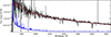 |
Fig. A.1. Example of the result of the χ-squared fitting procedure for SkKM 113. The black line shows the observed data, and the red line the best-fitting model with an effective temperature of 25kK and logg = 4.0. The red star marks the synthetic photometry in the UVIT F172M band, which was computed directly from the HST spectrum. The green star marks the UVIT F172M magnitude from Thilker et al. (in prep.). The difference in magnitude between the two is ∼0.3mag. |
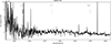 |
Fig. A.2. HST/STIS spectrum of SkKM 320. |
 |
Fig. A.3. HST/STIS spectrum of SkKM 286. |
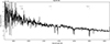 |
Fig. A.4. HST/STIS spectrum of SkKM 90. |
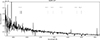 |
Fig. A.5. HST/STIS spectrum of SkKM 247. |
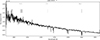 |
Fig. A.6. HST/STIS spectrum of LHA-115-S-7. |
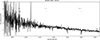 |
Fig. A.7. HST/STIS spectrum of M2002-SMC-54134. |
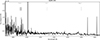 |
Fig. A.8. HST/STIS spectrum of SkKM 209. |
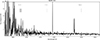 |
Fig. A.9. HST/STIS spectrum of SkKM 310. |
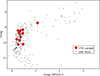 |
Fig. A.10. HST/STIS spectrum of SkKM 74. |
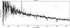 |
Fig. A.11. HST/STIS spectrum of SkKM 113. |
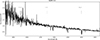 |
Fig. A.12. HST/STIS spectrum of PMMR-61. |
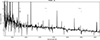 |
Fig. A.13. HST/STIS spectrum of SkKM 171. |
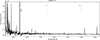 |
Fig. A.14. HST/STIS spectrum of SKKM 250. |
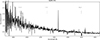 |
Fig. A.15. HST/STIS spectrum of SKKM 108. |
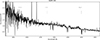 |
Fig. A.16. HST/STIS spectrum of SKKM 238. |
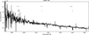 |
Fig. A.17. HST/STIS spectrum of SKKM 239. |
Appendix B: Individual extinction parameters for SMC RSGs
Table B.1 displays the reddening values determined from the 20 nearest O-type stars. See Sect. 3 for further details on this analysis. In general, the E(B − V) values are small with no examples of sources being located in regions of higher intrinsic extinction within the SMC. This gives us confidence that the assumed extinction parameters in the fits are robust.
E(B − V) values determined from the 20 nearest O-type stars.
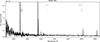 |
Fig. B.1. Ks-band magnitudes (MKs) vs Ks − 24μm colour-magnitude diagram for SMC RSGs (grey points) from Patrick et al. (in prep.). The red diamonds show RSGs observed with UV SITS spectroscopy. |
The extinction parameters derived using this method are not sensitive to circumstellar extinction intrinsic to the RSG, which is sometimes reported to be up to 0.5 mag greater than OB-stars in the same region (Massey et al. 2009). In an attempt to assess the extinction parameters on an individual level, we examined the recent results of Wang & Chen (2023). Wang & Chen (2023) determined colour excess values and E(GBP − GRP) values for several hundred SMC RSGs. By cross-matching our target list with their catalogue and converting the E(GBP − GRP) to E(B − V) using their Table 4, we find eight sources in common with −0.08 < E(B − V) < 0.08. The negative values here indicate that the uncertainty on each individual value is at least ΔE(B − V) = 0.08. Based on this comparison, we find no evidence of increased reddening values for RSGs in the SMC. Wang & Chen (2023) determined Rv = 2.531; therefore, these targets display AV values in the range −0.23 < AV < 0.24 with formal uncertainties on individual AV values in the range 0 < δAV < 0.01. Figure B.1 displays the Ks − [24μm] colours of RSGs in the SMC, following Bonanos et al. (2010). Stars with higher dust emission and circumstellar material should display larger Ks − [24μm] colours. This figure illustrates that one target, SkKM 247, shows evidence of increased circumstellar material with respect to the typical level of circumstellar material displayed for SMC RSGs. In contrast, SkKM 171 and SkKM 239, which are the two RSGs in the sample with the highest values of Av from Wang & Chen (2023), show no evidence of increased levels of circumstellar material at 24 μm. This likely reflects the intrinsic uncertainty on the individual extinction parameters from Wang & Chen (2023). We assume this intrinsic uncertainty is a product of the variability of RSGs and the difficulty that such variability presents when attempting to define an intrinsic colour as a function of effective temperature for RSGs. Moreover, intrinsic effective temperature changes accompany variability (Kravchenko et al. 2019, 2021), and RSGs in the SMC in particular are known to exhibit large spectral type variability (Dorda et al. 2018), which further complicates such an analysis. Three of the eight targets observed with STIS have positive, significant values of Av as determined by Wang & Chen (2023). Because of this uncertainty, we adopted the reddening parameters determined from the comparison with the O-type stars.
Appendix C: Spectral energy distribution fits
Figures C.1 and C.1 present the SED fits for all targets using the method described in Sect. 3.2.
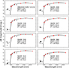 |
Fig. C.1. SED fits for all 16 targets. We show the best-fit Castelli & Kurucz model (in black) and associated stellar and extinction parameters. The red points denote photometry given weight in the fit. The black points are shown for comparison. |
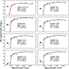 |
Fig. C.1. Continued. |
Appendix D: Spectral type variability
Table D.1 displays the various spectral classifications for the star SkKM 250.
RMC 29 spectral type variability.
Appendix E: Discussion of individual targets
In this section we highlight two of the targets that have notable properties. Firstly, we assess the status of SkKM 250 as a member of the SMC and we then discuss the significance of the high effective temperature of SkKM 247.
E.1. SkKM 250
The 3σ significant Gaia parallax of SkKM 250 implies a geometric distance of 12 kpc (Bailer-Jones et al. 2021). The kinematic properties of this source all appear consistent with SMC membership and various luminosity classifications place this star in the SMC. However, if the metallicity of the star is significantly lower than assumed when determining the spectral type, the luminosity class is likely to be unreliable. In their analysis of SMC RSGs, based on the elemental abundance pattern compared to the rest of their sample, Hill (1997) considered whether this star is a galactic halo star. Hill concluded that this star is a member of the SMC. Using the neural network classifier of Jiménez-Arranz et al. (2023) the likelihood of SMC membership for SkKM 250, based on its Gaia DR3 measurements is 51 %, which would mean that this source would be included in both their ‘complete’ and ‘optimal’ samples.
If we assume that the distance provided by Bailer-Jones et al. (2021) is correct this implies that SkKM 250 is giant star in the halo of the Milky Way. The luminosity of the hot companion in this scenario would be logL/L⊙ = 2.52 ± 0.40, assuming the 16th to 84th percentile confidence interval on the Bailer-Jones et al. (2021) distance to determine the uncertainties. This would make the hot companion a subdwarf OB-type star. Typically sub-dwarf B stars have luminosities up to logL/L⊙ ∼ 1.5 (Moehler et al. 1997) and logL/L⊙ = 2.52 ± 0.40 is potentially larger than theoretically possible for such stars (Han et al. 2002). Therefore, we prefer the explanation that SkKM 250 is an SMC member, but acknowledge that the distance uncertainty makes the interpretation as a Galactic halo star a viable option. We assume the Gaia DR4 parallax will resolve this uncertainty, but if not, a full binary solution may be the best method for distinguishing between these scenarios. We retain this star in our sample and consider it an SMC member for the purposes of the discussion.
SkKM 250 is the only target that was observed to have an additional target within the slit. This secondary source is 1.7″ from the SkKM 250, which corresponds to a physical distance in the SMC of ∼0.5 pc. We identified the source as Gaia DR3 4690509117967865344, with a G-band magnitude of 17.2. We extracted the spectrum of the source and find it consistent with an early-type star. Given the physical separation of 0.5 pc, we consider it possible, but unlikely, that the sources are physically associated.
E.2. SkKM 247
The hot companion of SkKM 247 has one of the highest temperatures determined in the sample, which, for the luminosity of the star, places it far to the left of the main sequence. The effective temperature range for this star is 30–40 kK, with a radius that appears smaller than that of the other sources. To make this source consistent with the main-sequence position of the models requires a temperature at the lowest end of this range, this in turn implies very small, if not negligible, reddening values. In contrast, the SED fitting this source has among the largest determined E(B − V) = 0.11, which is still relatively modest. In addition, as noted in Appendix B, this source shows a Ks − [24μm] excess that suggests a reddening value of E(B − V) = 0.096, in good agreement with the SED fitting. This is marginally larger, but fully consistent with the value determined from the comparison with nearby O-type stars (i.e. E(B − V) = 0.076). Assuming E(B − V) = 0.11 from the SED fitting, places the effective temperature around 40 kK, clearly to the left of the main sequence given its luminosity. The Swiftuvm2 absolute magnitude of this source is comparable with a ∼5 M⊙ B-type SMC stripped star (Drout et al. 2023), which would imply an effective temperature of at least 60 kK, which is inconsistent with the temperature estimates from the near-UV spectra. In addition, at this mass we might expect to observe He II absorption features (Götberg et al. 2018), which are absent from the spectrum (see Fig. A.5).
At present we consider this source as broadly consistent with being on the main sequence but consider this source the best candidate so far for a stripped star companion to a RSG. This will be assessed in greater detail in a third paper in this series using shorter wavelength HST spectra.
All Tables
Spectral types, IDs, and stellar parameters of the RSG components of the systems.
Stellar parameters for the hot companions to RSGs as determined by the HST/STIS Snapshot spectra.
All Figures
|
Fig. 1. Montage of the observed HST/STIS UV spectra. Each spectrum has a S/N per resolution element of at least 30 at ∼2400 Å, ranging to ∼60 for LHA 115-S 7. The flux distribution is not normalised, to enable a better visualisation of the hot star continuum. Line identifications are marked in grey; however, we note that the only features detectable in the spectra are of interstellar origin and not suitable for stellar parameter determination. No normalisation factor is applied to any of the spectra displayed here. All 16 spectra are shown individually in Appendix A. |
| In the text | |
|
Fig. 2. Left: HRD for the 16 targets with stellar parameters determined from the G230LB STIS spectra, shown as blue stars. The blue point shows the typical uncertainties on the stellar parameters (see Section 3.1 for more details and caveats). The grey lines show SMC stellar tracks using a mass-dependent overshooting parameter (Schootemeijer et al. 2019; Hastings et al. 2021), where dashes are marked at intervals of 0.05 Myr. The dashed lines show isochrones of ages 10, 20, and 30 Myr. Spectral types for SMC dwarf stars are shown using the calibration presented in Shenar et al. (2024). Large black circles mark the stars labelled ‘embedded’ in Table 3. Right: Same as the left panel but we add the stellar parameters determined from Patrick et al. (2022) in red. The uncertainties are illustrated with the red point. Black lines connect the stellar parameters derived using the two methods. |
| In the text | |
|
Fig. 3. Example of the SED fitting to determine the stellar parameters of the RSG component. The large red points are from Gaia and 2MASS and are the only photometry given weight in the fit. Black points are from Skymapper, Swift, and UVIT. |
| In the text | |
|
Fig. 4. Comparison of the ages of the hot companions (abscissa) and the RSG components (ordinate) of the 16 binary systems studied. The dashed grey line shows the expectation of coevality, i.e. a one-to-one relationship. The ages of the two components are inconsistent in seven of the 16 cases at the ∼3σ level. These sources are marked with red stars. The black point on the left indicates the typical uncertainties. |
| In the text | |
|
Fig. 5. Two examples of HST/STIS G230L spectra that deviate from a normal B-type star continuum. This behaviour is observed in SkKM 108, 209, 286, and 320 (209 and 286 shown in this figure). The red spectrum shows an IUE spectrum of 32 Cyg published in Che et al. (1983) at an orbital phase of 0.7. The blue spectrum shows an example of a normal B-type spectrum of Alpha Sco B from unpublished IUE data retrieved from the INES database (programme ID LGLMS; PI: M. A. Smith), which highlights the differences observed. Note that as the comparison stars (Alpha Sco B and 32 Cyg) are both galactic stars, the flux distribution bluewards of ∼2500 Å is different as a result of the differing extinction laws in the two galaxies. Line identifications are shown in grey. We note that in the SMC spectra the Mg II feature is dominated by the interstellar component. |
| In the text | |
|
Fig. A.1. Example of the result of the χ-squared fitting procedure for SkKM 113. The black line shows the observed data, and the red line the best-fitting model with an effective temperature of 25kK and logg = 4.0. The red star marks the synthetic photometry in the UVIT F172M band, which was computed directly from the HST spectrum. The green star marks the UVIT F172M magnitude from Thilker et al. (in prep.). The difference in magnitude between the two is ∼0.3mag. |
| In the text | |
|
Fig. A.2. HST/STIS spectrum of SkKM 320. |
| In the text | |
|
Fig. A.3. HST/STIS spectrum of SkKM 286. |
| In the text | |
|
Fig. A.4. HST/STIS spectrum of SkKM 90. |
| In the text | |
|
Fig. A.5. HST/STIS spectrum of SkKM 247. |
| In the text | |
|
Fig. A.6. HST/STIS spectrum of LHA-115-S-7. |
| In the text | |
|
Fig. A.7. HST/STIS spectrum of M2002-SMC-54134. |
| In the text | |
|
Fig. A.8. HST/STIS spectrum of SkKM 209. |
| In the text | |
|
Fig. A.9. HST/STIS spectrum of SkKM 310. |
| In the text | |
|
Fig. A.10. HST/STIS spectrum of SkKM 74. |
| In the text | |
|
Fig. A.11. HST/STIS spectrum of SkKM 113. |
| In the text | |
|
Fig. A.12. HST/STIS spectrum of PMMR-61. |
| In the text | |
|
Fig. A.13. HST/STIS spectrum of SkKM 171. |
| In the text | |
|
Fig. A.14. HST/STIS spectrum of SKKM 250. |
| In the text | |
|
Fig. A.15. HST/STIS spectrum of SKKM 108. |
| In the text | |
|
Fig. A.16. HST/STIS spectrum of SKKM 238. |
| In the text | |
|
Fig. A.17. HST/STIS spectrum of SKKM 239. |
| In the text | |
|
Fig. B.1. Ks-band magnitudes (MKs) vs Ks − 24μm colour-magnitude diagram for SMC RSGs (grey points) from Patrick et al. (in prep.). The red diamonds show RSGs observed with UV SITS spectroscopy. |
| In the text | |
|
Fig. C.1. SED fits for all 16 targets. We show the best-fit Castelli & Kurucz model (in black) and associated stellar and extinction parameters. The red points denote photometry given weight in the fit. The black points are shown for comparison. |
| In the text | |
|
Fig. C.1. Continued. |
| In the text | |
Current usage metrics show cumulative count of Article Views (full-text article views including HTML views, PDF and ePub downloads, according to the available data) and Abstracts Views on Vision4Press platform.
Data correspond to usage on the plateform after 2015. The current usage metrics is available 48-96 hours after online publication and is updated daily on week days.
Initial download of the metrics may take a while.