| Issue |
A&A
Volume 700, August 2025
|
|
|---|---|---|
| Article Number | A55 | |
| Number of page(s) | 8 | |
| Section | The Sun and the Heliosphere | |
| DOI | https://doi.org/10.1051/0004-6361/202554165 | |
| Published online | 05 August 2025 | |
Detecting in situ directional discontinuities in the Solar Wind at Mercury’s orbit
1
INAF-Institute for Astrophysics and Space Planetology, Via del Fosso del Cavaliere, 00133 Roma, Italy
2
Department of Physics, University of Rome Tor-Vergata, Via della Ricerca Scientifica, 00133 Rome, Italy
3
Istituto Nazionale di Geofisica e Vulcanologia, Rome, Italy
4
Space Research Institute, Austrian Academy of Sciences, Graz, Austria
5
Institut für Geophysik und Extraterrestrische Physik, Technische Universität, Braunschweig, Germany
6
Max Planck Institute for Solar System Research, Justus-von-Liebig-Weg 3, 37077 Göttingen, Germany
7
Italian Space Agency, Rome, Italy
⋆ Corresponding author: This email address is being protected from spambots. You need JavaScript enabled to view it.
Received:
17
February
2025
Accepted:
13
June
2025
Abstract
Context. Since at closer distances to the Sun the solar wind is highly structured, the analysis of directional discontinuities (DDs) provides further insights into the physical properties of its embedded structures.
Aims. By combining magnetic field and PICAM ion sensor observations, we investigated the occurrence rate and nature of DDs observed by BepiColombo close to Mercury’s orbit.
Methods. We used the magnetic field attitude gradient method to detect discontinuities combined with minimum variance analysis to classify the boundaries of the structures.
Results. During the selected period between 5 and 16 October 2021, 960 DDs were identified. The majority (83%) were rotational discontinuities (RDs) or either discontinuities (EDs). Low compressibility (CB < 0.03) conditions yielded a higher fraction of RDs and EDs (94%). PICAM observations revealed ion energy enhancements and particle deflections correlated with magnetic field reversals, particularly during structures characterised by low compressibility.
Conclusions. The results suggest that between 5 and 16 October 2021, BepiColombo observed a series of DDs compatible with the boundaries of magnetic switchbacks, characterised by low compressibility, which is expected for Alfvénic structures. The increase in energy and ion differential energy flux, despite the unfavourable aberration angle, and ion flux spikes strongly correlated with magnetic field reversals, could be explained by field-aligned particles that do not reverse their pitch angle.
Key words: plasmas / Sun: magnetic fields / solar wind
© The Authors 2025
 Open Access article, published by EDP Sciences, under the terms of the Creative Commons Attribution License (https://creativecommons.org/licenses/by/4.0), which permits unrestricted use, distribution, and reproduction in any medium, provided the original work is properly cited.
This article is published in open access under the Subscribe to Open model. This email address is being protected from spambots. You need JavaScript enabled to view it. to support open access publication.
1. Introduction
Since the early 1960s, extensive research has focused on understanding and characterising the evolution of solar wind properties and structures (Bruno & Carbone 2016). The continuous and currently growing interest is driven by their relevance to key questions in space physics. This includes, among others, their possible role in solar wind acceleration and/or heating mechanisms, and in affecting nonlinear interactions among eddies and the turbulent energy cascade, their interaction with planetary environments, and the occurrence of solar-origin transient events (Tu & Marsch 1995; Burlaga 2001; Horbury & Balogh 2001; Verscharen et al. 2019). As these structures interact with the ambient solar wind, they can experience acceleration or deceleration, forming compression regions and triggering in situ phenomena such as shocks and particle acceleration (Bale et al. 2005). Usually, structures are identified by their signature in the magnetic field components, typically associated with rotations of one or more components. As an example, magnetic flux ropes can be identified through their helical field lines winding around a common strong axial-aligned core (Zheng & Hu 2018; Hu et al. 2018). They may both originate from the magnetic reconnection at the solar corona (Sanchez-Diaz et al. 2017) or due to in situ developments in quasi-2D turbulence (Greco et al. 2009; Wan et al. 2013). They have been frequently observed throughout the heliosphere at different heliocentric distances, between 0.3 and 5.5 (Cartwright & Moldwin 2010).
There has also been recent interest in S-shaped kinks in the interplanetary magnetic field (IMF), which result in a sharp polarity inversion at their crossings (Bale et al. 2019; Kasper et al. 2019; Dudok de Wit et al. 2020; Horbury et al. 2020), both close to the Sun and far away, known as magnetic switchbacks (SBs). While their presence has been observed since the 1980s at large heliocentric distances (Behannon & Burlaga 1981; Kahler et al. 1996; Van Ballegooijen et al. 1998; Balogh et al. 1999; Yamauchi et al. 2004; Landi et al. 2006; Neugebauer 2012; Neugebauer & Goldstein 2013; Matteini et al. 2014; Borovsky 2016; Horbury et al. 2018), more recently Parker Solar Probe (PSP) revealed that closer to the Sun the solar wind is highly structured and SBs are frequently observed (Bale et al. 2019; Kasper et al. 2019; Dudok de Wit et al. 2020; Horbury et al. 2020; Larosa et al. 2021). Switchbacks are usually observed in Alfvénic streams, with a nearly constant magnetic field amplitude and displaying a high correlation between magnetic and velocity fields (Agapitov et al. 2023), although some SBs are characterised by a compressible nature (Larosa et al. 2021). Their origin remains highly debated, with two main theories attributing their formation either to interchange reconnection below the Sun’s source surface (Fisk & Kasper 2020; Zank et al. 2020) or to processes occurring during solar wind propagation, such as Alfvén wave turbulence (Squire et al. 2020; Shoda et al. 2021; Mallet et al. 2021), Kelvin-Helmholtz instability or shear-driven turbulence (Ruffolo et al. 2020).
An important step towards understanding solar wind structures involves investigating their boundaries. These boundaries often appear as directional discontinuities (DDs), defined by abrupt changes or rotations in the magnetic field over short time intervals (Burlaga 1968; Mariani et al. 1973; Tsurutani et al. 1995; Tsurutani & Ho 1999). Directional discontinuities are thought to play a key role in several fundamental processes, including particle acceleration, energy dissipation, and wave–particle interactions. A characteristic feature of these structures is the presence of narrow current layers embedded within the discontinuity, which have been revealed by recent observations (Artemyev et al. 2018; Krasnoselskikh et al. 2020). In particular, a statistical study by Larosa et al. (2021) focusing on the boundaries of SBs at heliocentric distances of 0.18–0.2 AU found that the associated currents can be up to two orders of magnitude stronger than the ones typically measured at 1 AU. Different types of DDs have been identified based on their rotational properties and magnetic field intensity gradients (Smith 1973). Rotational discontinuities (RDs) are essentially short-wavelength Alfvén waves that have mass flow across their surface (Tsurutani et al. 1994; Tsurutani & Ho 1999). They are characterised by a large field normal component and no changes in the magnetic field magnitude. These features make them compatible with the edges of SBs trains, where they are often observed. They move at the Alfvén speed with respect to the plasma, and they may be involved in scattering charged particles as they propagate from one region to another. On the other hand, tangential discontinuities (TDs) have no mass flux across their surface, then they separate two different sides of plasma regions, i.e. with different magnetic field directions and magnitudes, plasma densities, temperatures, and compositions. They are identified by a small field normal component and a large jump in the magnetic field magnitude between the two sides of the discontinuity and they propagate with the solarwind speed.
In this paper, we use BepiColombo (BC; Benkhoff et al. 2021) observations just after its first flyby of Mercury in October 2021. In particular, we use the MPO-MAG magnetic field measurements and the solar wind observations by the Planetary Ion CAMera (PICAM). With magnetic field measurements, we identify and classify the DDs following the minimum variance analysis (MVA) technique. By combining PICAM and MAG observations, we discuss the possible detection of SBs close to Mercury’s orbit. The paper is organised as follows. Section 2 presents the discontinuities selection and classification algorithms. In the same section, key parameters, such as magnetic compressibility and normalised deflection, are defined to characterise the observed structures. Section 3 provides an overview of the data and instruments. Section 4 presents and discusses the statistical analysis carried out on the DDs using the magnetic field measurements. When available, plasma measurements complement the study of the solar wind structures. with boundaries associated with the detected DDs.
2. Methods
Several methods aimed at establishing quantitative criteria for the automatic detection of DDs have been introduced since the beginning of solar wind exploration (Tsurutani & Smith 1979; Vasquez et al. 2007; Erdos et al. 2001). In our analysis, we used the method introduced by Erdos et al. (2001) and described in detail by Erdos & Balogh (2008). All the studies mentioned are based on Ulysses data, but the same method was used to analyse the radial decaying of magnetic field DDs also in the vicinity of the Sun by means of PSP and Solar Orbiter (SolO) observations (Madar et al. 2024). The first step of the algorithm was to evaluate the gradient of the magnetic field unit vector as a function of time. To discard small-scale irregularities of magnetic field data, we used a moving average over a Δt = 10 s sliding window to exploit the full time resolution of the data, and we evaluated the angle
 (1)
(1)
Then, the attitude gradient was defined as
 (2)
(2)
The magnetic field DDs were identified by finding the local maxima of the attitude gradient, amax, that exceeded a fixed threshold, ac, and then by checking that the nearest local minima (at the time, tu, before and td, after) were lower than amax/2. This condition must be satisfied not only by local minima, but also in the two time windows, upstream, Iu = [tu − l, tu], and downstream, Id = [td, td + l], of length l = td − tu, i.e.
 (3)
(3)
In contrast to other authors (Erdos & Balogh 2008; Madar et al. 2024), we considered the dependence on time in the attitude gradient, instead of using Taylor’s hypothesis to translate it into velocity. This was because we could not access the velocity data for the period under consideration. In Figure 4 panel b an example of the parameter, ac, computed for 6 October 2021 is shown.
After deriving the timing of DDs, we needed to characterise their geometry and nature in order to provide a statistical classification (Smith 1973; Neugebauer et al. 1984). For this purpose, we used the MVA (Sonnerup 1998), which allowed us to detect the normal direction to the DD surface. The detected DDs were classified according to the discontinuity parameters reported in Table 1.
DD classification.
The term Bmax indicates the IMF magnitude peak in the DD interval [tu, td] for the normal parameter and in the upstream, Iu, and downstream, Id, intervals for the tangential one,  , where
  is the DD normal vector, and Δ|B| is the difference between the quiet upstream and downstream mean values of the IMF magnitude. We note that the MVA technique could be inaccurate (Horbury et al. 2001; Knetter et al. 2004), producing normal angles that deviate more than 60° with respect to theeffective normal directions, even when the ratio between medium and minimum eigenvalues is relatively high (e.g. λmed/λmin ≈ 4) (Wang et al. 2024). However, this method remains a valuable tool for investigating the nature of the discontinuities with single-point measurements. It provides reasonable estimates in our analysis, yielding consistent results for the occurrence rate of DD types when considering a ratio between the medium and minimum eigenvalue, λmed/λmin > 2, as well as for a threshold of 4 (not shown). Since it is possible that the chosen window could not be the optimal one, we shortened or lengthened it by 25%. However, the number of detected discontinuities is quite stable (1022 vs. 943) within the ±25% range of uncertainty. Since SBs are usually observed in Alfvénic streams (Larosa et al. 2021), we also evaluated the magnetic compressibility as a proxy for the Alfvénicity of the observed solar wind, by measuring the ratio
 (4)
(4)
where σ⋅ denotes the standard deviation of the vector field ⋅ and i ∈ {R, T, N}. CB weights the variance of the IMF magnitude, B, with respect to its trace (Tu & Marsch 1995; Bruno & Carbone 2013) We relied on CB as a measure of compressibility due to the lack of measurements of solar wind plasma parameters, which prevented us from properly estimating correlations between magnetic and velocity field fluctuations.
To classify specific types of DDs as SBs, we evaluated the normalised deflection parameter, z, which quantifies the rotation of the local IMF with respect to a background mean field, defined as Dudok de Wit et al. (2020)
 (5)
(5)
where α is the angle between the local IMF and the mean field ⟨B⟩ averaged over 6 h. The value of z ranges between 0 and 1, where z = 0 (z = 1) indicates that the magnetic field is parallel (antiparallel) to the mean field. In this work, we consider, as a suitable threshold to constrain SBs, magnetic deflections larger than 90°, i.e. z > 0.5, according to Pecora et al. (2022).
3. Data
We focused on the period between 5 and 16 October 2021, when BC was located at a heliocentric distance ranging between 0.32 and 0.35 AU. This allowed us to explore the ambient solar wind properties close to Mercury’s orbit, which are less affected by its radial evolution if a longer period is considered. We used magnetic field measurements collected by the 3D fluxgate magnetometer MPO-MAG (Heyner et al. 2021; Glassmeier et al. 2010) with a time resolution of 1 s in the radial-tangential-normal (RTN) coordinate system. MPO/MAG consists of two identical fluxgates mounted on a boom deployed soon after launch. Since then, the IMF has been measured almost continuously at a distance of 2.9 m from the spacecraft and the instrument has been calibrated regularly. Figure 1 reports the magnetic field data in the RTN reference frame (panels a, b, c, d) together with the magnetic compressibility, CB, and the normalised deflection parameter, z, both computed over the whole period.
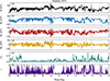 |
Fig. 1. Magnetic field magnitude (a), components in the RTN reference frame (b)–(d), magnetic compressibility (e), and the deflection parameter (f) during the interval of interest between 5 to 16 October 2021. |
The ion data during the interplanetary cruise of BC were collected by PICAM, the ion mass spectrometer of the Search for Exospheric Refilling and Emitted Natural Abundances (SERENA) (Orsini 2021). The solar wind sensor has an energy range from a few electronvolts to ∼3 keV, a mass range extending up to approximately 132 amu, and an instantaneous field of view (FoV) of approximately 1.5 π (Orsini 2021). In the selected periods, it was operated in solar wind mode, i.e. without mass resolution and in the energy range of 500–3000 eV. During the BC cruise phase, the PICAM boresight, d, is oriented in a direction perpendicular to the spacecraft-Sun line. Therefore, the solar wind can only partially enter the detector, depending on the aberration due to the spacecraft velocity, VSC. The optimal configuration for measuring solar wind ions is when the angle, γ, between the velocity and the instrument boresight is small. Furthermore, during the BC cruise, PICAM measurements are not continuous but are only available during some selected time windows. Figure 2 shows the PICAM spectrograms (panel a) provided as differential energy flux in the available time windows between 6 and 8 October 2021, the magnitude and radial component of the magnetic field (panel b), the magnetic compressibility, CB (panel c), and the deflection parameter, z (panel d).
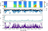 |
Fig. 2. Overview of the particle spectrograms and magnetic field time series observed by BC between 6 and 8 October 2021. (a) Ion energy spectrograms by PICAM in units of differential energy flux (dE flux) [cm−2 s−1 sr−1 eV/eV]; (b) radial magnetic field component (blue) and magnetic field magnitude (black); (c) magnetic compressibility, CB; (d) deflection parameter, z. |
4. Results
4.1. Statistical analysis of directional discontinuities
As a first step in our analysis, we need to select an appropriate threshold, ac, of the attitude gradient based on the statistics of the number of DDs identified as a function of ac. Figure 3 reports the number of DDs identified from MPO-MAG data for different ac values.
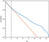 |
Fig. 3. Number of DDs identified on the BC data sample as a function of the threshold ac on the attitude gradient. The red line indicates the exponential trend fitted at small ac, and the vertical line marks the value of ac used in the present study. |
We set as a threshold the value of the attitude gradient at which the trend of the number of DDs departs from an exponential decay (red line in Figure 3), corresponding to ac = 2° /s, while, for larger values of ac, NDD continues to decrease at a slower rate. This threshold in the DD detection algorithm is consistent with other studies on different spacecraft data and at different heliocentric distances (e.g., Madar et al. 2024). The total number of DDs identified by the attitude gradient method with ac = 2° /s from BC observations is 1136. Figure 4 shows an example of DD identification using the gradient method with the same threshold, based on magnetic field measurements on 6 October 2021.
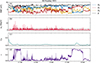 |
Fig. 4. Time series of the IMF and derived parameters on the day of 6 October 2021 between 09:30 and 20:00 UT. Panel (a): radial (BR, blue), tangential (BT, red), normal (BN, yellow) components, and intensity (B, black) of the magnetic field. Panel (b): attitude gradient, ag, with the chosen threshold at 2° s−1, represented by the horizontal dashed black line. Panel (c): magnetic compressibility, CB, where the horizontal dashed black line represents the threshold set at 0.03. Panel (d): normalised deflection parameter, z. |
Rapid magnetic field rotations and reversals (Figure 4(a)) of different durations closely correspond to peaks in the attitude gradient, ag(t) (Figure 4(b)). Between 10:30 and 11:30 and between 17:00 and 19:00, two distinct slow-reversing structures are observed. Notably, in these structures z ∼ 1 for a longer time, corresponding to a net decrease in compressibility CB, indicating a more Alfvénic solar wind. Furthermore, several shorter-duration reversals (with timescales from seconds to minutes) are highlighted by the attitude gradient, characterised by many high peaks above the threshold. We discuss these events in more detail in Section 4.2, in light of the particle measurements provided by PICAM. To investigate the occurrence and the nature of DDs observed by BC, we thereforeperformed the Neugebauer et al. (1984) classification, allowing us to make a direct comparison between statistical results recently obtained in the inner heliosphere with other probes (Madar et al. 2024). Figure 5 shows the scatter plot of the change in the IMF magnitude, |ΔB|, across the discontinuity, identified through the maxima of the attitude gradient, a(t), versus the absolute value of the normal magnetic field component, Bn, detected through MVA, both normalised for the maximum field value, Bmax, as is described in Section 2.
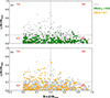 |
Fig. 5. DD classification according to Neugebauer et al. (1984). The dotted lines separate the different discontinuity areas, while grey symbols identify different types (triangles, TD; circles, ED; squares, ND; and stars, RD). Green symbols in panel (a) represent the subset of DDs satisfying the low-compressibility condition (CB < 0.03), while orange symbols in panel (b) refer to z > 0.5. |
The grey symbols in panels (a) and (b) of Figure 5 report the DD parameters that satisfy the MVA condition with a ratio between the medium and minimum eigenvalue greater than 2, detecting a total number of 960 discontinuities. The green and orange symbols refer to low-compressibility conditions (CB < 0.03) and high deflection angles (z > 0.5), respectively, which may indicate the presence of SBs. Our results align with previous findings observed at larger heliocentric distances (e.g., Table 2 in Neugebauer et al. 1984; Neugebauer 2006) and (Figure 9 in Söding et al. 2001). DDs with a high variation of B (i.e., TD and ND) represent the minority part of the statistics, which is thus dominated by EDs and RDs. Specifically, we found that 45% of the DDs are EDs, 38% are RDs, 11% are TDs, and 6% are NDs. Moreover, by conditioning our sample to a low compressibility, CB < 0.03, where the chosen threshold corresponds approximately to the 25-th percentile, the percentage of ED and RD increases with respect to the unconditioned values up to 49% and 41%, while TDs and NDs decrease to 7% and 3% (Figure 5(a)). This result is consistent with previous findings on the analysis of SBs’ leading and trailing edges, mainly based on PSP observations (see, e.g., Akhavan-Tafti et al. 2021; Larosa et al. 2021).
On the contrary, by conditioning instead on the z parameter for z > 0.5 (Figure 5(b)), the number of discontinuities decreases drastically to 169 with 47% being EDs, 27% RDs, 21% TDs, and the remaining 5% NDs. Although there is a low sample of statistics, the majority of DDs with a large deflection, i.e. larger than 90°, are of the ED type, while the numbers of RDs and TDs are fairly balanced. In this case, the conditioning does not result in meaningful differences in the DD-typestatistics.
Then, we further introduced conditioning with respect to a time division based on the compressibility trend. We divided the whole period into the interval, IC, which extends from 09:45 UT on 6 October to 15:30 UT on 12 October and is characterised by rather low values of magnetic compressibility (as is shown in panel d of Figure 1), and the second is given by the union of the intervals to the left and right of IC. We found that in IC there are a total of 628 DDs, with 49% EDs, 41% RDs, 6% TDs and 4% NDs, while in IR we have 332 DDs, with 38% EDs, 33% RDs, 19% TDs, and 10% NDs, confirming that the period of low compressibility presents a net prevalence of the ED and RD types. Finally, the statistics on IC|CB < 0.03 show that the majority of the discontinuities present on the whole set and conditioned on CB belong to IC (243 on 280), maintaining percentages almost unchanged. All these results are summarised in Table 2.
Summary of the statistics.
In the non-compressible interval, Ic, which exhibits a higher prevalence of ED and RD types than Ir, most DDs are compatible with the edges of the SBs (see Table 2). In fact, by conditioning to the parameter z (Fig. 5(b)) we note that, although it is a convenient proxy to identify relevant field deflections as SBs, the statistics of the DD types are not affected by its value. By contrast, magnetic compressibility, CB, is an effective proxy for identifying ED and RD types, and consequently for determining structure boundaries exhibiting these features.
4.2. PICAM observations and SBs
The limited FoV by PICAM can instead be used to probe solar wind structures that may be identified as SBs. Indeed, the possibility of joining the DD analysis of the magnetic field with the ion measurements provided by PICAM enables a more robust physical interpretation of some of the statistical results presented in the previous section about Alfvénic structures. Figure 6 shows four time intervals characterised by magnetic field reversals in correspondence of PICAM observing time windows.
During the first PICAM observation on the day of 6 October 2021 between 08:37 and 13:28 UT, shown in Figure 6(a1), it is possible to observe the occurrence of a plasma structure between 10:00 and 11:00 UT. Initially (before 10:00 UT), the ion flux measured by the sensor reveals an ambient slow solar wind stream with energy of about 600–700 eV. However, between 10:00 and 11:00 UT higher-energy particles up to 1 keV are detected. Simultaneously, all the magnetic field components rotate, suggesting the presence of a large-scale structure, and a strong deflection from the mean magnetic field (z ≈ 1), reported, respectively, in panels (c1) and (e1) of Figure 6. It is important to note that the variation in flux intensity observed by PICAM is affected by three main factors: (1) the variability of the ambient solar wind, (2) the spin of the spacecraft, rotating towards more or less favourable conditions for the PICAM FoV to sample different parts of the solar wind particle distribution function, and (3) the magnetic field rotations driving the suprathermal plasma distribution towards or away from the FoV. Factors (1) and (3) are physical, while factor (2) is an effect due to the spacecraft’s motion. Anyway, since the spacecraft rotation is much slower than the ambient solar wind variations, we are able to discriminate factor (2) from factors (1) and (3). Since the energy behaviour is not related to the spacecraft’s rotation (see Figure 6(b1)), while it is clearly related to the radial component of IMF (see Figure 6(c1)), then the observed increase can be attributed to the sampling of a solar wind structure, characterised by lower compressibility (see Figure 6(d1)) and higher values of the parameter z (see Figure 6(e1)).
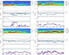 |
Fig. 6. Four selected time intervals during PICAM observation time windows. For each observation, panels (a) report the ion energy spectrograms by PICAM and the inverse of the IMF radial component, −BR, panels (b) the cosine of the scalar product between the PICAM boresight and the spacecraft velocity, CVSC, (c) the radial component (blue) and magnitude (black) of the magnetic field, (d) the magnetic compressibility, CB, and (e) the normalised deflection parameter, z. |
We remark that during the first part of the observation the instrument pointing was favourable for the aberration until 10:35 UT. In fact, the parameter CVSC, shown in panel b1 of Figure 6, increases up to values close to 1, indicating that, with the spacecraft’s rotation, the boresight becomes almost aligned with the spacecraft velocity direction, allowing the optimal FoV configuration corresponding to the highest values of the observed fluxes. Then, because of the spacecraft’s rotation, the data gradually show that only a small part of the solar wind particles’ distribution could enter within the PICAM FoV. Indeed, the boresight direction moves away from the optimal configuration until the rotation stops and remains stable at values close to 0 (see Figure 6(b1)), leading to a reduced portion of solar wind entering into the FoV and the lowest fluxes in the second part of the instrument observation. The slight energy increase is observed when the pointing moves to a favourable configuration. Moreover, a clear decrease in magnetic compressibility occurs at 09:40 UT, coinciding with the crossing of the structure. It remains stable at low values, with a mean value of 0.058, in the following days until 12 October at 15:30 UT. The physical features, highlighted by plasma and magnetic data, which include a fairly stable field magnitude, jointly with the trend of the derived parameters, suggest that the identified structure on 6 October between 10 and 11 UT could be a large-scale SB. Furthermore, as can be seen in Figures 4(a),(d), a similar event, marked by a complete rotation of the field components and an important deflection from the ambient magnetic field of about 180°, is detected on the same day between 17:30 and 19:05, but, unfortunately, not supported by the PICAM measurements.
This set of PICAM observations (see Figure 2(a)), characterised, as was mentioned above, by rather low values of compressibility, (see Figure 4(c)) and therefore with a possible Alfvénic nature of the stream explored, collects events with characteristics compatible with SBs. In fact, by zooming in on smaller-scale structures, we observe that in association with large sudden IMF deflections (z ≥ 0.5) particles suddenly enter the partial FoV of the instrument. This is clearly seen at 12:00 and 12:30 UT on 6 October (Figure 6 panel a1) and at 17:35 UT on 7 October (Figure 6 panel a3), just during periods when the PICAM instrument is not in a favourable orientation to measure the solar wind stream (CVSC ≃ 0.2 in panel b1, and CVSC ≃ −0.2 in panel b3 of Figure 6). In contrast, the observation during the time window of 8 October exhibits a continuous profile in the energy signal with a higher flux intensity, as is shown in panel a4 of Figure 6, due to a stable and optimal FoV configuration (CVSC ≃ 1 in panel b4 of Figure 6). Moreover, if the increased particle counting is associated with an increase in particle density, the energy bins over which the increase occurs provide an estimation of the change in particle velocity. By inspecting the IMF radial component and the deflection parameter, as was mentioned above, we find evidence of a strong correlation between the occurrence of fast IMF polarity inversions and the energy profile of particles observed by PICAM, as is shown in the panels a, c and e of Figure 6. Notably, the fluctuations of the magnetic field radial component correlate very well to the profile of the PICAM ion energy (Figure 6, panels a). The physical origin of these observations could be ascribed to field-aligned ion population entering the FoV of the instrument due to the IMF polarity reversals, despite the unfavourableobservation angle.
The increase in plasma fluxes and energy (i.e. velocity) when the magnetic field rotates gives even more evidence of their correlation. This is consistent with the scenario that emerged from the DDs analysis. In fact, the large presence of ED and RD type radial reversals in the interval, statistically associated with low compressibility, confirms the correlation between the velocity and magnetic field fluctuations highlighted by PICAM.
5. Conclusions
The identification and characterisation of structures in the solar wind is a long-standing problem intimately related to the investigation of their boundary layers using in situ spacecraft measurements. In this paper, we have analysed BC data to add another piece of knowledge to the puzzle of inner heliospheric observations by exploring magnetic DDs in the near-Mercury environment at a radial distance of 0.33–0.36 AU. Our results are in line with previous observations based on PSP and SolO (Madar et al. 2024), but also with findings in the outer heliosphere based on Ulysses data (Tsurutani et al. 1996; Tsurutani & Ho 1999). The unavailability of continuous plasma measurements and the restricted FoV of instruments on board BC during this part of the cruise make the investigation of solar wind structures challenging. However, we show that the IMF diagnostics, such as the CB parameter, allow for a reasonable exploration of the nature of the observed structures. We characterise the Alfvénic structures through a DD analysis from the largest scales to the smaller ones. The Smith classification of DDs reveals the predominance of boundary layers with small |ΔB| such as ED and RD types. EDs are typically associated with current sheets, having a reduced normal component, whereas RDs are mainly related to Alfvénic jumps. This fact is supported by the DD analysis conditioned on magnetic compressibility, which leads to an even stronger predominance of low |ΔB| DDs. TDs, on the other hand, are usually associated with current sheets.
The PICAM ion sensor operated during several observation windows in October 2021. The limited FoV of the ion sensor did not prevent it from highlighting the plasma behaviour during small-scale magnetic SBs. The absence of background solar wind due to a non-favourable spacecraft configuration, on the contrary, accentuated the time interval when SBs light up, by suddenly recording an increased particle counting with an energy profile that resembles the one of the magnetic field radial component, showing the strong Alfvénic nature of the observed fluctuations. This scenario opens new perspectives for future studies, highlighting that BC, thanks to its strategic position during the cruise and in the nominal phase, could play an important role not only in the heliosphere but especially near the Hermean environment. The impact of the structures on the Mercury’s magnetosphere could raise different phenomena (e.g. excitation of ultra-low-frequency, Kelvin-Helmholtz instabilities), which in turn could generate magnetic reconnection phenomena and substorm-like activity in the magnetotail, not yet observed by BC during the flybys performed in recent years.
Acknowledgments
This work was supported by the Italian Space Agency (ASI) and by the Italian National Institute of Astrophysics (INAF): SERENA agreement no. 024-66-HH.0 “Attività scientifiche per il Payload SERENA su BepiColombo, relative alla fine della fase di crociera e fase operativ”. PICAM is funded by the Austrian Space Applications Programme (ASAP) of the Austrian Research Promotion Agency (FFG), and partially by the Programme de Dévelopement d’Expériences (PRODEX), and by the CNES French Space Agency. MS acknowledges the financial support of the grant “Investigating the Universal Nature of Magnetic field Fluctuations in Solar Wind Turbulence” funded by the National Institute for Astrophysics under the call "Fundamental Research 2023. The SolO magnetometer was funded by the UK Space Agency (grant ST/T001062/1). D. Heyner was supported by the German Ministerium für Wirtschaft und Klimaschutz and the German Zentrum für Luft- und Raumfahrt under contract 50QW2202.
References
- Agapitov, O., Drake, J., Swisdak, M., Choi, K.-E., & Raouafi, N. 2023, ApJ, 959, L21 [Google Scholar]
- Akhavan-Tafti, M., Kasper, J., Huang, J., & Bale, S. 2021, A&A, 650, A4 [NASA ADS] [CrossRef] [EDP Sciences] [Google Scholar]
- Artemyev, A. V., Angelopoulos, V., Halekas, J. S., et al. 2018, ApJ, 859, 95 [Google Scholar]
- Bale, S., Kellogg, P., Mozer, F., Horbury, T., & Reme, H. 2005, Space Sci. Rev., 118, 161 [NASA ADS] [CrossRef] [Google Scholar]
- Bale, S., Badman, S., Bonnell, J., et al. 2019, Nature, 576, 237 [Google Scholar]
- Balogh, A., Forsyth, R., Lucek, E., Horbury, T., & Smith, E. 1999, Geophys. Res. Lett., 26, 631 [NASA ADS] [CrossRef] [Google Scholar]
- Behannon, K. W., & Burlaga, L. F. 1981, in Solar Wind Four, ed. H. Rosenbauer (Garching: Max-Planck-Institute für Aeronomie), 374 [Google Scholar]
- Benkhoff, J., Murakami, G., Baumjohann, W., et al. 2021, Space Sci. Rev., 217, 90 [NASA ADS] [CrossRef] [Google Scholar]
- Borovsky, J. E. 2016, J. Geophys. Res.: Space Phys., 121, 5055 [Google Scholar]
- Bruno, R., & Carbone, V. 2013, Liv. Rev. Sol. Phys., 10, 2 [Google Scholar]
- Bruno, R., & Carbone, V. 2016, Turbulence in the Solar Wind (Springer International Publishing Switzerland), 928 [Google Scholar]
- Burlaga, L. F. 1968, Sol. Phys., 4, 67 [Google Scholar]
- Burlaga, L. 2001, Planet. Space Sci., 49, 1619 [CrossRef] [Google Scholar]
- Cartwright, M., & Moldwin, M. 2010, J. Geophys. Res.: Space Phys., 115, A08102 [Google Scholar]
- Dudok de Wit, T., Krasnoselskikh, V. V., Bale, S. D., et al. 2020, ApJS, 246, 39 [Google Scholar]
- Erdos, G., & Balogh, A. 2008, Adv. Space Res., 41, 287 [NASA ADS] [CrossRef] [Google Scholar]
- Erdos, G., Balogh, A., & Kóta, J. 2001, Space Sci. Rev., 97, 221 [NASA ADS] [CrossRef] [Google Scholar]
- Fisk, L., & Kasper, J. 2020, ApJ, 894, L4 [Google Scholar]
- Glassmeier, K.-H., Auster, H.-U., Heyner, D., et al. 2010, Planet. Space Sci., 58, 287 [NASA ADS] [CrossRef] [Google Scholar]
- Greco, A., Matthaeus, W., Servidio, S., Chuychai, P., & Dmitruk, P. 2009, ApJ, 691, L111 [Google Scholar]
- Heyner, D., Auster, H. U., Fornaçon, K. H., et al. 2021, Space Sci. Rev., 217, 52 [CrossRef] [Google Scholar]
- Horbury, T., & Balogh, A. 2001, J. Geophys. Res.: Space Phys., 106, 15929 [Google Scholar]
- Horbury, T. S., Burgess, D., Fränz, M., & Owen, C. J. 2001, Geophys. Res. Lett., 28, 677 [Google Scholar]
- Horbury, T., Matteini, L., & Stansby, D. 2018, MNRAS, 478, 1980 [Google Scholar]
- Horbury, T. S., Woolley, T., Laker, R., et al. 2020, ApJS, 246, 45 [Google Scholar]
- Hu, Q., Zheng, J., Chen, Y., le Roux, J., & Zhao, L. 2018, ApJS, 239, 12 [Google Scholar]
- Kahler, S., Crocker, N., & Gosling, J. 1996, J. Geophys. Res.: Space Phys., 101, 24373 [Google Scholar]
- Kasper, J. C., Bale, S. D., Belcher, J. W., et al. 2019, Nature, 576, 228 [Google Scholar]
- Knetter, T., Neubauer, F. M., Horbury, T., & Balogh, A. 2004, J. Geophys. Res. Space Phys., 109, A06102 [Google Scholar]
- Krasnoselskikh, V., Larosa, A., Agapitov, O., et al. 2020, ApJ, 893, 93 [Google Scholar]
- Landi, S., Hellinger, P., & Velli, M. 2006, Geophys. Res. Lett., 33, L14101 [Google Scholar]
- Larosa, A., Krasnoselskikh, V., de Wit, T. D., et al. 2021, A&A, 650, A3 [NASA ADS] [CrossRef] [EDP Sciences] [Google Scholar]
- Madar, A., Opitz, A., Erdos, G., et al. 2024, A&A, 690, A328 [NASA ADS] [CrossRef] [EDP Sciences] [Google Scholar]
- Mallet, A., Squire, J., Chandran, B. D., Bowen, T., & Bale, S. D. 2021, ApJ, 918, 62 [NASA ADS] [CrossRef] [Google Scholar]
- Mariani, F., Bavassano, B., Villante, U., & Ness, N. F. 1973, J. Geophys. Res., 78, 8011 [NASA ADS] [CrossRef] [Google Scholar]
- Matteini, L., Horbury, T. S., Neugebauer, M., & Goldstein, B. E. 2014, Geophys. Res. Lett., 41, 259 [Google Scholar]
- Neugebauer, M. 2006, J. Geophys. Res.: Space Phys., 111, A04103 [NASA ADS] [Google Scholar]
- Neugebauer, M. 2012, ApJ, 750, 50 [Google Scholar]
- Neugebauer, M., & Goldstein, B. E. 2013, in Solar Wind 13: Proceedings of the Thirteenth International Solar Wind Conference (American Institute of Physics), 1539, 46 [Google Scholar]
- Neugebauer, M., Clay, D., Goldstein, B., Tsurutani, B., & Zwickl, R. 1984, J. Geophys. Res.: Space Phys., 89, 5395 [Google Scholar]
- Orsini, S. 2021, Space Sci. Rev., 217, 11 [Google Scholar]
- Pecora, F., Matthaeus, W. H., Primavera, L., et al. 2022, ApJ, 929, L10 [NASA ADS] [CrossRef] [Google Scholar]
- Ruffolo, D., Matthaeus, W. H., Chhiber, R., et al. 2020, ApJ, 902, 94 [Google Scholar]
- Sanchez-Diaz, E., Rouillard, A. P., Davies, J. A., et al. 2017, ApJ, 851, 32 [Google Scholar]
- Shoda, M., Chandran, B. D., & Cranmer, S. R. 2021, ApJ, 915, 52 [CrossRef] [Google Scholar]
- Smith, E. J. 1973, J. Geophys. Res., 78, 2054 [NASA ADS] [CrossRef] [Google Scholar]
- Söding, A., Neubauer, F. M., Tsurutani, B. T., Ness, N. F., & Lepping, R. P. 2001, Ann. Geophys., 19, 667 [Google Scholar]
- Sonnerup, B. U. 1998, Analysis methods for multi-spacecraft data, 1, 185 [Google Scholar]
- Squire, J., Chandran, B. D., & Meyrand, R. 2020, ApJ, 891, L2 [NASA ADS] [CrossRef] [Google Scholar]
- Tsurutani, B. T., & Ho, C. M. 1999, Rev. Geophys., 37, 517 [CrossRef] [Google Scholar]
- Tsurutani, B. T., & Smith, E. J. 1979, J. Geophys. Res., 84, 2773 [Google Scholar]
- Tsurutani, B., Ho, C., Smith, E., et al. 1994, Geophys. Res. Lett., 21, 2267 [Google Scholar]
- Tsurutani, B. T., Smith, E. J., Ho, C. M., et al. 1995, in The High Latitude Heliosphere: Proceedings of the 28th ESLAB Symposium, 19–21 April 1994 (Friedrichshafen, Germany: Springer), 205 [Google Scholar]
- Tsurutani, B. T., Ho, C. M., Sakurai, R., et al. 1996, A&A, 316, 342 [Google Scholar]
- Tu, C.-Y., & Marsch, E. 1995, Space Sci. Rev., 73, 1 [Google Scholar]
- Van Ballegooijen, A., Cartledge, N., & Priest, E. R. 1998, ApJ, 501, 866 [Google Scholar]
- Vasquez, B. J., Abramenko, V. I., Haggerty, D. K., & Smith, C. W. 2007, J. Geophys. Res. Space Phys., 112, A11102 [Google Scholar]
- Verscharen, D., Klein, K. G., & Maruca, B. A. 2019, Liv. Rev. Sol. Phys., 16, 5 [Google Scholar]
- Wan, M., Matthaeus, W. H., Servidio, S., & Oughton, S. 2013, Phys. Plasmas, 20, 042307 [Google Scholar]
- Wang, R., Vasko, I. Y., Phan, T. D., & Mozer, F. S. 2024, J. Geophys. Res. Space Phys., 129, e2023JA032215 [Google Scholar]
- Yamauchi, Y., Suess, S. T., Steinberg, J. T., & Sakurai, T. 2004, J. Geophys. Res.: Space Phys., 109, A03104 [Google Scholar]
- Zank, G., Nakanotani, M., Zhao, L.-L., Adhikari, L., & Kasper, J. 2020, ApJ, 903, 1 [NASA ADS] [CrossRef] [Google Scholar]
- Zheng, J., & Hu, Q. 2018, ApJ, 852, L23 [Google Scholar]
All Tables
All Figures
|
Fig. 1. Magnetic field magnitude (a), components in the RTN reference frame (b)–(d), magnetic compressibility (e), and the deflection parameter (f) during the interval of interest between 5 to 16 October 2021. |
| In the text | |
|
Fig. 2. Overview of the particle spectrograms and magnetic field time series observed by BC between 6 and 8 October 2021. (a) Ion energy spectrograms by PICAM in units of differential energy flux (dE flux) [cm−2 s−1 sr−1 eV/eV]; (b) radial magnetic field component (blue) and magnetic field magnitude (black); (c) magnetic compressibility, CB; (d) deflection parameter, z. |
| In the text | |
|
Fig. 3. Number of DDs identified on the BC data sample as a function of the threshold ac on the attitude gradient. The red line indicates the exponential trend fitted at small ac, and the vertical line marks the value of ac used in the present study. |
| In the text | |
|
Fig. 4. Time series of the IMF and derived parameters on the day of 6 October 2021 between 09:30 and 20:00 UT. Panel (a): radial (BR, blue), tangential (BT, red), normal (BN, yellow) components, and intensity (B, black) of the magnetic field. Panel (b): attitude gradient, ag, with the chosen threshold at 2° s−1, represented by the horizontal dashed black line. Panel (c): magnetic compressibility, CB, where the horizontal dashed black line represents the threshold set at 0.03. Panel (d): normalised deflection parameter, z. |
| In the text | |
|
Fig. 5. DD classification according to Neugebauer et al. (1984). The dotted lines separate the different discontinuity areas, while grey symbols identify different types (triangles, TD; circles, ED; squares, ND; and stars, RD). Green symbols in panel (a) represent the subset of DDs satisfying the low-compressibility condition (CB < 0.03), while orange symbols in panel (b) refer to z > 0.5. |
| In the text | |
|
Fig. 6. Four selected time intervals during PICAM observation time windows. For each observation, panels (a) report the ion energy spectrograms by PICAM and the inverse of the IMF radial component, −BR, panels (b) the cosine of the scalar product between the PICAM boresight and the spacecraft velocity, CVSC, (c) the radial component (blue) and magnitude (black) of the magnetic field, (d) the magnetic compressibility, CB, and (e) the normalised deflection parameter, z. |
| In the text | |
Current usage metrics show cumulative count of Article Views (full-text article views including HTML views, PDF and ePub downloads, according to the available data) and Abstracts Views on Vision4Press platform.
Data correspond to usage on the plateform after 2015. The current usage metrics is available 48-96 hours after online publication and is updated daily on week days.
Initial download of the metrics may take a while.