| Issue |
A&A
Volume 700, August 2025
|
|
|---|---|---|
| Article Number | A108 | |
| Number of page(s) | 16 | |
| Section | Planets, planetary systems, and small bodies | |
| DOI | https://doi.org/10.1051/0004-6361/202554234 | |
| Published online | 11 August 2025 | |
Stability of a cluster-disrupted mean-motion resonance (chain) in HR 8799 and PDS 70
1
Leiden Observatory, Leiden University,
PO Box 9513,
2300
RA Leiden,
The Netherlands
2
Department of Astronomy, Tsinghua University,
100084
Beijing,
China
★ Corresponding author.
Received:
23
February
2025
Accepted:
2
June
2025
Abstract
Context. HR 8799 is a planetary system in which four observed planets potentially form a mean-motion resonance chain. Although they potentially form a resonance chain, it is not clear from the observations whether they are in mean-motion resonance. Similarly, PDS 70 is a planetary system in which two observed planets are potentially in mean-motion resonance.
Aims. We study the stability of HR 8799 and PDS 70 under external perturbations to test how they respond under resonance and under mean-motion resonance.
Methods. We integrated the equations of motion of the planets in HR 8799 and PDS 70 beginning with a system either in resonance or in mean-motion resonance and studied the stability of HR 8799 and PDS 70 in isolation and in a star cluster. In the star cluster, we accounted for the effects of passing stars. The dynamics of the star cluster were resolved using the Lonely Planets module in AMUSE.
Results. HR 8799 and PDS 70 in mean-motion resonance are stable, whereas in non-resonance they dissolve on timescales of 0.303 ± 0.042 Myr and 1.26 ± 0.25 Myr, respectively. In a cluster, the non-resonant planetary system of HR 8799 is slightly more stable than in isolation but still dissolves on a timescale of 0.300 ± 0.043 Myr, whereas the resonant planetary system remains stable for at least 0.71 Myr. In contrast, the non-resonant planetary system of PDS 70 is approximately as stable in a cluster as in isolation and dissolves on a timescale of 1.03 ± 0.20 Myr, whereas the resonant PDS 70 planetary system remains stable for at least 0.83 Myr.
Conclusions. Considering the more stable solutions of mean-motion resonance for HR 8799, we argue that the planetary system was born in mean-motion resonance and that the mean-motion resonance has been preserved. If HR 8799 was not born in resonance, then the probability of its survival until the present day is negligible. Similarly, we argue that the planetary system of PDS 70 was probably born in mean-motion resonance and that the mean-motion resonance has been preserved. We also find it possible for planetary systems with a broken mean-motion resonance chain to survive longer in a perturbing cluster environment than in isolation.
Key words: methods: numerical / planets and satellites: dynamical evolution and stability / planet / star interactions / planetary systems
© The Authors 2025
 Open Access article, published by EDP Sciences, under the terms of the Creative Commons Attribution License (https://creativecommons.org/licenses/by/4.0), which permits unrestricted use, distribution, and reproduction in any medium, provided the original work is properly cited.
This article is published in open access under the Subscribe to Open model. This email address is being protected from spambots. You need JavaScript enabled to view it. to support open access publication.
1 Introduction
Two planets around a star are in orbital resonance if the ratio of their orbital periods is near a ratio of integers. A special case of orbital resonance is mean-motion resonance (MMR), where the point of the closest approach between the planets librates around a fixed angle (Laplace 1799). Multiple connected pairs of planets in MMR form an MMR chain. Well-known examples of MMR chains include the TRAPPIST-1 system (Gillon et al. 2016, 2017; Luger et al. 2017), the Jovian moons Io, Europa, and Ganymede (Laplace 1824), Kepler-80 (MacDonald et al. 2016), and HD 110067 (Luque et al. 2023).
Planetary migration naturally leads to stable MMR chains (Huang & Ormel 2022; Teyssandier et al. 2022, and references therein), though approximately 80% of all systems do not retain or end up in an MMR chain (Huang & Ormel 2022). This includes the Solar System1. The TRAPPIST-1 system and the Jovian moons Io, Europa, and Ganymede have an age of the order of several billion years (Burgasser & Mamajek 2017; Malhotra 1991). These ages suggest that MMR chains may play a role in the long-term stability of planetary systems and contradict models in which MMR chains form during and are destroyed soon after planet formation, such as the formation-then-break models of Izidoro et al. (2022); Griveaud et al. (2024); Li et al. (2025); Liveoak & Millholland (2024). An MMR is lost through post-formation perturbations such as collisions or flybys. The timescale at which collisions occur increases for wider orbits. There are case studies of the effects of stellar flybys on MMR chains (e.g. Zink et al. 2020). A more general investigation by Charalambous et al. (2025) shows that these effects depend on, among others, the architecture of the MMR chain and the orientation of the passing star with respect to the planetary system. Furthermore, this work shows a dichotomy between instantaneous and delayed disruptions to the planetary system.
We investigate the planetary systems of HR 8799 and PDS 70 as well as the potential MMRs therein. The HR 8799 system is composed of a  star orbited by four planets (see Fig. 1a; Marois et al. 2008, 2010; Sepulveda & Bowler 2022). It has an age between 20 Myr and 50 Myr. The system has previously been observed using direct imaging. However, none of the planets have completed a full orbit throughout the range of direct images, leading to some orbital parameters of the planets being poorly constrained (Goździewski & Migaszewski 2020). PDS 70 contains two observed planets that orbit a 0.76 ± 0.02 M☉ star (Keppler et al. 2018; Müller et al. 2018; Haffert et al. 2019) with semi-major axes in the same order of magnitude as the planets of HR 8799 (see Fig. 1b; Wang et al. 2021). It has an age of 5.4 ± 1.0 Myr. Each pair of adjacent planets in HR 8799 and PDS 70 is near a 2:1 integer period ratio, which indicates a potential 8:4:2:1 MMR chain in HR 8799 and a potential 2:1 MMR in PDS 70. The potential MMR chain cannot be confirmed through observations within our lifetimes due to the long orbital periods of the planets. However, we can use numerical simulations to observe the stability of the two systems in isolation or while being perturbed by neighbouring cluster stars, and under the assumption that the systems are either in MMR or not.
In this paper, we investigate the presence and stability of MMR in the planetary systems of HR 8799 and PDS 70. We do so by comparing numerical simulations in which MMR is or is not present in the planetary systems, and in which the planetary systems are in isolation or perturbed by neighbouring cluster stars. Section 2 contains the setup for the numerical simulations. The results of these simulations are found in Sect. 3 and discussed in Sect. 4. Lastly, Sect. 5 summarises our conclusions.
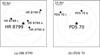 |
Fig. 1 Overviews of the planetary systems of HR 8799 and PDS 70. These overviews use the resonant initial conditions created in Sect. 2.1. |
2 Methods
Simulating a stellar cluster with several planetary systems is computationally expensive. The total simulation time and the time step are determined by the long dynamical timescales of the stellar cluster and the short dynamical timescales of the planetary systems, respectively. The methodology of this work is based on Lonely Planets (Cai et al. 2017) to achieve a reasonable total simulation time.
Lonely Planets solves the problem of perturbations on planetary systems by encounters with neighbouring cluster stars by splitting the problem into two stages. First, we simulated a stellar cluster without any planetary systems and recorded the interaction history of the stars. Then, we assigned an HR 8799 system or a PDS 70 system to a cluster star that matches the mass of the host star of HR 8799 or PDS 70 and integrated the planetary system along with the interaction history of its assigned host star. By splitting the problem into these two stages, we can make more accurate comparisons between different planetary systems because these planetary systems experience identical interaction histories. If the systems experienced slightly different interaction histories, the final conditions may be drastically different as these systems of three or more bodies are chaotic (Miller 1964). Nesvorný & Morbidelli (2012) and Clement et al. (2019) demonstrate the quantitative and qualitative effects that chaos can have on numerical simulations involving giant planets. Furthermore, reusing the interaction history of the stellar cluster saves computing resources and allows us to finish simulations in a shorter amount of time. We further delve into the details of our implementation of Lonely Planets in the following subsections.
2.1 Initial conditions
We simulated a stellar cluster using the integrator Ph4 (Portegies Zwart & McMillan 2018) in the AMUSE simulation framework (Portegies Zwart et al. 2009; Portegies Zwart et al. 2013; Pelupessy et al. 2013; Portegies Zwart & McMillan 2018; Portegies Zwart et al. 2023). We initialised the stellar cluster similar to the Solar birth cluster (Portegies Zwart 2019): 5000 stars in a Plummer sphere (Plummer 1911) with a Plummer radius of 0.7 pc, and with a Kroupa initial mass function between 0.08 M☉ and 100 M☉ (Kroupa 2002). We placed the cluster in a Milky Way potential (Bovy 2015) such that the centre of the cluster follows the modern-day orbit of either HR 8799 or PDS 70. We created the initial conditions using the position, parallax, and motion of HR 8799 and PDS 70 from the Gaia third data release (Prusti et al. 2016; Vallenari et al. 2023) and from Gontcharov (2006). These orbits are relative to the Sun’s galactic orbit (Reid et al. 2014; Karim & Mamajek 2017). We simulated for 10 Myr with a step size of 1 kyr. This period of time is a balance between the cluster’s ability to perturb declining (e.g. through stellar mass loss (Vink 2008)), and provided the planetary systems enough time to be perturbed. We recorded the positions, velocities, masses, and radii of the cluster stars after each step of the simulation.
We preselected the host stars in the cluster by selecting the 50 stars whose masses are the closest to the mass of HR 8799 and PDS 70. This typically results in stars whose original mass was between 1.34 M☉ and 1.52 M☉ for HR 8799, and 0.74 M☉ and 0.78 M☉ for PDS 70. We set the masses of the preselected host stars to be equal to the mass of HR 8799 or PDS 70 before the simulation starts. Otherwise, we would need to change the mass of the host star after the simulation has finished or scale the planetary system to fit the host star’s mass. This would lead to undesired side effects, such as an incorrect interaction history or an altered interaction cross-section. We assigned HR 8799 and PDS 70 their own individual stellar cluster to prevent competition between their preselections and to minimise any influence that setting the mass of the host stars may have. The effects on the initial mass function are negligible as the number of changed host star masses is small enough and the density of the initial mass function around the masses of HR 8799 and PDS 70 is high enough such that all changes to the host star masses are small.
Mass loss due to stellar evolution is important for high-mass stars on the timescale of the simulation (Vink 2008). We accounted for this mass loss by changing the mass of the stars during the cluster simulation using the stellar evolution solver SeBa (Portegies Zwart & Verbunt 1996; Toonen et al. 2012).
We created initial conditions of HR 8799’s planetary system with an MMR chain by initially placing the four planets slightly wider than the 2:1 period ratio from observations (Goździewski & Migaszewski 2020). We then pushed the outermost planet inwards to ensure convergent migration similar to Tamayo et al. (2017), while dampening the eccentricities to match the observations. We integrate this system using REBOUND (Rein & Liu 2012) with WHFAST (Rein & Tamayo 2015). As shown in Fig. 2, the system achieves MMR through the inward migration of the outer planet, so the MMR chain is formed outside-in. We go through a similar process to create PDS 70’s initial conditions from observations of PDS 70 (Wang et al. 2021).
We created non-resonant initial conditions for HR 8799 and PDS 70 by modifying their resonant initial conditions. We considered each planet to be a binary component, whereas the other component is a virtual body. This virtual body represents the combination of the host star and the planets closer to the host star than the considered planet and takes on their combined mass, centre-of-mass position and centre-of-mass velocity. We used a virtual body instead of just the host star itself to account for the effects that close-in planets have on the host star. We then decomposed the binary of the planet and the virtual body into orbital elements, randomised the mean anomaly, and recomposed the modified orbital elements into a binary. Lastly, we adjusted the positions and velocities of the considered planet and the bodies represented by the virtual body according to the changes in position and velocity in the modified binary.
The resulting initial conditions can be found in Table A. 1 for both resonant initial conditions and non-resonant initial conditions. We can verify whether the initial conditions are in MMR or contain an MMR chain using resonance angles (see Appendix B). We assigned copies of both types of initial conditions for each planetary systems to each of the preselected host stars.
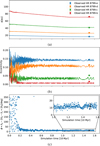 |
Fig. 2 Semi-major axes of the four planets (a), the eccentricities of the four planets (b), and the four-body resonance angle of the planetary system (c) during the initialisation of HR 8799’s initial conditions. The data points with error bars indicate the observed values of the semi-major axes, the eccentricities, and the four-body resonance angle (Goździewski & Migaszewski 2020). |
2.2 Stellar encounters
We took the encounters from the simulated cluster from Sect. 2.1. Determining when a star should be considered an encounter is a complex problem; every star always affects any planetary system due to the infinite range of gravity. Furthermore, the effect of an encounter depends on multiple parameters of the perturbing star, for example: the mass of the perturber, how close the perturber gets, and the relative velocity of the perturber (Hut & Bahcall 1983). We consider a fixed number of six neighbouring stars as perturbers at any given time.
There are multiple ways to choose the neighbours. The simplest way is to choose the stars with the shortest distance to the host star. However, this method introduces the risk that a strong perturber may be obscured by a couple of closer low-mass stars. A more refined approach is to choose the stars that exert the strongest gravitational force on the host star. This mitigates the screening of high-mass stars by low-mass stars, but a stronger gravitational force does not necessarily lead to a stronger perturbation as the host star and its planets experience a near-identical force from the perturber. Therefore, we chose to select perturbing neighbours based on the difference in the force exerted on the host star compared to its planets, i.e. the gradient of the gravitational force at the host star.
We performed our selection using a k-nearest neighbours search (Fix & Hodges 1951) by maximising the selection quantity q. For nearest neighbour and gravitational force selection, these quantities are qn n = 1/r and qF = M/r2, respectively, where any quantities irrelevant to the selection are removed (e.g. constants and properties of the host star). Selecting on distance or gravitational force only involves two bodies (the host star and the candidate neighbour), but the gravitational force gradientbased selection involves at least three bodies as we now have to consider the planetary system of the host star as well. For simplicity, we reduced this scenario to the host star, the candidate neighbour, and the outermost planet being spatially aligned, with the planet located between the stars at a distance d from the host star2, ignoring any other planets. This led to the selection quantity, q∇ F, given by
 (1)
(1)
For human intuition, it can be useful to collapse the equation into a single term. This can be done by assuming that the planet is much closer to its host star than to the candidate neighbour (d ≪ r) using the following expression:
 (2)
(2)
We can again remove the factors that are not properties of the candidate neighbour to get q∇ F ≈ M/r3. The derivative in Eq. (2) shows that selection based on the difference between the gravitational force exerted on the host star and the gravitational force exerted on its planets is approximately equivalent to selection based on the gradient of the gravitational force exerted on the host star.
The dynamical timescale of a planetary system is much smaller than the dynamical timescale of the stars in the stellar cluster. Therefore, we have to either record the data of the stars in the cluster at an unnecessarily high rate or reconstruct the paths of the stars by interpolating the recorded data. We chose to interpolate the recorded data to save on computer resources, as we deemed the recorded cluster data to be recorded densely enough. We performed this interpolation by fitting a fourth order polynomial between adjacent data points of each of the three components of both the positions and the velocities of the stars.
2.3 Integrating the planetary systems
We used the N-body code Symple, which is part of AMUSE3, to integrate the planetary systems because of its symplectic nature, and because the version of REBOUND used before did not support multiple strong perturbers. We configured Symple to use 6th order integration with a time step parameter of 0.01. We ran the simulations for 10 Myr to match the run time of the cluster simulation. We saved a snapshot every 1 kyr to sample the orbit of the least bound outer planet every couple of orbits. These simulations consist of both isolated runs and runs perturbed by neighbouring cluster stars.
At the start of the run, we loaded a planetary system and, if the run was a perturbed run, added its neighbouring stars as determined in Sect. 2.2 relative to the host star of the planetary system. Any present neighbours deviate from their paths in the cluster as most of the cluster is now absent. Therefore, we updated their positions and velocities every 100 yr using the interpolated recorded data from the cluster to correct the deviations. Whenever another star overtook a neighbour, the neighbour was removed and this other star became a neighbour.
An encounter with a neighbouring star or an internal dynamical perturbation may be severe enough that one or more planets are lost. In such a case, we stopped the run. We detected these events after each time step by checking whether any of the planets was both energetically unbound (i.e. its kinetic energy exceeds its gravitational potential energy imposed by the planetary system) and located at least 100 times the initial Hill radius of the initial outermost planet away from the host star. A planet that fulfils both of these conditions could never return to the planetary system. If any planet met these two conditions, the run was ended and the planetary system was considered (partially) destroyed.
3 Results
3.1 Survival time in isolation
For both HR 8799 and PDS 70, we ran a single simulation with resonant initial conditions and 50 simulations with 50 different non-resonant initial conditions. We ran these simulations for up to 10 Myr. The planetary systems were in isolation. The reason for running only a single simulation with isolated resonant initial conditions is that we only had one set of resonant initial conditions. Integrating copies of this set of initial conditions was not useful as isolated simulations of identical initial conditions would produce identical results. We present the results of these simulations in terms of the survival rate over time, fs(t), separately for HR 8799 and PDS 70 in the following subsections. These results show that the resonant initial conditions of both HR 8799 and PDS 70 created in Sect. 2.1 are stable enough to survive the entire 10 Myr in isolation.
3.1.1 HR 8799
The survival rates over time for isolated HR 8799 systems are shown in Fig. 3. The resonant system survives until the cutoff time of 10 Myr, while none of the 50 non-resonant systems do. However, one non-resonant system almost survives until 10 Myr, but dissolves in the last 30 kyr. When inspecting its resonance angles (see Figs. 4 and 5), we see that its randomised mean anomalies are close to MMR. Although near MMR, the system does not form an MMR chain. The semi-major axis differences Δ in terms of mutual Hill radii RH as described by Smith & Lissauer (2009) (who use β instead of Δ) are Δe−d = 3.20 RH, e−d, Δd−c = 2.80 RH, d−c and Δc−b = 3.98 RH, c−b for the consecutive planet pairs of HR 8799 e through HR 8799 b. These semimajor axis differences are well below the instability criterion of Δ<10 RH of Chambers et al. (1996) and Δ ≲ 8.4 of Smith & Lissauer (2009) for multiplanetary systems, and mostly below the instability criterion of  of Gladman (1993, except for Δc−b) for systems with two planets. Therefore, the instability of the non-resonant systems is not unexpected.
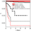 |
Fig. 3 Fraction of surviving planetary systems over time (fs(t)) for HR 8799. The figure shows the isolated resonant system, the 50 perturbed resonant systems, the 50 isolated non-resonant systems, and the 50 perturbed non-resonant systems. In addition, a re-interpretation of the perturbed resonant systems that lost resonance is shown. These systems are shifted in time such that the moment they lose resonance is at t = 0. This subset constitutes 10 HR 8799 systems. All sets of systems display distinct behaviour from one another. The perturbed resonant systems that lost resonance dissolve slower than the non-resonant systems. The curve showing reinterpreted perturbed resonant systems is cut off at 8.8 Myr as we do not have data for the last 1.2 Myr. Later analysis in Sect. 4 shows in Table 1 that the isolated resonant curve and the perturbed resonant curve do not have a statistically significant difference as the difference between 0 and the value for λ for the perturbed resonant systems is not statistically significant. |
3.1.2 PDS 70
The survival rates over time for isolated PDS 70 systems are shown in Fig. 6. The single resonant system survives until the cutoff time of 10 Myr, but unlike HR 8799, 17 out of 50 non-resonant systems survive until the cutoff time of 10 Myr. Similar to the two-body resonance angles of one non-resonant HR 8799 system (Fig. 4), the two-body resonance angles of 15 of these 17 non-resonant PDS 70 systems indicate that the systems are near MMR. This increased fraction of randomly generated MMRs for PDS 70 can be explained by the number of planets in each system: HR 8799 has four planets and PDS 70 has two planets. Therefore, HR 8799 requires three planets to align by chance with their inward neighbour to be fully in MMR, while PDS 70 only requires one planet to do so. The steady decay of non-resonant systems is not unexpected, as the semi-major axis difference, Δ=2.97 RH, is below the instability criterion of  of Gladman (1993) for systems with two planets.
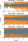 |
Fig. 4 Two-body resonance angles over time of an isolated nonresonant HR 8799 system that is near MMR, starting with the inner planet pair (HR 8799 e and HR 8799 d) and ending with the outer planet pair (HR 8799 c and HR 8799 b). The colours show the use of the argument of pericentre of either the inner planet (blue) or the outer planet (orange). The plots show that the planets are near MMR as the resonance angles are librating. These arguments of pericentre are noisier towards the outer planets as these planets have lower eccentricities. Therefore, the argument of pericentre is more sensitive to change and becomes harder to determine. |
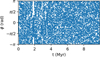 |
Fig. 5 Four-body resonance angle over time of an isolated non-resonant HR 8799 system that is near MMR. The plot shows that the planets do not form an MMR chain as the resonance angle does not librate. |
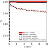 |
Fig. 6 Fraction of surviving planetary systems over time (fs(t)) for PDS 70. The figure shows the isolated resonant system, the 50 perturbed resonant systems, the 50 isolated non-resonant systems, and the 50 perturbed non-resonant systems. In addition, a re-interpretation of the perturbed resonant systems that lost resonance is shown. These systems are shifted in time such that the moment they lose resonance is at t = 0. This subset constitutes three PDS 70 systems. The isolated non-resonant systems and the perturbed non-resonant systems are not distinct from each other. The perturbed resonant systems that lost resonance dissolve much faster than the non-resonant systems. Later analysis in Sect. 4, as shown in Table 1, demonstrates that the isolated resonant curve and the perturbed resonant curve do not differ significantly, since the difference between 0 and the value for λ for the perturbed resonant systems is not statistically significant. |
3.2 Survival time in a cluster
For both HR 8799 and PDS 70, we ran 50 resonant and 50 non-resonant simulations in which the planetary systems were perturbed by their neighbouring stars. We compare the behaviour of these perturbed systems with the behaviour of the isolated systems in Sect. 3.1. In the resonant simulations, we copied the resonant initial conditions 50 times and assigned each copy to a unique host star (see Sect. 2.1). In the non-resonant simulations, we assigned the 50 different non-resonant initial conditions from Sect. 3.1 to the same set of unique host stars. We present the results of these perturbed simulations in terms of the survival rate over time, fs(t), separately for HR 8799 and PDS 70 in the following subsections. We present the subset of the perturbed resonant systems that lost their resonance in order to compare them with the perturbed non-resonant systems. We did this by reinterpreting these systems as non-resonant, individually shifting time so that the moment each system loses resonance aligns across all cases.
3.2.1 HR 8799
The survival rates over time for perturbed HR 8799 systems are shown in Fig. 3. 41 of the 50 resonant systems survive the perturbations from their neighbouring stars, compared to the system that survives in isolation. Curiously, two non-resonant systems now survive until the cutoff time of 10 Myr when perturbed, while none of the non-resonant systems did in isolation. These two systems are the system in Sect. 3.1.1 that almost survived until the cutoff time in isolation, and another system that no longer suddenly dissolves. The first system briefly forms an MMR chain when perturbed by neighbours (see Fig. 7). The second system survives roughly 0.65 Myr in isolation before violently dissolving in the last 20 kyr. In the perturbed simulation, it drastically changes its architecture (see Fig. 8). Similar to the first system, the second system begins near MMR without an MMR chain, but never forms an MMR chain in either simulation and eventually loses its two-body MMRs in the first 2 Myr of the perturbed evolution. Figure 3 shows that not only these two systems survive longer, but that all systems appear to survive systematically longer. The significance of this observation is discussed in Appendix C and the necessary changes to the architecture of the planetary system to explain this observation are further investigated in Appendix D.
The fifth plotted curve of Fig. 3 shows the 11 resonant systems that lost resonance, except for one. One of these 11 systems is omitted because it lost resonance less than 100 kyr before the end of the simulation and managed to survive until the cutoff time. Therefore, the exact survival time after losing resonance is unknown, which may incorrectly skew the fifth curve with an underestimated survival time for this system. Nine of the remaining ten systems that lost resonance do not survive until the end of the simulation. The last system that lost resonance loses resonance after 1.2 Myr and manages to intermittently restore its MMR chain. We cut off the fifth curve at 8.8 Myr as we do not know whether the system would survive the last 1.2 Myr. The other 39 resonant systems maintain their MMR chains and occasionally increase their libration magnitudes in their four-body resonance angles. The resonant systems that lost resonance survive longer from the moment they lose resonance than the perturbed non-resonant systems, as seen by the fifth curve compared to the curve of the perturbed non-resonant systems. This implies that losing resonance is not as harmful to these systems as being out of resonance due to randomised mean anomalies.
The non-resonant systems survive longer when perturbed by their neighbours; 36 systems survived longer compared to 14 systems that survived shorter (see Fig. 9). This asymmetry between longer and shorter survival times tentatively suggests that the survival time of these non-resonant planetary systems increases thanks to perturbations from neighbours.
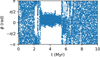 |
Fig. 7 Four-body resonance angle over time of a perturbed non-resonant HR 8799 system that is near MMR. An MMR chain is formed after approximately 3 Myr and is lost after approximately 5.5 Myr, since the resonance angle librates during this range of time. |
 |
Fig. 8 Non-resonant HR 8799 system dissolving after approximately 0.65 Myr in isolation. When perturbed by neighbouring cluster stars, this system nonetheless reached the cutoff time of 10 Myr. The shaded areas indicate the range between each planet’s pericentre and apocentre. Around 1.4 Myr, the system alters its architecture by swapping planets, expanding the orbits of HR 8799 e and HR 8799 c, and shrinking the orbit of HR 8799 d. HR 8799 e and HR 8799 c do not interact despite overlapping areas, as their orbital orientations differ. |
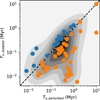 |
Fig. 9 Survival times of the isolated non-resonant systems (Ts, isolated) versus the survival times of the perturbed non-resonant systems (Ts, perturbed) for HR 8799. The systems are biased towards surviving longer when perturbed. The colour of a data point indicates if a system survived longer when isolated (blue, i.e. left of y = x) or survived longer when perturbed (orange, i.e. right of y = x). The background shows a kernel density estimation. |
3.2.2 PDS 70
The survival rates over time for perturbed PDS 70 systems are shown in Fig. 6. Forty-seven of the 50 resonant systems survive the perturbations from their neighbouring stars, compared to the single system surviving in isolation. The number of perturbed non-resonant systems that survive is nearly identical to the isolated non-resonant systems: 19 perturbed non-resonant systems survive until the cutoff time of 10 Myr versus 17 non-resonant systems doing so in isolation, with an overlap of 14 systems. This implies that the non-resonant PDS 70 systems are not strongly influenced by the perturbations of their neighbours. However, Fig. 10 shows that individual survival times can be strongly affected. 15 of the 19 surviving perturbed non-resonant systems start near MMR.
Nineteen non-resonant PDS 70 systems survived longer when perturbed versus 17 non-resonant PDS 70 systems that survived longer when isolated, ignoring the 14 non-resonant PDS 70 systems that survived until the cutoff time of 10 Myr both when isolated and when perturbed. This is in contrast to the non-resonant HR 8799 systems, which appear to favour a perturbed environment. Perturbations from neighbouring stars may help stabilise a broken MMR chain and these perturbations may not do so for just a broken MMR.
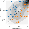 |
Fig. 10 Survival times of the isolated non-resonant systems (Ts, isolated) versus the survival times of the perturbed non-resonant systems (Ts, perturbed) for PDS 70. The systems are not biased towards surviving longer when either isolated or perturbed. The colour of a data point indicates whether a system survived longer when isolated (blue, i.e. left of y = x) survived longer when perturbed (orange, i.e. right of y = x) or survived as long when isolated as when perturbed (green, i.e. on y = x). The background shows a kernel density estimation. |
4 Discussion
The data in Figs. 3 and 6 show that different observationsconformant configurations of HR 8799 and PDS 70 in different environments have different survival times. Further analysis of this data may impose constraints on the architecture of HR 8799 or PDS 70. We model the dissolution of the systems as an exponential decay using the exponential distribution: p(t)=λe−λt for t ≥ 0. This distribution yields the dissolution rate model fd(t)=1−e−λt, which is equivalent to the survival rate model fs(t)=e−λt. Propagation of errors yields a standard deviation of σfd = σfs = fs(t)(tσλ + λσt). We omit the isolated resonant systems in this analysis as we only have one data point available for each planetary system. For n dissolution events at times ti, the parameter λ is estimated by the inverse of the average of the times ti (Ross 2009) using,
 (3)
(3)
with a 1σ confidence interval estimated with
 (4)
(4)
where  and
and  are the values of a χ2 distribution with 2n degrees of freedom where the distribution’s CDF is equal to that of a normal distribution at a value of −1 and +1, respectively.
However, this estimate of λ assumes that all data points are independently drawn from the exponential distribution (i.e. all systems have dissolved), but our data are cut off at a time, Tc. The set of dissolved systems is effectively drawn from a cut-off exponential distribution pc(t) given by
 (5)
(5)
When applying Eq. (3), this yields the following observed expected λobs in terms of the true λ:
 (6)
(6)
which cannot be solved analytically for λ. Consequently, the observed bounds from Eq. (4) also differ from the true bounds (interpreted as a standard deviation σl/u = |λ−Δ λl/u| for a lower or upper bound Δ λl/u) via
 (7)
(7)
We obtain corrected values for λ by solving Eq. (6) numerically and obtain corrected uncertainties for λ by using Eq. (7).
Finally, the expected survival fraction at the age of a system T0 is fs(T0)=e−λT0, which is better suited in terms of the natural logarithm when analysing its error: ln fs(T0)=−λT0. The error on the natural logarithm of this fraction by propagation of errors is  for a normally distributed age and σln fs(T0)=T0 σλ for a boundary age.
λ, ln fs, and a 5 σ confidence interval (CI) of fs of HR 8799 (for a boundary age of both 20 Myr and 50 Myr) and PDS 70 can be found in Table 1. The CIs for HR 8799 show that HR 8799’s planetary system is only expected to survive to its current age if and only if it is in an MMR chain, as the upper bound of the expected survival fraction is negligible for an HR 8799 planetary system that is out of resonance. Perturbed resonant HR 8799 systems can dissolve due to interactions with neighbouring stars, but we cannot rule out with complete confidence that HR 8799 would not survive such an environment, as the upper bound of the expected survival fraction is not negligible for a perturbed HR 8799 planetary system that is in resonance. There exists a little overlap between the resonant and non-resonant CIs. The value for ln fs for the perturbed resonant systems encounters the non-resonant CIs after 3.1σ and 2.9σ for the isolated and perturbed CIs, respectively, and the non-resonant CIs encounter the perturbed resonant CIs after 4.0σ in both cases. From these σ values, the probability that both true values are in the other’s CI is 5.4σ between the perturbed resonant CI and the isolated non-resonant CI, and 5.3σ between the perturbed resonant CI and the perturbed non-resonant CI. Therefore, we believe that the overlap between the CIs should not be an issue.
Although we expect the resonant PDS 70 systems to dissolve less than the non-resonant PDS 70 systems because the means of ln fs prefer the perturbed resonant systems, we cannot with confidence claim anything about the presence of MMR in PDS 70 or the environment of PDS 70 as the upper bounds of all three CIs of the expected survival fraction are not negligible. It is also clear that there is much overlap between the resonant and nonresonant CIs, since the values for ln fs, are within 1σ of each other and are therefore statistically indistinguishable.
λ, ln fs, and 5 σfs CI of planetary systems at certain current ages.
5 Conclusion
We performed numerical simulations of the planetary systems HR 8799 and PDS 70 in order to investigate the existence of an MMR in HR 8799 and to study the effects of perturbations from neighbouring cluster stars on planetary systems in MMR, specifically considering systems with an MMR, an MMR chain, a broken MMR, and a broken MMR chain. We summarise our findings as follows:
The planetary system HR 8799 must have an MMR chain to have survived in its current state to its present age of 20 Myr to 50 Myr. We expect an HR 8799 system without an MMR chain to dissolve before reaching its present age. We argue that it is less probable that HR 8799 still resides in a cluster environment, but we cannot rule this out with absolute certainty;
We argue that it is more probable that the planetary system PDS 70 is in MMR for the system to have survived to its present age of 5.4 ± 1.0 Myr, though we cannot rule out the absence of MMR. Similarly, we argue that it is less probable that PDS 70 still resides in a cluster environment, but we cannot rule this out with absolute certainty;
It is likely that systems with a near-resonant or broken MMR chain survive longer when perturbed by stellar encounters than in isolation. Specifically, for HR 8799 systems with a broken MMR chain, we observe an average increase in survival time of approximately 173% when perturbed by stellar encounters.
The results of the isolated non-resonant systems agree with previous studies on planetary system stability: both the HR 8799 systems and the PDS 70 systems violate their respective stability criteria from Gladman (1993), Chambers et al. (1996), and Smith & Lissauer (2009), and both these systems steadily dissolve when in isolation and out of MMR. Compared to the isolated non-resonant results, the perturbed non-resonant HR 8799 systems are almost certainly more stable than their isolated versions, which would result in a slightly different limit to their stability criterion. However, the perturbed non-resonant HR 8799 systems still dissolve at a rate comparable to the isolated non-resonant HR 8799 systems, and this difference is not observed in the non-resonant PDS 70 systems. This difference is far clearer when comparing non-resonant and resonant systems: despite the stability criteria treating the resonant and non-resonant systems equally, the resonant systems are far more stable than the nonresonant systems. This indicates that the stability criteria based solely on mass, orbital elements, and number of planets may not be sufficient, and that an additional term for MMRs should be included, or a separate class of stability criteria may be required for planetary systems in MMR.
Data availability
All used scripts (except for generating the initial conditions), the initial conditions and the resulting data are available on https://doi.org/10.5281/zenodo.15274962.
Acknowledgements
This work was performed using the compute resources from the Academic Leiden Interdisciplinary Cluster Environment (ALICE) provided by Leiden University. The testing and simulation jobs for this work used computing resources for a total of 125 days, 11 hours, 29 minutes and 37 seconds. On average and rounded up, these jobs used 14 cores on a Xeon Gold 6126 and 23 GB of memory. These jobs spent a total of 705 kWh of energy, which is equivalent to 264 kg of CO2 emission in the Netherlands, according to https://calculator.green-algorithms.org (approximating using a Xeon Gold 6142). This research has made use of the VizieR catalogue access tool, CDS, Strasbourg, France (DOI : 10.26093/cds/vizier). The original description of the VizieR service was published in 2000, A&AS 143, 23. This work has made use of data from the European Space Agency (ESA) mission Gaia (https://www.cosmos.esa.int/gaia), processed by the Gaia Data Processing and Analysis Consortium (DPAC, https://www.cosmos.esa.int/web/gaia/dpac/consortium). Funding for the DPAC has been provided by national institutions, in particular the institutions participating in the Gaia Multilateral Agreement. This work used the Python programming language (Van Rossum & Drake 2009) and the Python packages NumPy (Harris et al. 2020), SciPy (Virtanen et al. 2020), Matplotlib (Hunter 2007), AMUSE (Portegies Zwart et al. 2009; Portegies Zwart et al. 2013; Pelupessy et al. 2013; Portegies Zwart & McMillan 2018; Portegies Zwart et al. 2023) and h5py (Collette 2013).
Appendix A Planetary system initial conditions
Resonant and non-resonant initial conditions.
Appendix B Resonance angles
For a given j−oi: j MMR of order oi between two bodies, we define a two-body resonance angle using their mean anomalies λi and an argument of pericentre  ,
,
where X ∈ {0, 1} indicates whether we use the inner (X = 0) or outer (X = 1) argument of pericentre (Huang & Ormel 2022) in
 (B.1)
(B.1)
For PDS 70, we can simplify this equation because we know that its only MMR is 2:1(j = 2, oi = 1). We can also translate the indices 0 and 1 to the planet labels b and c with
 (B.2)
(B.2)
We can also simplify the equation for HR 8799 since its resonances are all 2:1 with
 (B.3)
(B.3)
We can obtain a three-body resonance angle for HR 8799 by solving for  in the cases of i = i; X = 1 and i = i +1; X = 0 (Huang & Ormel 2022): We can combine the two-body resonance angles of i = i; X = 1 and of i = i+1; X = 0 and solve for
  to obtain a three-body resonance angle for HR 8799 (Huang & Ormel 2022) using
 (B.4)
(B.4)
Lastly, we can sum the three-body resonance angles of i = 0 and of i = 1 to get a four-body resonance angle that describes the entire planetary system of HR 8799 (Goździewski & Migaszewski 2020), and translate the indices 0, 1, 2 and 3 to the planet labels e, d, c and b with
 (B.5)
(B.5)
Appendix C Extended survival of perturbed broken MMR chains
From our simulations, it appears that planetary systems with a broken MMR chain (the non-resonant HR 8799 systems) survive longer when perturbed by neighbouring cluster stars, whereas planetary systems with a broken MMR (the nonresonant PDS 70 systems) are negligibly affected by these perturbations. This suggests that perturbing a broken MMR chain somehow allows a planetary system to survive longer.
The data of HR 8799 (see Fig. 9) do not contain definitive survival times for each non-resonant planetary system as 2 of the 50 perturbed survived until the cutoff time of 10 Myr. However, we can tell whether a system survived longer or not since none of the isolated non-resonant systems survived until the cutoff time. This means that we have a complete dataset to perform a one-sided binomial test. We have 36 out of 50 systems surviving longer when perturbed than when isolated. For the null hypothesis, we assume that the survival time is unaffected by the presence of perturbing neighbours, and therefore the probabilities of surviving longer and shorter are equal; H0: P = 0.5. This one-sided binomial test yields a p-value of 0.0013 for HR 8799, which is equivalent to a 3.22σ result for a standard two-sided normal distribution. The data of PDS 70 (see Fig. 10) are not even complete for this one-sided binomial test as 14 non-resonant systems survived until the cutoff time both when isolated and when perturbed. These 14 systems do not provide any information about whether perturbing neighbours affect the survival time of a system. Therefore, we omit them so we can perform a one-sided binomial test. We are left with 36 non-resonant systems, of which 19 survived longer when being perturbed by neighbouring stars. This results in a p-value of 0.43, which is equivalent to 0.78σ.
Alternatively, we can do a more quantitative analysis anyway. We do this by asserting that the survival time of a non-resonant system that has reached the cutoff time is best estimated by the cutoff time. If the survival time is unaffected by perturbing neighbours, then the data in Figs. 9 and 10 should be evenly spread around y = x. On the other hand, if these perturbations do affect the survival time, the data should be evenly spread around y = αx, where α is greater or smaller than 1, depending on whether isolated systems or perturbed systems survive longer. Each data point in the figure provides an αi, which is equal to Ts,isolated,i/Ts,perturbed,i. However, these α’s do not provide a symmetric space when mirroring over y = x (e.g. y = 3x and y = x/3 yield α = 3 and α = 1/3). Instead, we use β = ln α and βi = ln α to remedy this issue. We can estimate β by taking the mean and standard error of the individual βi’s from our data. This yields β = −1.01 ± 0.23 for HR 8799, equivalent to a 4.45σ deviation from y = x in favour of perturbed systems surviving longer, and β = −0.0045 ± 0.23 for PDS 70, equivalent to a 0.020σ deviation from y = x in favour of perturbed systems surviving longer. We know that the result for HR 8799 is slightly underestimated as only two perturbed non-resonant systems survived until the cutoff time and no isolated non-resonant systems did. It is impossible to know if PDS 70’s result is underestimated or overestimated since a notable fraction of both isolated and perturbed non-resonant systems survived until the cutoff time. If we translate the resulting β values back to α 's, we get that we expect non-resonant HR 8799 systems to survive approximately 173% longer on average and non-resonant PDS 70 systems to survive approximately 0.45% longer on average when either is perturbed by neighbouring stars.
For HR 8799, the one-sided binomial test yielded the weaker of the two results. This is not surprising since it treats each data point as equal, while Fig. 9 shows that the systems that survived longer when perturbed produce more extreme deviations from y = x than the systems that survived longer in isolation. This means that the one-sided binomial test underestimates the effect the perturbations have on the survival times of the systems. This issue is addressed by the more quantitative estimation of β, though at a minor cost to data completeness. The data completeness cost for HR 8799 is small as only two out of 50 systems do not provide complete data, and we know that the result is slightly underestimated because of it. Both tests for HR 8799 agree, so we conclude that wide planetary systems such as HR 8799 with a broken MMR chain survive longer when perturbed by neighbouring cluster stars than when isolated. The 4.45σ result from the estimation of β provides fairly accurate, though conservative, statistical evidence for this conclusion. For PDS 70, neither result is statistically significant, so we can only conclude that there is no indication that the survival times of wide planetary systems such as PDS 70 with a broken MMR are affected by perturbations of neighbouring cluster stars.
Appendix D Non-resonant architectural shifts
As shown in Sect. 3.2.1, perturbations by neighbouring cluster stars may cause a non-resonant HR 8799 system to alter its architecture. This somehow allows the planetary system to survive longer than in isolation. We aim to determine what kinds of architectural shifts are caused by the perturbations and how these changes affect the survival time of a planetary system. We analyse the orbital parameters of both the isolated and the perturbed non-resonant planetary systems of both HR 8799 and PDS 70. Any asymmetry between isolated and perturbed systems or between HR 8799 and PDS 70 could explain the qualitative differences between Figs. 9 and 10.
D.1 HR 8799
As shown in Figs. D.1a and D.2a, the isolated resonant HR 8799 system does not evolve apart from some oscillation around its initial conditions. When the resonant HR 8799 system is perturbed by its neighbours (Fig. D.1b), the effects of the perturbations become visible as noise-like deviations from the initial conditions. The semi-major axes are scattered up to approximately 10000 AU, the eccentricities go up to 1, and significant deviations can be found in the inclinations. An example is shown in Fig. D.2b. However, all these deviations are short-lived, and the single stable mode corresponds to the initial conditions.
The isolated non-resonant systems in Fig. D.1c also have the initial conditions as the dominant mode. Similar to the perturbed resonant systems, the orbital parameters are no longer bound to just the initial conditions as unstable systems get perturbed by self-interaction. However, the semi-major axes only got up to roughly 3000 AU and the inclinations rarely go beyond 1 rad. The perturbed non-resonant systems (see Fig. D.1d) are similar to the perturbed resonant systems, though the noise-like continuum is slightly elevated, which indicates that slightly more systems get perturbed to fill these parts of parameter space. The perturbed non-resonant systems reach the same semi-major axis bound as the perturbed resonant systems of around 10000 AU. Figure D.1d also shows a second apparent stable mode for HR 8799 d and HR 8799 b. However, this mode is explained by the single system in Sect. 3.2.1 that adapted into a seemingly stable configuration early in its lifetime (see Fig. 8), also shown in Fig. D.2c.
Figure D.11 shows that perturbation by a neighbouring cluster star and being out of resonance can produce a variety of changes in the architecture of the HR 8799 systems, and that these changes are rarely stable. The perturbations from neighbouring cluster stars produce wider deviations in semi-major axis than being out of resonance, which can explain the difference between the isolated and perturbed non-resonant systems seen in Fig. 3 and discussed in Appendix C. The wider unstable configurations take longer to complete the necessary orbits to destroy themselves through internal interactions than the less wide unstable configurations. Therefore, the perturbed non-resonant systems that are perturbed up to 10000 AU will manage to survive longer than the isolated non-resonant systems that are perturbed up to 3000 AU.
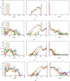 |
Fig. D.1 Histograms of the semi-major axes, eccentricities, and inclinations of the HR 8799 systems, separated by planet. Panel (a): Isolated resonant systems. Orbital evolution oscillates around the initial conditions and the MMR chain is maintained. Panel (b): Perturbed resonant systems. The MMR chain is broken in some simulations. However, these broken MMR chains are often short-lived, so the initial MMR chain remains the only stable mode. Panel (c): Isolated non-resonant systems. Some of the systems diverge from the broken MMR chain and end up destroyed. The eccentricities are not as sharply bound as the resonant systems. Shifts in inclination occur despite the systems being planar and isolated. This should not happen as there is no possible force to drive the planets off the plane. We believe this results from the chaotic growth of numerical errors, as these systems not only live in 2D space, but also are randomly orientated in 3D space. Panel (d): Perturbed non-resonant systems. States that diverged from the broken MMR chain are more prominent than in panels b and c. HR 8799 d and HR 8799 b show an apparent second stable mode, but this only occurs in a single simulation. The broken MMR chain remains the most prominent feature. The dataset of each of the histograms contains all states of all its relevant simulations. These amount to 10000 states per simulation, with one simulation for panel (a), and 50 simulations for panels (b), (c), and (d). By including all states instead of just the final state, longer-lived states become more prominent even if these states are not the final state. |
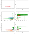 |
Fig. D.2 Paths of semi-major axis versus eccentricity, and semi-major axis versus inclination for a representative set of three different HR 8799 systems. Panel (a): Isolated resonant HR 8799 system. All four planets remain planar and oscillate around their initial semi-major axis and eccentricity. No other changes occur. Panel (b): Perturbed resonant HR 8799 system dissolving before the cutoff time. Only HR 8799 b’s semi-major axis attains some stability after a strong perturbation, before a planet is lost. Panel (c): Perturbed non-resonant HR 8799 system surviving to cutoff, despite dissolving in isolation (see Sect. 3.2.1). Two planets move inwards and two planets move outwards. All planets, except for HR 8799 c (green), remain at their new semi-major axes. The orientations of the orbits are not fixed. |
D.2 PDS 70
Similar to HR 8799, the isolated resonant PDS 70 system does not evolve other than some oscillation around its initial conditions (see Figs. D.3a and D.4a). The data of the perturbed resonant systems in Fig. D.3b show unstable perturbations of semi-major axes going up to 2000 AU, eccentricities up to 1, and inclinations seemingly short-lived above approximately 0.16 rad (for example, see Fig. D.4b). The noise-like continuum of these perturbations that the perturbed resonant HR 8799 systems displayed is far less present in the perturbed resonant PDS 70 systems. The initial conditions remain the dominant mode, even after moderately strong perturbations (see Fig. D.4c).
The isolated non-resonant PDS 70 systems in Fig. D.3c show behaviour that is similar to that of the isolated non-resonant HR 8799 systems: a dominant stable mode around the initial conditions and a noise-like continuum, but up to approximately 10000 AU rather than 3000 AU. Additionally, there is a forbidden valley of semi-major axes for PDS 70 b around the initial orbit of PDS 70 c. Qualitatively, the perturbed non-resonant systems do not differ much from the isolated non-resonant systems other than the existence of non-planar inclinations. The valley for PDS 70 b around PDS 70 c is less pronounced, the level of the noise-like continuum is comparable in width and height, and there are a few apparent stable modes belonging to a single system that maintained these modes for a prolonged period of time.
The figures of HR 8799 (Fig. D.1) and PDS 70 (Fig. D.3) show that both HR 8799 and PDS 70 are affected by nonresonance, but that only HR 8799 is noticeably affected by the perturbations from neighbouring cluster stars as the variety of changes seen in Figs. D.1b and D.1d is not present in Figs. D.3b and D.3d. The non-resonant PDS 70 systems produce similar distributions of semi-major axes up to 10000 AU, since being out of resonance affects PDS 70 far more than perturbations from neighbouring cluster stars. This explains why the divergence between isolated and perturbed non-resonant HR 8799 systems seen in Fig. 3 does not show up for isolated and perturbed non-resonant PDS 70 systems in Fig. 6.
One issue remains with this analysis: HR 8799 and PDS 70 have different interaction cross-sections. The observed difference between HR 8799 and PDS 70 may be explained by wider planetary systems being more affected by the perturbations of neighbouring stars than tighter planetary systems. We can see in Figs. D.1b and D.3b that the noise-like continuum of the perturbed resonant HR 8799 systems is roughly 100 times higher than that of the perturbed resonant PDS 70 systems. The initial semi-major axis of HR 8799’s outermost planet is about a factor of 2 larger than that of PDS 70's outermost planet. This factor of 2 in size equates to a factor of 4 in cross-section, which means that HR 8799 should experience four times more interactions. However, this factor of 4 cannot account for the factor of 100 observed in our data, meaning that the difference in interaction cross-section between HR 8799 and PDS 70 cannot explain the difference in behaviour between HR 8799 and PDS 70. We can only conclude that the number of planets, and therefore the presence of an MMR chain, increases the susceptibility to external perturbations since the number of planets is the only remaining qualitative difference between HR 8799 and PDS 70.
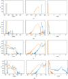 |
Fig. D.3 Histograms of the semi-major axes, eccentricities, and inclinations of the PDS 70 systems, separated by planet. Panel (a): Isolated resonant systems. Orbital evolution oscillates around the initial conditions and the MMR chain is maintained. Panel (b): Perturbed resonant systems. The MMR is rarely broken and any systems with a broken MMR are rapidly destroyed. The inclinations do not diverge far from planar. Panel (c): Isolated non-resonant systems. Some of the systems diverge from the broken MMR. A semi-major axis valley appears for PDS 70 b around the initial semi-major axis of PDS 70 c. The eccentricities are not as sharply bound as the resonant systems. Some of the systems get perturbed violently enough that the direction of PDS 70 b reverses. Despite the issues with random orientations in Fig. D.1c, all systems remain planar here. We believe these systems can manage to stay planar due to a weaker chaotic growth of numerical errors because they contain fewer bodies. Panel (d): Perturbed non-resonant systems. The semi-major axes and the eccentricities are nearly identical to the semi-major axes and the eccentricities in panel c. In contrast to panels (b) and (c), the inclinations are more strongly perturbed and now cover all of the possible parameter space for PDS 70 b. The dataset of each of the histograms contains all states of all its relevant simulations. These are 10000 states per simulation, with one simulation for panel (a) and 50 simulations for panels (b), (c), and (d). By including all states instead of just the final state, longer-lived states become more prominent even if these states are not the final state. |
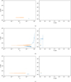 |
Fig. D.4 Paths of semi-major axis versus eccentricity, and semi-major axis versus inclination for a representative set of three different PDS 70 systems. Panel (a): Isolated resonant PDS 70 system. Both planets remain planar and oscillate around their initial semi-major axis and eccentricity. No other changes occur. Panel (b): Perturbed resonant PDS 70 system. The planets lose their MMR due to a perturbation, and no stable orbit is found before a planet is lost. Panel (c): Perturbed resonant PDS 70 system. The planets remain in approximately the same orbits after a perturbation, though tilted and oscillating at a greater magnitude. |
References
- Bovy, J., 2015, ApJS, 216, 29 [NASA ADS] [CrossRef] [Google Scholar]
- Burgasser, A. J., & Mamajek, E. E., 2017, ApJ, 845, 110 [Google Scholar]
- Cai, M. X., Kouwenhoven, M. B. N., Portegies Zwart, S. F., & Spurzem, R., 2017, MNRAS, 470, 4337 [Google Scholar]
- Chambers, J. E., Wetherill, G. W., & Boss, A. P., 1996, Icarus, 119, 261 [Google Scholar]
- Charalambous, C., Cuello, N., & Petrovich, C., 2025, A&A, 696, A175 [NASA ADS] [CrossRef] [EDP Sciences] [Google Scholar]
- Clement, M. S., Kaib, N. A., Raymond, S. N., Chambers, J. E., & Walsh, K. J., 2019, Icarus, 321, 778 [NASA ADS] [CrossRef] [Google Scholar]
- Collette, A., 2013, Python and HDF5 (O’Reilly) [Google Scholar]
- Fix, E., & Hodges, J., 1951, Discriminatory Analysis. Nonparametric Discrimination: Consistency Properties [Google Scholar]
- Gillon, M., Jehin, E., Lederer, S. M., et al. 2016, Nature, 533, 221 [Google Scholar]
- Gillon, M., Triaud, A. H., Demory, B. O., et al. 2017, Nature, 542, 456 [NASA ADS] [CrossRef] [Google Scholar]
- Gladman, B., 1993, Icarus, 106, 247 [Google Scholar]
- Gontcharov, G. A., 2006, Astron. Lett., 32, 759 [Google Scholar]
- Goździewski, K., & Migaszewski, C., 2020, ApJ, 902, L40 [CrossRef] [Google Scholar]
- Griveaud, P., Crida, A., Petit, A. C., Lega, E., & Morbidelli, A., 2024, A&A, 688, A202 [NASA ADS] [CrossRef] [EDP Sciences] [Google Scholar]
- Haffert, S. Y., Bohn, A. J., de Boer, J., et al. 2019, Nat. Astron., 3, 749 [Google Scholar]
- Harris, C. R., Millman, K. J., van der Walt, S. J., et al. 2020, Nature, 585, 357 [NASA ADS] [CrossRef] [Google Scholar]
- Huang, S., & Ormel, C. W., 2022, MNRAS, 511, 3814 [NASA ADS] [CrossRef] [Google Scholar]
- Hunter, J. D., 2007, Comput. Sci. Eng., 9, 90 [NASA ADS] [CrossRef] [Google Scholar]
- Hut, P., & Bahcall, J. N., 1983, ApJ, 268, 319 [NASA ADS] [CrossRef] [Google Scholar]
- Izidoro, A., Schlichting, H. E., Isella, A., et al. 2022, ApJ, 939, L19 [NASA ADS] [CrossRef] [Google Scholar]
- Karim, T., & Mamajek, E. E., 2017, MNRAS, 465, 472 [NASA ADS] [CrossRef] [Google Scholar]
- Keppler, M., Benisty, M., Müller, A., et al. 2018, A&A, 617, A44 [NASA ADS] [CrossRef] [EDP Sciences] [Google Scholar]
- Kroupa, P., 2002, Science, 295, 82 [Google Scholar]
- Laplace, P.-S., 1799, Traité de Mécanique Céleste, https://archive.org/details/traitdemcani01lapl [Google Scholar]
- Laplace, P.-S., 1824, Exposition du Système du Monde (cinquième édition), https://archive.org/details/expositiondusys00lapl [Google Scholar]
- Li, R., Chiang, E., Choksi, N., & Dai, F., 2025, AJ, 169, 323 [Google Scholar]
- Liveoak, D., & Millholland, S. C., 2024, ApJ, 974, 207 [Google Scholar]
- Luger, R., Sestovic, M., Kruse, E., et al. 2017, Nat. Astron., 1, 0129 [Google Scholar]
- Luque, R., Osborn, H. P., Leleu, A., et al. 2023, Nature, 623, 932 [NASA ADS] [CrossRef] [Google Scholar]
- MacDonald, M. G., Ragozzine, D., Fabrycky, D. C., et al. 2016, AJ, 152, 105 [Google Scholar]
- Malhotra, R., 1991, Icarus, 94, 399 [NASA ADS] [CrossRef] [Google Scholar]
- Marois, C., Macintosh, B., Barman, T., et al. 2008, Science, 322, 1348 [Google Scholar]
- Marois, C., Zuckerman, B., Konopacky, Q. M., Macintosh, B., & Barman, T., 2010, Nature, 468, 1080 [NASA ADS] [CrossRef] [Google Scholar]
- Miller, R. H., 1964, ApJ, 140, 250 [NASA ADS] [CrossRef] [Google Scholar]
- Müller, A., Keppler, M., Henning, T., et al. 2018, A&A, 617, L2 [Google Scholar]
- Nesvorný, D., & Morbidelli, A., 2012, AJ, 144, 117 [Google Scholar]
- Pelupessy, F. I., van Elteren, A., de Vries, N., et al. 2013, A&A, 557, A84 [NASA ADS] [CrossRef] [EDP Sciences] [Google Scholar]
- Plummer, H. C., 1911, MNRAS, 71, 460 [Google Scholar]
- Portegies Zwart, S., McMillan, S., Harfst, S., et al. 2009, New Astron., 14, 369 [Google Scholar]
- Portegies Zwart, S., 2019, A&A, 622, A69 [NASA ADS] [CrossRef] [EDP Sciences] [Google Scholar]
- Portegies Zwart, S., & McMillan, S., 2018, Astrophysical Recipes; The art of AMUSE (Bristol, UK: IOP Publishing) [Google Scholar]
- Portegies Zwart, S. F., & Verbunt, F., 1996, A&A, 309, 179 [NASA ADS] [Google Scholar]
- Portegies Zwart, S. F., McMillan, S. L., van Elteren, A., Pelupessy, F. I., & de Vries, N., 2013, Comput. Phys. Commun., 184, 456 [NASA ADS] [CrossRef] [Google Scholar]
- Portegies Zwart, S., van Elteren, A., Pelupessy, I., et al. 2023, https://doi.org/10.5281/zenodo.8409512 [Google Scholar]
- Prusti, T., de Bruijne, J. H. J., Brown, A. G. A., et al. 2016, A&A, 595, A1 [NASA ADS] [CrossRef] [EDP Sciences] [Google Scholar]
- Reid, M. J., Menten, K. M., Brunthaler, A., et al. 2014, ApJ, 783, 130 [Google Scholar]
- Rein, H., & Liu, S. F., 2012, A&A, 537, A128 [NASA ADS] [CrossRef] [EDP Sciences] [Google Scholar]
- Rein, H., & Tamayo, D., 2015, MNRAS, 452, 376 [Google Scholar]
- Ross, S., 2009, Introduction to Probability and Statistics for Engineers and Scientists (Academic Press) [Google Scholar]
- Sepulveda, A. G., & Bowler, B. P., 2022, AJ, 163, 52 [NASA ADS] [CrossRef] [Google Scholar]
- Smith, A. W., & Lissauer, J. J., 2009, Icarus, 201, 381 [NASA ADS] [CrossRef] [Google Scholar]
- Tamayo, D., Rein, H., Petrovich, C., & Murray, N., 2017, ApJ, 840, L19 [CrossRef] [Google Scholar]
- Teyssandier, J., Libert, A.-S., & Agol, E., 2022, A&A, 658, A170 [NASA ADS] [CrossRef] [EDP Sciences] [Google Scholar]
- Toonen, S., Nelemans, G., & Portegies Zwart, S., 2012, A&A, 546, A70 [NASA ADS] [CrossRef] [EDP Sciences] [Google Scholar]
- Vallenari, A., Brown, A. G. A., Prusti, T., et al. 2023, A&A, 674, A1 [NASA ADS] [CrossRef] [EDP Sciences] [Google Scholar]
- Van Rossum, G., & Drake, F. L., 2009, Python 3 Reference Manual (Scotts Valley, CA: CreateSpace) [Google Scholar]
- Vink, J. S., 2008, New Astron. Rev., 52, 419 [CrossRef] [Google Scholar]
- Virtanen, P., Gommers, R., Oliphant, T. E., et al. 2020, Nat. Methods, 17, 261 [Google Scholar]
- Wang, J. J., Vigan, A., Lacour, S., et al. 2021, AJ, 161, 148 [Google Scholar]
- Zink, J. K., Batygin, K., & Adams, F. C., 2020, AJ, 160, 232 [NASA ADS] [CrossRef] [Google Scholar]
Solar System Dynamics. 2024-10-23. Planetary Physical Parameters. https://ssd.jpl.nasa.gov
We can also include the inclination of the planet with respect to the neighbouring star or integrate the force difference over an entire orbit to get more accurate results. However, we prefer this simpler method.
Documentation for Symple will be added in a future iteration of the AMUSE textbook (Portegies Zwart & McMillan 2018).
All Tables
All Figures
|
Fig. 1 Overviews of the planetary systems of HR 8799 and PDS 70. These overviews use the resonant initial conditions created in Sect. 2.1. |
| In the text | |
|
Fig. 2 Semi-major axes of the four planets (a), the eccentricities of the four planets (b), and the four-body resonance angle of the planetary system (c) during the initialisation of HR 8799’s initial conditions. The data points with error bars indicate the observed values of the semi-major axes, the eccentricities, and the four-body resonance angle (Goździewski & Migaszewski 2020). |
| In the text | |
|
Fig. 3 Fraction of surviving planetary systems over time (fs(t)) for HR 8799. The figure shows the isolated resonant system, the 50 perturbed resonant systems, the 50 isolated non-resonant systems, and the 50 perturbed non-resonant systems. In addition, a re-interpretation of the perturbed resonant systems that lost resonance is shown. These systems are shifted in time such that the moment they lose resonance is at t = 0. This subset constitutes 10 HR 8799 systems. All sets of systems display distinct behaviour from one another. The perturbed resonant systems that lost resonance dissolve slower than the non-resonant systems. The curve showing reinterpreted perturbed resonant systems is cut off at 8.8 Myr as we do not have data for the last 1.2 Myr. Later analysis in Sect. 4 shows in Table 1 that the isolated resonant curve and the perturbed resonant curve do not have a statistically significant difference as the difference between 0 and the value for λ for the perturbed resonant systems is not statistically significant. |
| In the text | |
|
Fig. 4 Two-body resonance angles over time of an isolated nonresonant HR 8799 system that is near MMR, starting with the inner planet pair (HR 8799 e and HR 8799 d) and ending with the outer planet pair (HR 8799 c and HR 8799 b). The colours show the use of the argument of pericentre of either the inner planet (blue) or the outer planet (orange). The plots show that the planets are near MMR as the resonance angles are librating. These arguments of pericentre are noisier towards the outer planets as these planets have lower eccentricities. Therefore, the argument of pericentre is more sensitive to change and becomes harder to determine. |
| In the text | |
|
Fig. 5 Four-body resonance angle over time of an isolated non-resonant HR 8799 system that is near MMR. The plot shows that the planets do not form an MMR chain as the resonance angle does not librate. |
| In the text | |
|
Fig. 6 Fraction of surviving planetary systems over time (fs(t)) for PDS 70. The figure shows the isolated resonant system, the 50 perturbed resonant systems, the 50 isolated non-resonant systems, and the 50 perturbed non-resonant systems. In addition, a re-interpretation of the perturbed resonant systems that lost resonance is shown. These systems are shifted in time such that the moment they lose resonance is at t = 0. This subset constitutes three PDS 70 systems. The isolated non-resonant systems and the perturbed non-resonant systems are not distinct from each other. The perturbed resonant systems that lost resonance dissolve much faster than the non-resonant systems. Later analysis in Sect. 4, as shown in Table 1, demonstrates that the isolated resonant curve and the perturbed resonant curve do not differ significantly, since the difference between 0 and the value for λ for the perturbed resonant systems is not statistically significant. |
| In the text | |
|
Fig. 7 Four-body resonance angle over time of a perturbed non-resonant HR 8799 system that is near MMR. An MMR chain is formed after approximately 3 Myr and is lost after approximately 5.5 Myr, since the resonance angle librates during this range of time. |
| In the text | |
|
Fig. 8 Non-resonant HR 8799 system dissolving after approximately 0.65 Myr in isolation. When perturbed by neighbouring cluster stars, this system nonetheless reached the cutoff time of 10 Myr. The shaded areas indicate the range between each planet’s pericentre and apocentre. Around 1.4 Myr, the system alters its architecture by swapping planets, expanding the orbits of HR 8799 e and HR 8799 c, and shrinking the orbit of HR 8799 d. HR 8799 e and HR 8799 c do not interact despite overlapping areas, as their orbital orientations differ. |
| In the text | |
|
Fig. 9 Survival times of the isolated non-resonant systems (Ts, isolated) versus the survival times of the perturbed non-resonant systems (Ts, perturbed) for HR 8799. The systems are biased towards surviving longer when perturbed. The colour of a data point indicates if a system survived longer when isolated (blue, i.e. left of y = x) or survived longer when perturbed (orange, i.e. right of y = x). The background shows a kernel density estimation. |
| In the text | |
|
Fig. 10 Survival times of the isolated non-resonant systems (Ts, isolated) versus the survival times of the perturbed non-resonant systems (Ts, perturbed) for PDS 70. The systems are not biased towards surviving longer when either isolated or perturbed. The colour of a data point indicates whether a system survived longer when isolated (blue, i.e. left of y = x) survived longer when perturbed (orange, i.e. right of y = x) or survived as long when isolated as when perturbed (green, i.e. on y = x). The background shows a kernel density estimation. |
| In the text | |
|
Fig. D.1 Histograms of the semi-major axes, eccentricities, and inclinations of the HR 8799 systems, separated by planet. Panel (a): Isolated resonant systems. Orbital evolution oscillates around the initial conditions and the MMR chain is maintained. Panel (b): Perturbed resonant systems. The MMR chain is broken in some simulations. However, these broken MMR chains are often short-lived, so the initial MMR chain remains the only stable mode. Panel (c): Isolated non-resonant systems. Some of the systems diverge from the broken MMR chain and end up destroyed. The eccentricities are not as sharply bound as the resonant systems. Shifts in inclination occur despite the systems being planar and isolated. This should not happen as there is no possible force to drive the planets off the plane. We believe this results from the chaotic growth of numerical errors, as these systems not only live in 2D space, but also are randomly orientated in 3D space. Panel (d): Perturbed non-resonant systems. States that diverged from the broken MMR chain are more prominent than in panels b and c. HR 8799 d and HR 8799 b show an apparent second stable mode, but this only occurs in a single simulation. The broken MMR chain remains the most prominent feature. The dataset of each of the histograms contains all states of all its relevant simulations. These amount to 10000 states per simulation, with one simulation for panel (a), and 50 simulations for panels (b), (c), and (d). By including all states instead of just the final state, longer-lived states become more prominent even if these states are not the final state. |
| In the text | |
|
Fig. D.2 Paths of semi-major axis versus eccentricity, and semi-major axis versus inclination for a representative set of three different HR 8799 systems. Panel (a): Isolated resonant HR 8799 system. All four planets remain planar and oscillate around their initial semi-major axis and eccentricity. No other changes occur. Panel (b): Perturbed resonant HR 8799 system dissolving before the cutoff time. Only HR 8799 b’s semi-major axis attains some stability after a strong perturbation, before a planet is lost. Panel (c): Perturbed non-resonant HR 8799 system surviving to cutoff, despite dissolving in isolation (see Sect. 3.2.1). Two planets move inwards and two planets move outwards. All planets, except for HR 8799 c (green), remain at their new semi-major axes. The orientations of the orbits are not fixed. |
| In the text | |
|
Fig. D.3 Histograms of the semi-major axes, eccentricities, and inclinations of the PDS 70 systems, separated by planet. Panel (a): Isolated resonant systems. Orbital evolution oscillates around the initial conditions and the MMR chain is maintained. Panel (b): Perturbed resonant systems. The MMR is rarely broken and any systems with a broken MMR are rapidly destroyed. The inclinations do not diverge far from planar. Panel (c): Isolated non-resonant systems. Some of the systems diverge from the broken MMR. A semi-major axis valley appears for PDS 70 b around the initial semi-major axis of PDS 70 c. The eccentricities are not as sharply bound as the resonant systems. Some of the systems get perturbed violently enough that the direction of PDS 70 b reverses. Despite the issues with random orientations in Fig. D.1c, all systems remain planar here. We believe these systems can manage to stay planar due to a weaker chaotic growth of numerical errors because they contain fewer bodies. Panel (d): Perturbed non-resonant systems. The semi-major axes and the eccentricities are nearly identical to the semi-major axes and the eccentricities in panel c. In contrast to panels (b) and (c), the inclinations are more strongly perturbed and now cover all of the possible parameter space for PDS 70 b. The dataset of each of the histograms contains all states of all its relevant simulations. These are 10000 states per simulation, with one simulation for panel (a) and 50 simulations for panels (b), (c), and (d). By including all states instead of just the final state, longer-lived states become more prominent even if these states are not the final state. |
| In the text | |
|
Fig. D.4 Paths of semi-major axis versus eccentricity, and semi-major axis versus inclination for a representative set of three different PDS 70 systems. Panel (a): Isolated resonant PDS 70 system. Both planets remain planar and oscillate around their initial semi-major axis and eccentricity. No other changes occur. Panel (b): Perturbed resonant PDS 70 system. The planets lose their MMR due to a perturbation, and no stable orbit is found before a planet is lost. Panel (c): Perturbed resonant PDS 70 system. The planets remain in approximately the same orbits after a perturbation, though tilted and oscillating at a greater magnitude. |
| In the text | |
Current usage metrics show cumulative count of Article Views (full-text article views including HTML views, PDF and ePub downloads, according to the available data) and Abstracts Views on Vision4Press platform.
Data correspond to usage on the plateform after 2015. The current usage metrics is available 48-96 hours after online publication and is updated daily on week days.
Initial download of the metrics may take a while.