| Issue |
A&A
Volume 700, August 2025
|
|
|---|---|---|
| Article Number | A97 | |
| Number of page(s) | 16 | |
| Section | Numerical methods and codes | |
| DOI | https://doi.org/10.1051/0004-6361/202554298 | |
| Published online | 12 August 2025 | |
Going Bayesian on the ages of nearby young stellar systems
I. The expansion rate method
1
Departamento de Inteligencia Artificial, Universidad Nacional de Educación a Distancia (UNED),
c/Juan del Rosal 16,
28040
Madrid,
Spain
2
Depto. Estadística e Investigación Operativa, Universidad de Cádiz,
Avda. República Saharaui s/n,
Cádiz,
11510
Puerto Real,
Spain
3
Laboratoire d’astrophysique de Bordeaux, Univ. Bordeaux,
CNRS, B18N, allée Geoffroy Saint-Hilaire,
33615
Pessac,
France
★ Corresponding author: This email address is being protected from spambots. You need JavaScript enabled to view it.
Received:
27
February
2025
Accepted:
5
June
2025
Abstract
Context. Determining the ages of young stellar systems is fundamental for testing and validating current star-formation theories. Aims. We aim to develop a Bayesian version of the expansion-rate method that incorporates the a priori knowledge of the stellar system’s age and solves some of the caveats of the traditional frequentist approach.
Methods. We upgraded an existing Bayesian hierarchical model with additional parameter hierarchies that include, amongst others, the system’s age. We propose prior distributions inspired by literature works.
Results. We validate our method on a set of extensive simulations mimicking the properties of real stellar systems. In stellar associations between 10 and 40 Myr and up to 150 pc; the errors are <10%. In star forming regions up to 400 pc, the error can be as large as 80% at 3 Myr, but it rapidly decreases with increasing age.
Conclusions. The Bayesian expansion-rate methodology that we present here offers several advantages over the traditional frequentist version. In particular, the Bayesian age estimator is more robust and credible than the commonly used frequentist ones. This new Bayesian expansion-rate method is made publicly available as a module of the free and open-source code Kalkayotl.
Key words: methods: statistical / open clusters and associations: general / solar neighborhood
© The Authors 2025
 Open Access article, published by EDP Sciences, under the terms of the Creative Commons Attribution License (https://creativecommons.org/licenses/by/4.0), which permits unrestricted use, distribution, and reproduction in any medium, provided the original work is properly cited.
This article is published in open access under the Subscribe to Open model. This email address is being protected from spambots. You need JavaScript enabled to view it. to support open access publication.
1 Introduction
Accurate and precise age determinations of young stellar systems are fundamental elements in the validation of star-formation theories. To this end, the nearby and young stellar systems (NYSSs) are fundamental benchmarks because they offer the best quality data and are more likely to preserve the initial conditions of the star-formation processes. However, inferring the age of these systems is a difficult task due to the often inconsistent results obtained from different dating techniques (see, for example, Galindo-Guil et al. 2022; Barrado y Navascués et al. 1999; Stauffer et al. 1995). Among the various dating techniques that could be used in NYSSs, dynamical ages, such as the expansion-rate method e.g. Wright et al. 2024; Mamajek & Bell 2014; Brown et al. 1997 and traceback method e.g. Galli et al. 2023; Miret-Roig et al. 2022 are fundamental because they provide independent age estimates from those given by other methods, such as isochrone-fitting or a lithium-depletion boundary (see, for example, Ratzenböck et al. 2023; Jeffries et al. 2023; Galindo-Guil et al. 2022; von Hippel et al. 2006, and references therein).
The dynamical dating techniques make the underlying assumption that young stellar systems were more spatially compact at their birth time and that their current size can be mapped to their birth size using the current positions and velocities of their members. The system’s age is thus the time needed for its members to pass from their original configuration to the current one. In the traceback method, the mapping is done by tracing the system’s member's current positions back in time based on their velocities and assuming a Galactic potential. On the other hand, in the expansion-rate method, the mapping is done assuming that the current positions and velocities of the system's members are the consequence of a free expansion at a constant rate. This rate measures the average change in the members' velocity with respect to the distance to the system's centre (see, for example, the section “The concept of linear expansion” in Blaauw 1964. Thus, the expansion rate is a spatial rate rather than a temporal one.
In the expansion-rate dating method, the expansion rate, κ, is inverted to obtain an estimate of the stellar system’s age, τ, through the following equation:
 (1)
(1)
with τ and κ given in units of Myr and km s −1 pc −1, respectively.
We notice that this method makes the underlying assumption that the stellar system is expanding, that this expansion originated at the system's birth, and that it has remained constant since then (see assumptions 1, 2, and 3).
In this work, we revisited the expansion-rate method and provide the community with a Bayesian implementation of it in the form of a module for the free and open-source code Kalkayotl (Olivares et al. 2025). The statistical problem of inverting the probability distribution of the expansion rate to obtain a distribution of the age shares similarities with that of inverting parallaxes to obtain distances (Bailer-Jones 2015), and thus it strongly benefits from a Bayesian approach, particularly in the domain of a low signal-to-noise ratio, as is the case of the expansion rates of NYSSs.
The rest of this work is organised as follows. In Sect. 2, we present the synthetic datasets that we will use to validate our new Bayesian dating method. Section 3 describes the traditional frequentist expansion-rate dating methods and their caveats and introduces our new Bayesian approach with its various priors and hyper-parameters. Then, in Sect. 4, we present a series of sensitivity analyses to select the optimal configurations for the prior distributions and hyper-parameters of our model that maximise its performance. Afterwards, in Sect. 5, we validate the optimal configuration of our method with synthetic datasets of NYSSs. Finally, in Sects. 6 and 7, respectively, we discuss the advantages and limitations of our new Bayesian method and present our conclusions and general recommendations for its use. In addition, Appendix A provides a comprehensive list of the assumptions we made in the construction of our new dating method together with criticisms of each of them.
2 Data
In this section, we present the data that will be used to validate our Bayesian expansion-rate method. We started by establishing the parameter space of the method, that is, its applicability domain, together with a grid of sensible values for it. Afterwards, we describe the characteristics of the synthetic data generation mechanism. Finally, we describe the properties of the synthetic systems that will remain fixed (i.e. those not in the grid of parameter space values), which will be based on archetypical ones.
2.1 Applicability domain
The applicability domain of the expansion-rate method has been poorly characterised in the literature. Brown et al. 1997 first characterised the caveats of a version of the expansion-rate dating method in which the expansion rate of the stellar system is determined from the rate of change of the proper motions of its members with respect to their sky positions. The authors concluded that the kinematic ages determined with this method are limited by the uncertainties in the proper motions and parallax and that the ages determined can be underestimated or overestimated depending on the chosen coordinate direction. Furthermore, they found that their ages eventually converge towards a value of ~4 Myr for associations older than this age, thus indicating that the applicability domain of their expansion rate method is age-dependent and saturates at 4 Myr. Recently, Zari et al. 2019 determined kinematic ages in Orion using a restricted version of the Lindegren et al. 2000 model in which the expansion is assumed isotropic and does not include rotations or shear terms. In their Appendix A.2, those authors used simulated data mimicking the Gaia properties to show that their model can retrieve the expansion parameter in a Hyades-like cluster but underestimate it in an Orion-like one, thus indicating that the applicability domain of the expansion-rate method is distance dependent. These two previous works indicate that the applicability domain of the expansion-rate method depends on the age and distance of the stellar system.
In this work, we inferred expansion ages through a forwardmodelling method in which the age, expansion rates, positions,and velocity dispersions are inferred from an extension to the linear velocity-field model of Lindegren et al. 2000, see Sect. 3). This Bayesian hierarchical model with a linear velocity field is implemented as part of the Kalkayotl code Olivares et al. 2025 , which was thoroughly validated through a set of synthetic data simulations mimicking the properties of Gaia DR3 data. The results of those simulations, particularly those about the detectability of the linear velocity field entries (see Sect. 3.1.2 of Olivares et al. 2025), show that the signal-to-noise ratio of the expansion-rate components not only depends on the age (i.e. the strength of the expansion signal) and distance of the system but also in its number of stars. Moreover, the three values of the C constant shown in Figure 3 of the aforementioned authors can be converted to expansion ages using Eq. (1), resulting in ages of ~100 Myr (C = 10 m s −1 pc −1), ~20 Myr (C = 50 m s−1 pc−1), and ~10 Myr (C = 100 m s−1 pc−1), which correspond to the typical ages of young open clusters, stellar associations, and starforming regions, respectively. Therefore, from this figure, we can conclude that even with a very relaxed threshold of a S/N of 1, the expansion-rate method would not work in open clusters.
Based on the previous analysis, we conclude that a sensible parameter space to probe the applicability domain of the expansion-rate method could be split into two regimes: on one hand, stellar associations with ages between 10 Myr and 50 Myr and distances up to ~200 pc; on the other hand, star-forming regions with ages of <10 Myr and distances up to ~500 pc. The typical populations of stellar associations vary between 20 and 80 members (see, for example, Table 1 of Gagné et al. 2018), while those of star-forming regions are usually in the hundreds (see, e.g. the cases of ρ-Ophiuchi and Taurus in the aforementioned table).
2.2 Generation of synthetic stellar systems
We generated synthetic datasets with the Amasijo1 code (see for example Olivares et al. 2023b; Casamiquela et al. 2022. This free and open-source code takes as input astrometric and photometric parameters together with a random seed generator and the total number of desired system members. These inputs are used to generate the phase-space coordinates and masses of the stellar system's members with a variety of statistical distributions. Here, we assume uniform and multi-variate normal distributions for the masses and phase-space coordinates, respectively. A normal distribution suffices to describe the phase-space distribution of the majority of the known stellar associations and subgroups within star-forming regions. We choose to sample masses from a uniform distribution rather than other forms of the initial mass function to directly constrain the fraction of sources with observed radial velocity using a lower mass limit that translates into a photometric limit. In dynamical age determinations Galli et al. 2023; Miret-Roig et al. 2020;Zari et al. 2019, the coverage of radial velocities is more important than the completeness of the mass function.
Once the phase-space coordinates and masses were generated, they are transformed to the observable space using PyGaia2 and isochrones3 (Morton 2015). The isochrones code generates the true values of the Gaia observed photometry based on the source's mass, distance, metallicity, extinction, and input age. Throughout this work, we set the metallicity to the solar value and extinction to zero. These choices reflect the values of the majority of the stellar associations in the solar neighbourhood. In the case of star-forming regions, a higher extinction would be roughly equivalent to a degradation of the astrometric uncertainty, and thus it is similar to placing the system further away.
Amasijo then uses the PyGaia code to obtain the observational uncertainties for the desired Gaia data release according to the true astrometric, photometric, and radial-velocity values. Finally, the observed values are sampled from univariate normal distributions in which the true values are the mean and the uncertainties the standard deviations. The output of the code consists of a comma-separated-value file with the observed and true values of the generated sources and a plot with a summary of the synthetic data properties.
Additional parameters of the Amasijo code are the fraction of sources with observed radial velocities, the maximum phasespace Mahalanobis distance of the sources, and a magnitude shift to increase the astrometric uncertainties. The synthetic astrometric uncertainties provided by PyGaia are much smaller than those observed in real stellar stellar systems; thus, we applied this magnitude shift to increase the astrometric uncertainties and match the real ones. The maximum phase-space Mahalanobis distance is useful for avoiding sources that were generated by simple random effects at unplausibly large phase-space distances. Throughout this work and in all our simulations, we used a maximum Mahalanobis distance of two, which covers 95% of the phase-space distribution. We set the uncertainty properties to that of the third Gaia data release. The remainder of the parameters were varied with the subsequent grid's values.
Finally, prior to the use of our datasets, we applied the following filtering criteria. First, we filtered out sources with a parallax smaller than 1.0. This effectively removes distant sources that may have resulted from extreme random number generation. Second, we set a lower limit of 100 m s −1 as the minimum radial velocity uncertainty, and thus, the uncertainty of sources with higher precision was fixed to this minimum value. Third, we applied the sigma clipping of sources farther away than three and two standard deviations in parallax and radial velocity, respectively.
2.3 Parameter space grid
We generated stellar systems mimicking the phase-space parameters of archetypical stellar systems: the β-Pictoris stellar association and the Taurus star-forming region. We selected these benchmark systems due to their proximity and well-characterised properties. For β-Pictoris, we used the phase-space parameters inferred by Miret-Roig et al. (2020, see their Table 4), with the position dispersion σXYZ = [16.04,13.18,7.44] pc, velocity dispersion σUVW = [1.49,0.54,0.70]km s−1, and the nominal (i.e. measured) distance and age values of 51 pc (Miret-Roig et al. 2020) and 23 ± 8 Myr (Lee et al. 2024), respectively. We chose the latter work because it is the latest one with an age determination that covers the majority of the literature ones. For the Taurus star-forming region, we used the phase-space centroid parameters of the L1495 subgroup inferred by Galli et al. 2019, see their Tables 2 and 3). In this last case, we set the phase-space dispersion to 1 pc in position and 1 km s−1 in velocity, which correspond to the typical values of the Taurus subgroups and also to those of the NGC1333 and IC348 core subgroups of the Perseus star-forming region (Olivares et al. 2023a).
We replicated the benchmark phase-space templates of β-Pictoris and Taurus L1495 over the grid of values shown in Table 1. We notice that the position and velocity dispersions shown in the last two rows represent the single vector value used to generate the template of either stellar associations or star-forming regions, and these values were not varied throughout our analysis, except in the experiments shown in Sect. 4.3. The ages and distances cover the applicability domain interval discussed in Sect. 2.1, while the number of sources covers the expected population sizes of the majority of the nearby young stellar associations and star-forming regions Gagné et al. 2018. We used low, medium, and high fractions of radial velocity coverages to test the impact that current and dedicated radial velocity surveys may have on our method. Finally, we avoid drawing conclusions from possible random excursions of the random number generator by generating each grid point five times with different random seeds. We generated the benchmark templates with different ages and distances by shifting the distance vector along its nominal direction and by isotropically fixing the expansion-rate components to the requested age using Eq. (1), respectively.
Parameter values for grid of synthetic simulations.
3 Methods
In this section, we introduce the Bayesian method that we propose to infer the ages of NYSSs based on their expansion rate. We start with a review of the current frequentist approach to this dating method. Then, we expose our novel Bayesian approach, together with its associated model and descriptions of its practical implementation and prior distributions.
3.1 Frequentist approach
Traditionally, the frequentist procedure to obtain ages is the following. First, the expansion rates are inferred with maximum likelihood methods (e.g. Luhman 2023, Zari et al. 2019; Wright & Mamajek 2018; Mamajek & Bell 2014; Belikov et al. 2002), where the fits are performed directly on the observed spaces (i.e. proper motions and sky positions, e.g. Belikov et al. 2002), in the physical ones (i.e. space positions and velocities, e.g. Luhman 2023, Zari et al. 2019; Mamajek & Bell 2014) or in combinations of them (e.g. Wright & Mamajek 2018). These fits are independently performed in one or several orthogonal directions (e.g. radial velocity vs. distance or U vs. X, V vs. Y, and W vs. Z), with the correlations between these directions usually disregarded. It can also be assumed that the expansion is uniformly isotropic, as done by Zari et al. (2019). If the procedure results in more than one expansion rate component, a variety of criteria are used to combine them. These criteria go from discarding components (typically in the Z direction, e.g. Mamajek & Bell 2014) to mixing them assuming that they are independent and identically distributed (iid). This latter assumption is at the core of the weighted mean procedure, which is typically used to combine the expansion rates of orthogonal directions (e.g. Luhman 2023; Mamajek & Bell 2014). Finally, once a single estimate of the expansion rate is derived, the system's age is obtained through Eq. (1).
The previous traditional approach, to which we refer hereafter as the classical frequentist method (represented with the symbol κ̂), suffers due to the following caveats. First, it underestimates uncertainties. The fact that the expansion-rate vector, κ, can be decomposed in its orthogonal components  , does not necessarily mean that they are statistically uncorrelated. As is widely known, neglecting correlations results in underestimated uncertainties Gelman et al. 2014). Second, the inversion of a noisy estimate of the expansion rate, κ̂, may result in a biased age estimate in a similar way to that in which the inversion of a noisy estimate of the parallax results in a biased distance estimate (Bailer-Jones 2015).
The last caveat of the classical method can be partially mitigated by only combining and inverting those components of the expansion rate with a sufficient signal-to-noise ratio, for example, S/N>3. Hereafter, we refer to this approach as the robust frequentist method. We notice that the robust method still suffers from underestimated uncertainties due to the neglect of correlations.
3.2 Bayesian approach
From our perspective, the problem of inverting the expansion rate to derive an expansion age has a strong statistical resemblance to the problem of inferring an object's distance by inverting its observed parallax. As demonstrated by the works of Bailer-Jones (2015, 2023), and Bailer-Jones et al. (2021, 2018), the Bayesian approach offers strong advantages to the distanceinference problem. Therefore, in the following, we pose the expansion age inference problem under a Bayesian framework in which we address the caveats of the traditional approach: neglected correlations, underestimated uncertainties, and biased ages.
We used the Bayesian hierarchical modelling formalism Gelman et al. 2014) to propagate data correlations and uncertainties towards the expansion-rate components (i.e. κX, κY, and κZ). Then, the latter were pooled together and inverted to obtain a single age estimate.
3.2.1 Bayesian expansion-age model
In our statistical generative model framework, the age parameter, τ, was inferred as a random variable, which was sampled from its prior (more below) and transformed into the expansion rate, κµ, using the relation, κµ [km s−1 pc −1] = (1.02271 τ[Myr])−1. Then, this κµ was used as the location parameter of a statistical distribution (more below) from which the three κ components (i.e. κX, κY, and κZ) were sampled. These components were then inserted into the Lindegren et al. 2000 linear-velocity model,
 (2)
(2)
in which xi and ui are the position and velocity vectors of member i in the reference frame of the stellar system, x0 and u0 are the position and velocity vectors of this later, Σv is the velocity dispersion covariance matrix of the assumed multi-variate-normal distribution N, and Ω is the set of velocity tensor entries related to the system's rotation and shear. The resulting extended linear velocity field model was implemented in the 6D version of Kalkayotl (Olivares et al. 2025, where the posterior distribution of all its parameters (including the system's expansion age τ, κµ, κσ and other additional parameters) is sampled using the NUTS algorithm (Hoffman & Gelman 2011) within the PyMC environment (Oriol et al. 2023). The diagnostics and summaries of the specific age model parameters were seamlessly incorporated in the standard output of the Kalkayotl code.
The hierarchical approach described above solves the two caveats of the traditional frequentist approach in the following ways. First, by drawing the three expansion-rate components from the same parent distribution and sampling the parameters of this latter with the NUTS method their correlations were directly propagated towards the parameters of the upper hierarchies. Second, the pooling of the three components into a single parameter, κµ, increases the statistical significance of the latter and diminishes the bias that may be incurred when inverting it. Finally, when the parameters of a Bayesian hierarchical model are sampled with the NUTS method, the data uncertainties are fully propagated towards the parameters in upper hierarchies, particularly towards the age parameter. This full propagation avoided the typical problem of an uncertainty leak that occurs when successive trimming is applied to the tails of the parameter's distributions when they are propagated through the chain of steps involved in the expansion age computation. For example, it is typically assumed that the uncertainties in the phase-space coordinates are Gaussian, that the uncertainties in the expansion-rate components are Gaussian, and that the inversion of a Gaussian distribution results in a Gaussian one, none of which is necessarily true.
3.2.2 Prior distributions
We now describe the prior distributions and parametrisation used for the additional age model parameters as well as additional marginal prior distributions for the position and velocity dispersions: σXYZ and σUVW (see Table 2). The rest of the linear velocity model parameters and their prior distributions were left untouched.
The age estimates of NYSS are generally reported in the literature either as intervals or as Gaussian distributions, with a mean and a standard deviation. Therefore, our prior distribution for the age parameter, τ, must have the following two minimum requirements: (i) positive support; and (ii) free and independent mode and variance parameters. Although there is a large variety of family distributions with positive support (e.g. gamma, chisquared, exponential, and all the log-type families) their variance and mode are generally linked, thus rendering their independent specification a task that cannot always be solved. For example, in the chi-squared distribution with k degrees of freedom, the mode and the variance are max(k −1 2,0) and 2k, respectively, which cannot be set independently. Thus, from the set of family distributions that fulfil the above criteria, we chose to work with the truncated normal (on the positive reals) and the generalised gamma (Stacy 1962) (see Table 2).
The truncated normal (TN) distribution offers the most direct way to embed the a priori literature knowledge on the age of a stellar association as a prior by directly passing the mode, µτ, and standard deviation, στ, collected from the literature as hyper-parameters. On the other hand, the generalised gamma distribution has enough flexibility to accommodate varying values of the mode, variance, and skewness. Fixing its parameters to the set of values shown in Table 2 renders distributions with the same mode and variance as a Gaussian distribution, which enabled us to directly convey the a priori knowledge from the literature with the mode, µτ, and standard deviation, στ4. However, the resulting location hyper-parameter must be positive (if this condition cannot be fulfilled, a truncated normal prior should be used instead). The two sets of hyper-parameter values shown in Table 2 for the generalised gamma distribution result in positive and negatively skewed distributions, which for simplicity we call generalised gamma right (GGR) and generalised gamma left (GGL), respectively. Figure 1 compares the three age prior distributions for the case of the β-Pictoris stellar association, where we used the 23 ± 8 Myr reported by Lee et al. (2024). As can be observed, the generalised gamma with positive skewness has a larger positive tail and a sharp cut at younger ages.
As mentioned above, the three expansion-rate components κX, κY, and κZ are drawn from the same statistical distribution, for which we used either a normal or a StudentT distribution, with location κµ, scale κσ, and, in the case of the StudentT, degrees of freedom κν (see Table 2). The sampling can be done with two types of parametrisation: central or non-central. In the central one, the parameters are directly drawn from the distribution, while in the non-central one, first a latent random variable, η, is sampled from the standardised distribution (i.e. location and scale set to 0 and 1, respectively), and then κ = κμ + η · κσ. This latter type of parametrisation is sometimes useful to improve the performance of the NUTS algorithm.
We included the normal and StudentT distributions as prior for the κ components. While the normal distribution helps gather information when the expansion is isotropic, the StudentT helps (with its long tails) in the non-isotropic cases by treating the most discrepant κ component as an outlier. This is typically the case of the κZ component in NYSSs older than 10 Myr due to the effects of the Galactic potential, which, on short timescales, acts primarily in this direction. For example, in β-Pictoris, both Mamajek & Bell (2014) and Miret-Roig et al. (2020) found expansion in the κX and κY components and contraction in κZ, whereas in TW Hydrae, Luhman (2023) found isotropic expansion, with ages of 9.5 Myr, 9.8 Myr, and 9.6 Myr in the X, Y, and Z, directions, respectively.
As a prior for the degrees-of-freedom parameter in the StudentT distribution, we used a gamma distribution, which is the one recommended by Juárez & Steel (2010). Here, we set the hyper-parameters α = 2 and β = 1 resulting in a mode at dof = 1, at which the StudentT distribution reduces to the Cauchy distribution. The long tails of the latter help in the non-isotropic expansion cases.
We set the exponential distribution as prior for the κσ parameter because it imposes a higher probability density on smaller dispersions. This exponential distribution helps to minimise the dispersion between the three κ components, which is the expected behaviour if the association expands isotropically. We notice that rather than imposing isotropic expansion (like, for example, Zari et al. 2019), the exponential prior simply specifies this isotropy as the most probable case.
We included three types of family distributions as priors for the marginal position and velocity dispersions: the TN, exponential, and gamma distributions. The latter is the default one in Kalkayotl’s linear-velocity model. We notice that these distributions were used as marginal priors for each of the three entries of the position and velocity dispersion vectors σXYZ and σUVW. We tested two options as hyper-parameter values for these prior distributions: a generic one and an informed one. The generic one, which is shown in Table 2, uses the typical values for stellar associations and star-forming regions, which are 20 pc in position dispersion and 0.5 km s−1 in velocity dispersion (see, for example, Table 9 of Gagné et al. 2018). On the other hand, the informed option uses the a priori values of the system’s position and velocity dispersions. Throughout the following sections, we use the informed phase-space dispersion prior with the values shown in the last two rows of Table 1 (except in Sect. 4.3). In general, users of our expansion method can set the location hyper-parameters of this phase-space dispersion prior to values that were inferred by previous studies or by them with Kalkayotl’s Gaussian model with joint positions and velocities (see Sect. 2 of Olivares et al. 2025).
Prior distribution for age model parameters.
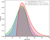 |
Fig. 1 Comparison of our age prior distributions. The hyper-parameters (µτ and στ) were fixed to values that result in a distribution with mode and variance corresponding to those for the β-Pictoris stellar association, 23 ± 8 Myr (Lee et al. 2024). |
4 Sensitivity analysis
Once our Bayesian hierarchical model was specified, we performed a series of sensitivity analyses to choose its optimal configuration (i.e. the combination of prior distributions, parametrisation, and hyper-parameters that renders the most performant age-dating method). Once determined, we used it to evaluate the method’s performance under some deviation conditions. To achieve these goals, we first defined a series of metrics that we used to objectively compare different model configurations. Then, we applied our method with its various configurations to a set of synthetic datasets where the true age is known. We generated these synthetic datasets mimicking the properties of the benchmark β-Pictoris stellar association at its nominal age and distance (see Sect. 2). For simplicity reasons, we kept the fraction of observed radial velocity at 1.0.
As metrics to evaluate our model, we used error, uncertainty, and credibility, all in percentage units. The error measures the relative deviation of the inferred posterior mean with respect to the true value. We notice that this error can be positive or negative depending on whether the inferred mean overestimates or underestimates the value. The uncertainty measures the relative standard deviation of the inferred posterior with respect to the true value. The credibility measures the fraction of synthetic simulations (for each particular case of the grid’s parameter values) for which the true value is contained within the 95% high-density interval (HDI) of the inferred posterior distribution. Finally, the optimal model configuration will be the one that minimises the error and the uncertainty and maximises the credibility, with priority on credibility, error, and uncertainty.
In the following sections, we identify the optimal configurations of our model and then use them to analyse their sensitivity to extreme conditions. First, we evaluate the model performance under shitting and scaling of the prior information. Then, we test the sensitivity of our model to varying phase-space dispersions of the stellar system. Finally, we test our model’s ability to recover the input true age under non-isotropic expansion. These series of experiments will allow us to quantify the biases that our method has when applied to stellar systems deviating from the ideal conditions of unbiased prior age estimates, well-characterised velocity dispersions and isotropic expansion.
4.1 Sensitivity to prior distribution and hyper-parameters
We applied the model configurations described in Sect. 3.2.2 to the synthetic dataset of β-Pictoris. Then, we compared the results based on the previously described metrics and arrived at the conclusions detailed in the following paragraphs.
Concerning the position and velocity dispersions, we found that both hyper-parameter options (i.e. generic and informed) return similar metrics in all parameters, although the informed one minimises the age error by ∼2%. Thus, we recommend using the informed option. We notice that this option cannot be set as the default one in the Kalkayotl code because it is systemspecific, thus, the generic option remains the default. From the three tested family distributions for the position and velocity dispersions (i.e. TN, gamma, and exponential), the ones that minimise the errors and uncertainties are gamma for positions and exponential for velocity. Therefore, we recommend their use and set them as default options.
Regarding the scale hyper-parameter of the exponential prior distribution of κσ, we tested values of scale ∈ [0.001,0.005,0.01]km s−1 pc−1, which roughly correspond to age dispersions similar to 0.1, 0.5, and 1 Myr among the κ components. The three cases result in 100% credibilities, low errors (#x003C;3%), and uncertainties of 11%, 13%, and 15% for the smallest to largest dispersions, respectively. Therefore, we recommend the use of the smallest dispersion and set it as the default option.
With regard to the normal and StudentT distributions that we used to sample the κ components, we observe that both result in 100% credibilities, low errors (<2%), and small uncertainties (<16%). The only difference we notice between the results of these two distributions is that the normal one produces lower errors (1% vs. 2%) in systems with 25 sources, while in more populated systems the error resulting from the StudentT case diminishes. Therefore, we recommend the use of the normal default configuration when there is evidence of isotropic expansion, which can be gathered by running Kalkayotl with the linear-velocity model without the expansion age module. In Sect. 4.4, we further evaluate the performance of these two distributions on stellar systems with non-isotropic expansion.
Concerning the parametrisation of κ, we tested central and non-central cases, with them having errors <3% and ∼7%, respectively. The uncertainties of the central parametrisation are 1% smaller than the non-central one. Therefore, we recommend the use of the central parametrisation and we set it as the default one within Kalkayotl.
Figure 2 shows the metrics of the age prior experiments.Concerning the tested prior distributions for the age parameter (i.e. TN, GGR, and GGL), the GGR had convergence issues that resulted in large errors (~ –30%) and low credibilities ( ~80%) most probably due to the sharp cut that it applies to younger ages (see, e.g. Fig. 1). On the contrary, TN and GGL resulted in 100% credibilities, with the GGL showing the smaller errors (≲3%) and uncertainties (<16%), compared to those of the TN, which are 10% in error and<19% in uncertainty. Therefore, we conclude that the GGL distribution globally outperforms the TN. For this reason, we recommend its use and set it as the default option.
In the following, we refer to the previous optimal configuration of hyper-parameters and prior distributions as the default-age model, and we denote it as Default(·). Whenever we use a different configuration, we explicitly state its difference from the default one. For example, when using a configuration in which the StudentT distribution was used to sample the components of the expansion rate instead of the normal one, or one with non-central parametrisation for the κ components, we refer to them as Default (κ ~ StudentT) and Default(κ : non − central), respectively.
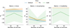 |
Fig. 2 Metrics for age prior distributions for GGL (default), TN, and GGR. The lines and shaded regions depict the mean and standard deviatiom of the five synthetic simulations corresponding to each case. |
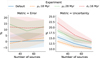 |
Fig. 3 Metrics for shifting and scaling experiments. For comparison purposes, the default configuration without shifting and scaling is also included. The lines and shaded regions depict the mean and standard deviation of the five synthetic simulations corresponding to each case. To save space, the credibility, which is always 100%, is not shown. |
4.2 Sensitivity to shifting and scaling of the a priori age information
We also tested the sensitivity of our prior distributions to shifting and scaling of the prior age information, which represent the most general scenarios in which the literature age estimates can be obtained. These shifting and scaling operations were done by modifying the location (µτ) and scale (στ) hyper-parameters from their nominal values of 23 Myr and 8 Myr, respectively. In the first hyper-parameter experiment, we shifted the nominal location by ±5 Myr and kept the scale at its nominal value. In the second experiment, we kept the location at its nominal value and doubled the scale to a value of 16 Myr.
Figure 3 shows the metrics of the previous experiments as a function of the number of sources. In these shift experiments, the errors have a sign that corresponds to that of the input prior shift, with error values between 10% and 15% for the +5 Myr case and between –3% and 3% for the –5 Myr case. The uncertainties, as expected, reduce with an increasing number of sources, although their values differ. The larger uncertainties correspond to that of the double-scaled experiment and the positive shift, while the smallest to that of the negative shift.
Comparing the results from the different experiments, we observe the following. First, despite the symmetry in the prior shifts, the resulting errors are not symmetric, with the positive shift resulting in a larger bias than the negative shift, which returns almost negligible errors. This behaviour results from the asymmetry introduced via the transformation from expansion rate to ages (see Eq. (1)), in which older ages are more probable than younger ones. Despite this pull of the prior, the resulting estimate remains 100% credible. Second, in the scale experiment, we observe that doubling the prior scale has an impact on the error similar to that of a positive shift, although with slightly larger uncertainty. This behaviour originates from the previously explained asymmetry of the transformation, with older ages being more probable than younger ones. Despite the 12% error, the estimate remains 100% credible in all random realisations.
From the previous experiments, we conclude that whenever the a priori information on the system’s age is scarce, shifting its mode towards younger ages rather than older ones should be preferred. Nonetheless, as these experiments show, a prior shift by up to 20% or a scale degradation by up to 70% of the input age will result in credible age estimates. Despite these comforting results, we encourage the users of the age model, whenever possible, to infer ages with varying prior information and keep in mind that positive errors of 10–15% could be expected.
4.3 Sensitivity to phase-space dispersion
The NYSSs can be found in a variety of phase-space configurations differing from those of the β-Pictoris and Taurus benchmarks. For this reason, we tested the sensitivity of our improved Bayesian age estimator to the phase-space dispersion of stellar systems. To this end, we generated synthetic datasets based on the β-Pictoris template with nominal age and distance, but in which we vary the position dispersion, σXYZ ∈ [0.5,1,5,10,15,20,30,40] pc and the velocity dispersion, σUVW ∈ [0.5,1.0,1.5,2.0]km s −1. Due to the varying phase-space dispersion values, we infer the model parameters using the default dispersion hyper-parameters for the gamma and exponential distributions for the position and velocity dispersions (see Table 2). In addition and for simplicity reasons, we worked with datasets having full radial-velocity coverage.
Figure 4 shows the metrics of the inferred age in the various configurations described above. The figure shows the error and uncertainty metrics as functions of the position dispersion, σXYZ (top panel) and velocity dispersion,σUVW (bottom panel) for systems with 25, 50, and 75 sources. From this figure, we draw the conclusions detailed in the following paragraphs.
Concerning the position dispersion, σXYZ, we observe that the age errors are, on average, smaller than 7% for systems with 50 sources and smaller than 5% for systems with 25 and 75 sources, with these values being uncorrelated with the magnitude of the dispersion up to values of 20 pc. As the dispersion increases beyond the scale length of our default uninformed prior, the errors increase from a few percent up to 5% and 10% for systems with 75 and 25 sources, respectively. The uncertainty shows no correlation with dispersion, and only a decrease with an increasing number of sources, as expected. Finally, the age estimates are 100% credible for all probed values of position dispersion. We notice that the age error in systems with 25 sources is smaller than that of systems with 50 sources. This effect is due to the of the prior, which is centred on the true value and dominates under these low-information content datasets.
Concerning the effects of the velocity dispersion, σUVW, we observe that, similarly to the case of the position dispersion, the errors remain <7% for systems with 50 sources and <3% for those with 75 and 25 sources. On the other hand, contrary to the trend observed in the position dispersion, the age uncertainty increases with increasing velocity dispersion. This effect is expected from the linear velocity model (see Eq. (2) and Lindegren et al. 2000), where the velocity of a star results from the addition of the velocity predicted by the linear velocity field plus a random value drawn from the Gaussian velocity dispersion (first and second terms in Eq. (2), respectively). Therefore, the constraining information provided by the datum of a single star has to be shared by these two terms. As the velocity dispersion increases, the model needs increasing information content to correctly estimate the velocity dispersion due to its exponential prior (see Table 2), which penalises large dispersions. As a result, there is less information available to constrain the linear velocity term, and thus the system’s age is less precise. For this reason, a constraining and fine-tuned velocity dispersion prior will definitively help to increase the precision of the age estimate, as recommended in Sect. 4.1.
From the previous experiments, we draw the following conclusions: first, the age errors of our method are insensitive to the phase-space dispersion (both in positions and velocities) and only mildly so to the number of sources; second, the age uncertainty is sensitive to the velocity dispersion, varying from 10–15% for systems with σUVW ∼ 0.5km s−1 to 19–23% for systems with σUVW ∼ 2.0km s−1. Moreover, we expect that an informed prior in the velocity dispersion will help to further improve the age uncertainty.
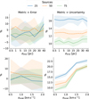 |
Fig. 4 Metrics for phase-space dispersion experiments as a function of the position (top panel) and velocity (bottom panel) dispersion. The lines and shaded regions depict the mean and standard deviation of the five synthetic simulations corresponding to each case of the number of sources. To save space, the credibility, which is always 100%, is not shown. |
4.4 Sensitivity to non-isotropic expansion
The expansion rate of stellar systems is not necessarily isotropic, and this anisotropy may originate from a variety of factors, such as the geometry of the parent molecular cloud, the Galactic potential, or perturbations by nearby stellar systems or molecular clouds. Moreover, as explained in Sect. 3.2.2, the degree of anisotropy varies with the age of the system due to the accumulated effects of the non-symmetric Galactic potential. For all these reasons, we tested the sensitivity of our Bayesian dating method to non-isotropic expansion. To this end, we applied our method with its default and non-isotropic (i.e. Default(κ ∼ StudentT)) configurations to synthetic stellar systems with non-isotropic expansion vectors. As before, we quantified the impact using the error, uncertainty, and credibility metrics.
We generated stellar systems with non-isotropic expansion rates using the β-Pictors template at its nominal distance (see Sect. 2.3). We created two experiments in which the degree of anisotropy was established by varying the three κ components. In the first experiment, which we call mild anisotropy, the three expansion-rate components disagree; we set the X, Y, and Z values so that they correspond (using Eq. (1)) to ages of 18 Myr, 23 Myr, and 28 Myr, respectively. In the second experiment, which we call large anisotropy, two of the entries agree, while the other has negligible expansion. Thus, we set the X, Y, and Z values to correspond with ages of 23 Myr, 23 Myr, and 1Gyr, respectively. This second experiment is intended to test our model in the more realistic scenario whereby the Galactic potential has contracted the system along the Z direction, as in the case of β-Pictoris Mamajek & Bell 2014; Miret-Roig et al. 2020.
Figure 5 shows the metrics obtained after inferring the ages of the two non-isotropic experiments with the default configuration (i.e. Default(µτ = 23, στ = 8)) and the one optimised for non-isotropic expansion (i.e. Default(µτ = 23, στ = 8, κ ~ StudentT), see Sect. 3.2.2). As can be observed from this figure, the default configuration returns negligible 2% errors only in the mild anisotropy case where the value of the κ components disagree by an equivalent of ±5 Myr from the location of the prior. However, in the large anisotropy experiment, we see that the default configuration results in errors varying from 5% for the prior-dominated case with 25 sources to 15% in the data-dominated case with 75 sources. Nonetheless, in spite of the huge difference in age (23 Myr vs. 1 Gyr) between the components of the large anisotropy experiment, our method delivers age estimates that remain 100% credible and with uncertainties between 13% and 17%.
On the other hand, when the age is inferred with our model’s non-isotropic configuration (i.e. Default(µτ = 23, στ = 8, κ ∼ StudentT)), we observe the following improvements. In the mild anisotropy experiment, our model recovers the input age with smaller errors (∼1%) and slightly larger uncertainties than those recovered with the default configuration. In the large anisotropy experiment, we see a considerable reduction in the age errors, which now only reaches 7% in the data-dominated case with 75 sources compared to the 15% of the default configuration. Moreover, the error trend with increasing number of sources is also reduced, resulting in an almost flat behaviour, indicating the stability and robustness of the non-isotropic configuration. The uncertainty in this case is larger than in the default configuration by 2%, but this is a small price to pay considering the reduction in the errors and the large discrepancy in ages from the κ components. Finally, the non-isotropic configuration returns, in both experiments, 100% credibility.
From the previous experiments, we can conclude that although both configurations return 100% credible age estimates, the errors from the non-isotropic configuration are considerably reduced thanks to the robust statistical treatment given by the StudentT distribution. Finally, we recommend users of the age model to infer ages with the non-isotropic configuration whenever they have evidence of anisotropies in the expansionrate components. Nonetheless, biases of up to 10% should be expected in the mean age determinations.
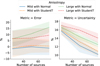 |
Fig. 5 Metrics for non-isotropic expansion experiments. The lines and shaded regions depict the mean and standard deviation of the five synthetic simulations corresponding to each case. To save space, the credibility, which is always 100%, is not shown. |
5 Validation
In this section, we present the validation of our new Bayesian expansion-rate method (Sect. 3) with its default configuration of prior distributions and hyper-parameter values (see Sect. 4; with the informed hyper-parameters for phase-space dispersion using values of Table 1) evaluated on the grid of synthetic systems presented in Sect. 2. First, we present the validation on synthetic stellar associations, and then we finish with the synthetic starforming regions.
5.1 Performance on stellar associations
Figure 6 shows the metrics (as columns) of the Bayesian age estimator as a function of distance colour-coded with the number of a system's sources and grouped in three ages (as rows). The line style shows the fraction of observed radial velocities. At first glance, the errors are for all cases contained within ±10%, the uncertainties are below 20%, and the credibility is always 100%. The overall good values of these metrics over the entire applicability domain shows the excellent properties of our improved expansion-rate dating method.
Concerning errors, we observe that they increase with distance, particularly for datasets with low information content (i.e. those with 25 sources and 25% of observed radial velocities). At the age of 10 Myr, there is no clear difference in the errors incurred in datasets with systems of 25–75 sources, although the errors slightly increase with distance. However, as age increases, there is a wider spread in age error that tends to be on the positive side, with ages overestimated by 5–10%.
Concerning the uncertainty, we observe an overall pattern whereby its value increases with increasing distance and decreases with an increasing number of sources and the fraction of observed radial velocities. Moreover, in the low informationcontent datasets, that is those with 25 sources, we observe a larger dispersion in the metric values compared to those of datasets containing 75 sources. The previous result highlights the importance of compiling membership lists with the largest number of system members, even when they lack radial velocities. Indeed, our results show that doubling the number of sources, even at the cost of halving the fraction of observed radial velocities, provides better constraints to the system’s age than those obtained in datasets with fully observed radial velocities but with half the number of sources.
Concerning credibility, our results show that the Bayesian age estimator provides 100% credible ages in all tested conditions. This high-quality metric results from properly estimated uncertainties and low errors.
In summary, the series of experiments conducted on synthetic stellar associations show that the Bayesian age estimator provides credible ages over its entire applicability domain. Moreover, its age estimates have errors of <10% and uncertainties of <20%.
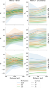 |
Fig. 6 Age metrics of synthetic associations as a function of distance, grouped by age (rows) and colour-coded by number of sources; line style shows the fraction of observed radial velocities. The lines and shaded regions depict the mean and standard deviation of the five synthetic simulations corresponding to each case. To save space, the credibility, which is always 100%, is not shown. |
5.2 Performance on star-forming regions
We applied our Bayesian expansion-rate dating method to the series of synthetic star-forming regions presented in Sect. 2. When applying our method to these datasets, we notice that the default Kalkayotl configuration for the NUTS sampling algorithm faced convergence issues. These issues resulted from both the lack of flexibility of the linear velocity model (see Sect. 3.3 of Olivares et al. 2025), upon which the Bayesian age estimator is constructed, and the phase-space compactness of the synthetic star-forming regions (see Sect. 2.3). To overcome these issues, we increased the number of NUTS sampling chains from two to four and discarded those with divergences, but we always ensured that at least two chains had converged. The metrics of the ages thus inferred are shown in Fig. 7, from which we draw the following conclusions.
Concerning errors, we observe that these vary mostly with age, and their dispersion is reduced by increasing distance and lowering the number of sources. These last two effects are the consequence of the prior, which governs under low informationcontent datasets. The error dispersion reaches its maximum at the closest distance and youngest age, where it varies from 0% to 80%. As the age increases, the error dispersion is reduced to a maximum of 50% at 5 Myr and 35% at 7 Myr.
Concerning uncertainties, we observe that these decrease with age and increase with distance, as expected. At 3 Myr, uncertainties vary between 50% and 80%; at 5 Myr, they vary between 45% and 60%; and, at 7 Myr, they vary between 37% and 47%.
Despite the large errors, the credibility of our age estimates remains at 100%. Thus, in summary, our analysis of synthetic star-forming regions indicates that our Bayesian age estimator demonstrates poorer performance when applied to star-forming regions compared to its results on stellar associations. Therefore, we advise caution when applying our method to the nearest and youngest star-forming regions, where large errors are expected. Moreover, we advise always reporting the 95% credible interval, which, on average, will cover the true age value of the stellar system. Nonetheless, future work will be needed to improve the flexibility of the linear-velocity field model and thus reduce the errors of the Bayesian expansion-rate dating method at the lower frontier of its applicability domain.
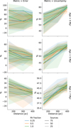 |
Fig. 7 Age metrics of synthetic star-forming regions. Captions are as in Fig. 6. To save space, the credibility, which is always 100%, is not shown. |
6 Discussion
As we validated our method, we can now discuss its advantages with respect to the frequentist approach and the possible caveats inherent to its Bayesian origin. Finally, we also discuss some possible future improvements.
6.1 Bayesian versus frequentist age estimators
In this section, we used the set of synthetic stellar associations (see Sect. 2, Table 1, and Sect. 5.1) to estimate ages with the classical and robust frequentist age estimators (see Sect. 3.1). In this case, we increased the number of synthetic random simulations from five to ten. In these synthetic datasets, the data were first transformed to the physical space of positions and velocities, which implies discarding sources with missing radial velocities, and then the expansion rate components were independently estimated through a robust, linear model regression in which parameter inference was done with the random sample consensus algorithm (Fischler & Bolles 1981) implemented in Scikit-learn (Pedregosa et al. 2011). Then, ages were estimated through weighted means as explained in Sect. 3.1. We then compared these frequentist ages to our Bayesian ones from Sect. 5.1 and discuss their differences based on the value of the error, uncertainty, and credibility metrics.
Figures 8 and 9 show the error, uncertainty, and credibility metrics of the classical and robust frequentist age estimators, respectively. To simplify the comparison, the layout and captions in these figures correspond to those of the Bayesian estimator shown in Fig. 6. From the previous figures, we draw the conclusions detailed in the following paragraphs.
Concerning the classical frequentist estimator (see Fig. 8), we observe that its errors vary with age, distance, number of sources, and fraction of observed radial velocities. We now describe its variation at each age value.
At the youngest age of 10 Myr, the errors increase with a decreasing fraction of observed radial velocities, varying from <±2.5% for 1.0, <±5% for 0.50, and <±10% for 0.25. At the latter value, the ages are overestimated by 10% at the longest distance of 150 pc and underestimated by 10% at the shortest distance of 50 pc. Nonetheless, in all cases, the errors decrease with increasing number of sources, as expected. The uncertainties are also reduced with an increasing number of sources and increasing fraction of observed radial velocities, with values varying from 40% at the farthest away and least populous systems to –10% at the closest and most populated ones. The credibility increases with an increasing fraction of observed radial velocities, varying from 80 –100% at 0.25 to 90 –100% at 1.0. The low credibility in the closest 50 pc systems results from underestimated uncertainties.
At 20 Myr, we observe a degradation of the metrics’ quality, particularly at the low information-content datasets with a distance of 150 pc, 25 sources, and 0.25 fraction of observed radial velocities, where the error reaches values of –200%, the uncertainty is larger than 75%, and the credibility is lower than 50%. As the fraction of observed radial velocity increases from 0.25 to 0.5 and 1.0, the errors are reduced to values between 0 and –15%, –10%, and –5%, respectively. Similarly, the uncertainties improve with decreasing distance and increasing fraction of observed radial velocities and number of sources. These uncertainties vary between 30% and 120% for systems with 25 sources and are reduced to 20–40% for systems with 75 sources. The credibility of systems with 25 sources is also smaller than in the 10 Myr case, with values of 40–50%, 70%–90%, and 90–100% for fractions of observed radial velocities of 0.25, 0.50, and 1.0, respectively. These credibilities increase with increasing number of sources and reach 100% in systems with 75 sources, except at the farthest distance.
At 40 Myr, the degradation of the metrics indicates unreliable age estimates. The errors vary from ±200% to ±50% for fractions of observed radial velocities of 0.25 and 1.0, respectively; there is only a mild improvement with an increasing number of sources in the latter case. The uncertainties have erratic behaviours varying from 100% to 500% and no observable improvement with an increasing number of sources nor an increasing fraction of observed radial velocities. As a consequence of these large errors and erratic uncertainties, the credibilities take values of 10–60%, 20–60%, and 20–60% for fractions of observed radial velocities of 0.25, 0.50, and 1.0, respectively.
We notice that the quality of the metrics decreases with increasing age as a result of both the expansion velocity being inversely proportional to the system’s age and the uncertainties of the observables remaining within the limits of the Gaia properties. Thus, an older true age of the system implies a smaller expansion velocity and lower SNR of the expansion components. As a consequence, as age increases, the frequentist age estimate is governed by errors. Concerning the robust frequentist estimator (see Fig. 9), we observe that its behaviour is similar to the classical one, although with smaller errors and improved uncertainties, which nonetheless result in reduced credibility.
In the 10 Myr case, the errors mildly improve with the number of sources and decrease with increasing fraction of observed radial velocities. For the 0.25, 0.50, and 1.0 values of the latter, the errors take values of ±10%, ±7%, and ±5%, respectively. Similarly, the uncertainties improve mostly with an increasing fraction of observed radial velocities, varying from 10–25% at 0.25, 10–18% at 0.50, and 9–16% at 1.0. With respect to credibility, it improves with increasing fractions of observed radial velocities and number of sources, taking values of 50–100%, 80– 100%, and 90–100% at fractions of observed radial velocities of 0.25, 0.5, and 1.0, respectively.
At 20 Myr, the three metrics are degraded with respect to the 10 Myr case, with now larger errors that underestimate the age in the majority of cases, and uncertainties and credibilities that mildly improve with increasing fraction of observed radial velocities and number of system sources. Surprisingly, the ages are underestimated by 15–35% in systems with 25 sources, and the errors are only reduced to ≲|10|% in systems with 75 sources and fully observed radial velocities. Furthermore, the uncertainties increase with an increasing number of sources, which contradicts the expectations and the results of the classical estimator. Observing the low-credibility values in systems with 25 sources, we conclude that the uncertainty’s unexpected behaviour results from underestimated values in poorly populated systems. Indeed, when the number of sources increases, the uncertainties increase, and the credibility increases as well, but it only reaches values between 60% and 80%.
The 40 Myr case is by far the worst, with highly underestimated ages and uncertainties, resulting in credibilities that are never better than 30%. Moreover, in systems located at 150 pc, there is only one out of ten simulations for systems with 25 sources and a fraction of 0.25 of observed radial velocities in which the expansion-rate component reaches the requested S/N>3. Similarly, at 100 pc, only one out of the ten random simulations of systems with fully observed radial velocities fulfil the SNR criterion. Furthermore, if the SNR criterion were increased, it would further reduce the maximum distance at which the robust estimator returns a value.
Comparing the two frequentist age estimators, we conclude that both are valid for systems with ages up to 10 Myr. Of the two estimators, the classical one returns high credibility values, despite the fraction of observed radial velocities, whereas the robust one only does it for systems with a large fraction of observed radial velocities. From this comparison, we also conclude that discarding one of the expansion-rate components, as is typically done with the Z component (e.g. Mamajek & Bell 2014), will effectively act as the robust estimator and result in an underestimated uncertainty and, as a consequence, low credibility.
Comparing the metrics of the frequentist age estimators with those of the Bayesian one, we observe that the latter outperforms the former in the following aspects. First, its credibility is 100% with 0 dispersion for all ages and cases, meaning that the true age value is always contained within the 95% HDI, whereas for the frequentist estimators this only occurs at the youngest ages with fully observed radial velocities. Second, contrary to the robust frequentist estimator and the classical one at 40 Myr, the Bayesian estimator has uncertainties that always behave as expected, with decreasing values for an increasing number of sources. Moreover, the uncertainties of the Bayesian estimator show small changes of ∼5% with varying distances, while those of the frequentist estimators vary greatly with age and distance, particularly at old ages. Third, the Bayesian uncertainties are, for all cases, ≲20%, which only occurs in the frequentist estimators for 10 Myr and fractions of observed radial velocities >0.5. Fourth, the errors of the Bayesian estimator are always smaller than those of the frequentist estimators, and they are only similar to the latter in the 10 Myr case.
The aforementioned reasons allow us to conclude that, within the applicability domain of our method, our Bayesian age estimator outperforms the frequentist ones providing smaller errors, smaller uncertainties, and 100% credibility. The only metric in which the frequentist estimators beat our Bayesian one is the computation time, where the former takes minutes and the latter takes hours.
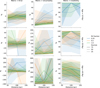 |
Fig. 8 Metrics of classical frequentist age estimator applied to datasets of synthetic associations. The lines and shaded regions depict the mean and standard deviation of the ten synthetic simulations corresponding to each case. |
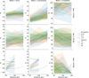 |
Fig. 9 Metrics of robust frequentist age estimator applied to datasets of synthetic associations. Captions as in Fig. 8. |
6.2 Caveats of the Bayesian approach
Although the Bayesian age estimator outperforms its frequentist counterparts, it is not free of caveats and its underlying assumptions are not free of critics. The interested reader will find, in Appendix A, the list of our method’s assumptions together with some basic criticisms of them. Furthermore, as analysed and discussed in Sect. 4, the most important source of bias in our method is the a priori information embedded in the age prior, particularly when this information is biased towards older ages (see Sect. 4.2). However, in real-case scenarios where the true system’s age is not known, it is difficult to know beforehand if the a priori information is biased or not. Thus, in the following, we outline some recommendations for inspecting the prior and minimising its impact on the age’s posterior distribution.
First, it is fundamental to inspect the posterior distribution and compare it with the prior. Ideally, the prior should provide non-negligible probability in intervals where the posterior is not negligible. Moreover, the posterior should shrink with respect to the prior, with the extent of this shrinking being proportional to the information content of the dataset. To help with this posterior inspection, Kalkayotl provides, as part of its standard output, a file with figures in which the prior and posterior distributions of each model parameter are compared with each other. Figure 10 shows an example of this type of figure in which the upper left and upper right panels show kernel density estimates obtained from samples of the prior and posterior distributions, respectively, and the lower panel combines the prior and posterior distributions in the same plot. Using these types of figures, the user can gauge the impact that the prior has on the posterior. For example, in Fig. 11, we compare the posterior distributions (solid lines) inferred for the β-Pictoris template (with 25 sources, fully observed radial velocities, and a true age of 23 Myr), based on the following prior distributions (dotted lines): the younger prior (blue lines) with µτ = 10 Myr and στ = 8 Myr, the centred prior (green lines corresponding to Fig. 10) with µτ = 23 Myr and στ = 8 Myr, and the older prior (red lines) with µτ = 40 Myr and στ = 8 Myr. As can be observed, when the true age is barely contained by the prior, as in the case of the younger prior, only 1% of it is above the true age, and, as a consequence, the majority of the posterior (i.e. the 95% HDI goes from 14.2 to 22.9 Myr) does not include the true age. However, it suffices that only 5% of the prior distribution contains the true age, for the 95% HDI of the posterior to also do it, as in the case of the older prior. Thus, it is of paramount importance to criticise the prior in light of the posterior and ensure that the majority of the latter is contained within the former. For example, in Fig. 10 the prior provides nonnegligible probability over the entire interval where the posterior is not negligible, thus ensuring that: (i) the posterior freely moves on the parameter’s space region constrained by the dataset; and (ii) it shrinks with respect to the prior, as observed by the more compact effective domain (i.e. where the probability is not null).
Second, to avoid biasing the posterior with a restrictive prior, we recommend the use of weakly informative prior distributions (e.g. Gelman et al. 2008) in which the researcher deliberately provides the model with a prior distribution that is wider and less informative than the actual a priori information at hand. The weakly informative prior ensures not only better regularisation properties, it also reduces possible posterior biases. In the astrophysical context of age-dating methods, this type of prior is particularly useful given that the a priori information typically comes from other dating techniques, which are known to disagree (e.g. Galindo-Guil et al. 2022; Barrado y Navascués et al. 1999; Stauffer et al. 1995) and underestimate uncertainties. Thus, our recommendation is to relax the a priori information by embedding a prior distribution with an increased scale.
Third, whenever there are some hints of possible posterior bias due to a restricting prior, we recommend running the inference process with shifted or weakly informative (i.e. scaled) prior distributions until the recommendations of the first point are fulfilled. Doing this ensures that possible age biases remain minimal.
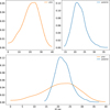 |
Fig. 10 Prior check plot of age parameter (internally called 6D::age, in Myr) computed based on kernel density estimations from samples of the prior (µτ = 23 Myr and στ = 8 Myr) and posterior distributions for the β-Pictoris template with 25 sources and fully observed radial velocities. The top panels independently depict the two distributions, while the bottom one plots them together. |
6.3 Future methodological improvements
From the modelling perspective, we foresee that the method would benefit from the following points: first, constructing the phase-space model on the system’s reference frame (currently, it is only centred on it) and aligning it with the system’s natural axes; second, a more complex phase-space model with second-order velocity field, differential rotation, and differential expansion; third, including proper astrophysical phase-space distributions, as those presented in Olivares et al. (2018), rather than purely statistical ones. Our team is currently working on constructing phase-space models with second-order velocity fields on the natural reference frame of the system, based on nonGaussian multi-variate statistical distributions and mixtures of them.
From the astrophysical perspective, we believe that the nuclear and dynamical dating techniques will benefit from a joint and unified model that simultaneously infers the age of a system using several techniques and in which the systematics among these could be assessed on the basis of robust statistical comparisons. Our team is currently working on a Bayesian hierarchical model that simultaneously infers the age of a system through nuclear and dynamical ages and in which the zero-point offsets between techniques are inferred as free parameters of the model.
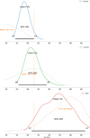 |
Fig. 11 Examples of prior’s influence on the posterior for the case of a realisation of the β-Pictoris template with 25 sources and fully observed radial velocities. The panels show kernel density estimates of the prior (dotted lines) and posterior (solid lines) distributions for the cases in which the prior is younger than (upper panel, µτ = 10 Myr), centred at (mid panel, µτ = 23 Myr), and older than (lower panel, µτ = 40 Myr) the system’s true age of 23 Myr (vertical orange lines). In all cases, the prior dispersion is στ = 8 Myr. The mean and 95% HDI of the posterior are also shown in the black text, while the orange text shows the percentages of the prior distribution that lay below and above the true age. |
7 Conclusions
The testing of current theories of star formation and stellar evolution demands accurate and precise ages of statistically significant samples of stellar systems. Due to their proximity and young ages, the NYSSs have quality data, making them excellent benchmarks to test these theories. Thus, it is of paramount importance to estimate the ages of NYSS with the largest set of properly characterised dating techniques.
In this work, we improved the expansion-rate dating technique with a Bayesian version of it that we make publicly available to the community. This Bayesian expansion-rate method is rooted in the linear velocity field approximation whose parameters are inferred through a robust Bayesian multi-level modelling framework. This Bayesian statistical framework allowed us to incorporate a priori information on the system’s age and establish a robust propagation of correlations and observational uncertainties from the data to the system’s parameters, particularly the age. Using a large corpus of simulations, we proved that our Bayesian version of the expansion-rate method produces age estimates with high-quality metrics (i.e. high credibility and low error) that outperform those of the literature frequentist versions of the method. Nonetheless, our Bayesian age estimator could still be affected by random errors that depend on the system’s properties and prior embedded age information.
Acknowledgements
Acknowledgements.
We thank the anonymous referee for the provided comments and suggestions that greatly improved the quality of this manuscript. JO acknowledge financial support from “Ayudas para contratos postdoctorales de investigación UNED 2021”. “La publicación es parte del proyecto PID2022-142707NA-I00, financiado por MCIN/AEI/10.13039/501100011033/FEDER, UE”. A. Berihuete was also funded by TED2021-130216A-I00 (MCIN/AEI/10.13039/501100011033 and European Union NextGenerationEU/PRTR). We express our gratitude to Anthony Brown, Jos de Bruijne, the Gaia Project Scientist Support Team, and the Gaia Data Processing and Analysis Consortium (DPAC) for providing the PyGaia code. We thank the PyMC team for making publicly available this probabilistic programming language.
Appendix A Assumptions and their criticism
Assumption 1. Young stellar associations are expanding. This assumption neglects possible contraction effects present in the very young stellar systems that may still be collapsing as well as zero-expansion rates in systems that are gravitationally bound.
Assumption 1 can fail in very infant populations and in gravitationally bound systems. In very young systems, its members may still follow the gas dynamics, particularly the infall motion along filaments. Thus, expansion could be present in some spatial directions while contraction in others. Therefore, the age dating method would benefit from kinematic models constructed on the system’s reference frame. In gravitationally bound systems, where expansion is expected to be null, the expansion rate method will simply fail providing an old age. In any case, whenever the total expansion signal is negligible other dating methods should be used instead.
Assumption 2. The observed expansion rate of young stellar associations was imprinted at their birth. This assumption neglects possible time lags between the formation of the association’s stars and the event that originated their expansion.
Assumption 2 could fail if the inferred expansion at the present day resulted from events occurring after the system’s birth time. These events could include: i) supernova explosions, within the system or from a neighbour one, ii) encounters with massive objects, such as other stellar systems or giant molecular clouds, and iii) the gravitational potential removal due to gas expulsion. In all these cases, the expansion rate method would provide a younger age. Although this age would be biased, comparing it with age estimates from other dating techniques could provide valuable information to reconstruct the dynamic history of the system.
Assumption 3. The observed expansion rate of young stellar associations has remained constant since their formation. This assumption neglects possible accelerations or decelerations of the association’s expansion rate due to the Galactic gravitational potential or encounters with other stellar systems and molecular clouds.
Assumption 3 is violated by the presence of the Galactic gravitational potential. However, the accelerations imprinted by the Galactic potential start to distort the original shape of the system only after 40 Myr (Blaauw 1952). Thus, the expansion rate method should remain valid until that age. Future work will be needed to review the validity of this assumption under a variety of realistic conditions.
Assumption 4. The phase-space distribution of a single population is described with a multivariate Gaussian distribution or a linear combination of them. In the latter case, we assume that the Gaussian distributions belong to the same population if and only if their mutual Mahalanobis distances are smaller than 2 (i.e. they are compatible at the 2σ level).
Assumption 4 could fail in systems with complex phasespace morphologies. However, the GMM distribution offers enough flexibility to accommodate non-Gaussian phase-space shapes, as shown by the substructures identified with this model (e.g. Olivares et al. 2023a,b). The expansion rate method could benefit from a GMM in which each component has its independent linear velocity field.
Assumption 5. The astrometry of unresolved binaries corresponds to that of their centre of mass and thus it can be used for the inference of the association parameters as if it were that of a single star. On the contrary, the observed spectroscopic radial velocity of unresolved binaries does not correspond to that of their centre of mass.
Assumption 5 is currently the best we can do to overcome the problems associated with unresolved binaries. In the future, additional information could be added to filter out these sources more efficiently in the data preprocessing steps.
References
- Bailer-Jones, C. A. L. 2015, PASP, 127, 994 [Google Scholar]
- Bailer-Jones, C. A. L. 2023, AJ, 166, 269 [NASA ADS] [CrossRef] [Google Scholar]
- Bailer-Jones, C. A. L., Rybizki, J., Fouesneau, M., Mantelet, G., & Andrae, R. 2018, AJ, 156, 58 [NASA ADS] [CrossRef] [Google Scholar]
- Bailer-Jones, C. A. L., Rybizki, J., Fouesneau, M., Demleitner, M., & Andrae, R. 2021, AJ, 161, 147 [NASA ADS] [CrossRef] [Google Scholar]
- Barrado y Navascués, D., Stauffer, J. R., & Patten, B. M. 1999, ApJ, 522, L53 [Google Scholar]
- Belikov, A. N., Kharchenko, N. V., Piskunov, A. E., Schilbach, E., & Scholz, R. D. 2002, A&A, 387, 117 [NASA ADS] [CrossRef] [EDP Sciences] [Google Scholar]
- Blaauw, A. 1952, Bull. Astron. Inst. Netherlands, 11, 414 [NASA ADS] [Google Scholar]
- Blaauw, A. 1964, ARA&A, 2, 213 [Google Scholar]
- Brown, A. G. A., Dekker, G., & de Zeeuw, P. T. 1997, MNRAS, 285, 479 [NASA ADS] [CrossRef] [Google Scholar]
- Casamiquela, L., Olivares, J., Tarricq, Y., et al. 2022, A&A, 664, A31 [NASA ADS] [CrossRef] [EDP Sciences] [Google Scholar]
- Fischler, M. A., & Bolles, R. C. 1981, Commun. ACM, 24, 381 [CrossRef] [Google Scholar]
- Gagné, J., Mamajek, E. E., Malo, L., et al. 2018, ApJ, 856, 23 [Google Scholar]
- Galindo-Guil, F. J., Barrado, D., Bouy, H., et al. 2022, A&A, 664, A70 [NASA ADS] [CrossRef] [EDP Sciences] [Google Scholar]
- Galli, P. A. B., Loinard, L., Bouy, H., et al. 2019, A&A, 630, A137 [NASA ADS] [CrossRef] [EDP Sciences] [Google Scholar]
- Galli, P. A. B., Miret-Roig, N., Bouy, H., Olivares, J., & Barrado, D. 2023, MNRAS, 520, 6245 [NASA ADS] [CrossRef] [Google Scholar]
- Gelman, A., Carlin, J. B., Stern, H. S., et al. 2014, Bayesian Data Analysis (Boca Raton, FL: Chapman & Hall) [Google Scholar]
- Gelman, A., Jakulin, A., Pittau, M. G., & Su, Y.-S. 2008, Ann. Appl. Statist., 2, 1360 [Google Scholar]
- Hoffman, M. D., & Gelman, A. 2011, arXiv e-prints, [arXiv:1111.4246] [Google Scholar]
- Jeffries, R. D., Jackson, R. J., Wright, N. J., et al. 2023, MNRAS, 523, 802 [NASA ADS] [CrossRef] [Google Scholar]
- Juárez, M. A., & Steel, M. F. J. 2010, J. Business Econ. Statist., 28, 52 [Google Scholar]
- Lee, R. A., Gaidos, E., van Saders, J., Feiden, G. A., & Gagné, J. 2024, MNRAS, submitted [arXiv:2312.15792] [Google Scholar]
- Lindegren, L., Madsen, S., & Dravins, D. 2000, A&A, 356, 1119 [Google Scholar]
- Luhman, K. L. 2022, AJ, 164, 151 [NASA ADS] [CrossRef] [Google Scholar]
- Luhman, K. L. 2023, AJ, 165, 269 [NASA ADS] [CrossRef] [Google Scholar]
- Mamajek, E. E., & Bell, C. P. M. 2014, MNRAS, 445, 2169 [Google Scholar]
- Miret-Roig, N., Galli, P. A. B., Brandner, W., et al. 2020, A&A, 642, A179 [NASA ADS] [CrossRef] [EDP Sciences] [Google Scholar]
- Miret-Roig, N., Galli, P. A. B., Olivares, J., et al. 2022, A&A, 667, A163 [NASA ADS] [CrossRef] [EDP Sciences] [Google Scholar]
- Morton, T. D. 2015, isochrones: Stellar model grid package, Astrophysics Source Code Library, [record ascl:1503.010] [Google Scholar]
- Olivares, J., Moraux, E., Sarro, L. M., et al. 2018, A&A, 612, A70 [NASA ADS] [CrossRef] [EDP Sciences] [Google Scholar]
- Olivares, J., Sarro, L. M., Bouy, H., et al. 2020, A&A, 644, A7 [NASA ADS] [CrossRef] [EDP Sciences] [Google Scholar]
- Olivares, J., Bouy, H., Miret-Roig, N., et al. 2023a, A&A, 671, A1 [NASA ADS] [CrossRef] [EDP Sciences] [Google Scholar]
- Olivares, J., Lodieu, N., Béjar, V. J. S., et al. 2023b, A&A, 675, A28 [NASA ADS] [CrossRef] [EDP Sciences] [Google Scholar]
- Olivares, J., Bouy, H., Dorn-Wallenstein, T. Z., & Berihuete, A. 2025, A&A, 693, A12 [NASA ADS] [CrossRef] [EDP Sciences] [Google Scholar]
- Oriol, A.-P., Virgile, A., Colin, C., et al. 2023, PeerJ Comput. Sci., 9, e1516 [CrossRef] [Google Scholar]
- Pedregosa, F., Varoquaux, G., Gramfort, A., et al. 2011, J. Mach. Learn. Res., 12, 2825 [Google Scholar]
- Ratzenböck, S., Großschedl, J. E., Alves, J., et al. 2023, A&A, 678, A71 [NASA ADS] [CrossRef] [EDP Sciences] [Google Scholar]
- Stacy, E. W. 1962, Ann. Math. Statist., 33, 1187 [CrossRef] [Google Scholar]
- Stauffer, J. R., Liebert, J., & Giampapa, M. 1995, AJ, 109, 298 [NASA ADS] [CrossRef] [Google Scholar]
- von Hippel, T., Jefferys, W. H., Scott, J., et al. 2006, ApJ, 645, 1436 [Google Scholar]
- Wright, N. J., & Mamajek, E. E. 2018, MNRAS, 476, 381 [Google Scholar]
- Wright, N. J., Jeffries, R. D., Jackson, R. J., et al. 2024, MNRAS, 533, 705 [NASA ADS] [CrossRef] [Google Scholar]
- Zari, E., Brown, A. G. A., & de Zeeuw, P. T. 2019, A&A, 628, A123 [NASA ADS] [CrossRef] [EDP Sciences] [Google Scholar]
For the generalised gamma with negative skewness to have the required standard deviation, the input scale must be multiplied by the factor  .
.
All Tables
All Figures
|
Fig. 1 Comparison of our age prior distributions. The hyper-parameters (µτ and στ) were fixed to values that result in a distribution with mode and variance corresponding to those for the β-Pictoris stellar association, 23 ± 8 Myr (Lee et al. 2024). |
| In the text | |
|
Fig. 2 Metrics for age prior distributions for GGL (default), TN, and GGR. The lines and shaded regions depict the mean and standard deviatiom of the five synthetic simulations corresponding to each case. |
| In the text | |
|
Fig. 3 Metrics for shifting and scaling experiments. For comparison purposes, the default configuration without shifting and scaling is also included. The lines and shaded regions depict the mean and standard deviation of the five synthetic simulations corresponding to each case. To save space, the credibility, which is always 100%, is not shown. |
| In the text | |
|
Fig. 4 Metrics for phase-space dispersion experiments as a function of the position (top panel) and velocity (bottom panel) dispersion. The lines and shaded regions depict the mean and standard deviation of the five synthetic simulations corresponding to each case of the number of sources. To save space, the credibility, which is always 100%, is not shown. |
| In the text | |
|
Fig. 5 Metrics for non-isotropic expansion experiments. The lines and shaded regions depict the mean and standard deviation of the five synthetic simulations corresponding to each case. To save space, the credibility, which is always 100%, is not shown. |
| In the text | |
|
Fig. 6 Age metrics of synthetic associations as a function of distance, grouped by age (rows) and colour-coded by number of sources; line style shows the fraction of observed radial velocities. The lines and shaded regions depict the mean and standard deviation of the five synthetic simulations corresponding to each case. To save space, the credibility, which is always 100%, is not shown. |
| In the text | |
|
Fig. 7 Age metrics of synthetic star-forming regions. Captions are as in Fig. 6. To save space, the credibility, which is always 100%, is not shown. |
| In the text | |
|
Fig. 8 Metrics of classical frequentist age estimator applied to datasets of synthetic associations. The lines and shaded regions depict the mean and standard deviation of the ten synthetic simulations corresponding to each case. |
| In the text | |
|
Fig. 9 Metrics of robust frequentist age estimator applied to datasets of synthetic associations. Captions as in Fig. 8. |
| In the text | |
|
Fig. 10 Prior check plot of age parameter (internally called 6D::age, in Myr) computed based on kernel density estimations from samples of the prior (µτ = 23 Myr and στ = 8 Myr) and posterior distributions for the β-Pictoris template with 25 sources and fully observed radial velocities. The top panels independently depict the two distributions, while the bottom one plots them together. |
| In the text | |
|
Fig. 11 Examples of prior’s influence on the posterior for the case of a realisation of the β-Pictoris template with 25 sources and fully observed radial velocities. The panels show kernel density estimates of the prior (dotted lines) and posterior (solid lines) distributions for the cases in which the prior is younger than (upper panel, µτ = 10 Myr), centred at (mid panel, µτ = 23 Myr), and older than (lower panel, µτ = 40 Myr) the system’s true age of 23 Myr (vertical orange lines). In all cases, the prior dispersion is στ = 8 Myr. The mean and 95% HDI of the posterior are also shown in the black text, while the orange text shows the percentages of the prior distribution that lay below and above the true age. |
| In the text | |
Current usage metrics show cumulative count of Article Views (full-text article views including HTML views, PDF and ePub downloads, according to the available data) and Abstracts Views on Vision4Press platform.
Data correspond to usage on the plateform after 2015. The current usage metrics is available 48-96 hours after online publication and is updated daily on week days.
Initial download of the metrics may take a while.