| Issue |
A&A
Volume 700, August 2025
|
|
|---|---|---|
| Article Number | A45 | |
| Number of page(s) | 18 | |
| Section | Planets, planetary systems, and small bodies | |
| DOI | https://doi.org/10.1051/0004-6361/202554303 | |
| Published online | 04 August 2025 | |
A high geometric albedo for LTT9779b points toward a metal-rich atmosphere and silicate clouds
1
Instituto de Estudios Astrofísicos, Facultad de Ingeniería Ciencias, Universidad Diego Portales,
Av. Ejército Libertador 441,
Santiago,
Chile
2
Centro de Excelencia en Astrofísica y Tecnologías Afines (CATA),
Camino El Observatorio 1515,
Las Condes,
Santiago,
Chile
3
Université Côte d’Azur, Observatoire de la Côte d’Azur, CNRS, Laboratoire Lagrange,
France
4
Aix Marseille Univ, CNRS, CNES, LAM,
38 reu Frédérik Joliot-Curie,
13388
Marseille,
France
5
Department of Physics and Astronomy, University of Kansas,
Lawrence,
KS,
USA
6
Instituto de Astronomía, Universidad Católica del Norte,
Angamos 0610,
1270709
Antofagasta,
Chile
7
Instituto de Astrofisica, Departamento de Fisica y Astronomia, Facultad Ciencias Exactas, Universidad Andres Bello,
Fernandez Concha 700,
Las Condes,
Santiago,
Chile
8
Departamento de Astronomía, Universidad de Chile,
Camino el Observatorio 1515,
Las Condes,
Santiago,
Chile
9
Las Campanas Observatory, Carnegie Institution for Science,
Raul Bitrán 1200,
La Serena,
Chile
* Corresponding author: This email address is being protected from spambots. You need JavaScript enabled to view it.
Received:
27
February
2025
Accepted:
12
June
2025
Abstract
Aims. In this work, our aim is to confirm the high albedo of the benchmark ultra-hot Neptune LTT9779b using 20 secondary eclipse measurements of the planet observed with CHEOPS. In addition, we performed a search for variability in the reflected light intensity of the planet as a function of time.
Methods. First, we used the TESS follow-up data of LTT9779b from three sectors (2, 29, and 69) to remodel the transit signature and estimate an updated set of transit and ephemeris parameters, which were directly used in the modeling of the secondary eclipse light curves. This involved a critical noise-treatment algorithm, including sophisticated techniques such as wavelet denoising and Gaussian process (GP) regression, to constrain noise levels from various sources. In addition to using the officially released reduced aperture photometry data from CHEOPS DRP, we also reduced the raw data using an independent PSF photometry pipeline, known as PIPE, to verify the robustness of our analysis. The extracted secondary eclipse light curves were modeled using the PYCHEOPS package, where we detrended the background noise correlated with the spacecraft roll angle, originating from the inhomogeneous and asymmetric shape of the CHEOPS point spread function, using an N-order glint function.
Results. Our independent light curve analyses have resulted in consistent estimations of the eclipse depths, with values of 89.9 ± 13.7 ppm for the DRP analysis and 85.2 ± 13.1 ppm from PIPE, indicating a high degree of statistical agreement. Adopting the DRP value yields a highly constrained geometric albedo of 0.73 ± 0.11. No significant eclipse depth variability is detected down to a level of ∼ 37 ppm.
Conclusions. Our results confirm that LTT9779b exhibits a strikingly high optical albedo, which substantially reduces the internal energy budget of the planet compared to more opaque atmospheres. By modeling our new and precise eclipse measurements, we find that the planet’s atmosphere is likely highly metal-rich, with silicate clouds probably present. Our models find it difficult to explain the high geometric albedo since fitting these high optical bands leads to a decrease in the near-IR planetary emission, well below the current observations. However, we discuss additional physical processes that could circumvent this problem, such as the introduction of strong particle backscattering.
Key words: techniques: photometric / planets and satellites: atmospheres / planets and satellites: gaseous planets
© The Authors 2025
 Open Access article, published by EDP Sciences, under the terms of the Creative Commons Attribution License (https://creativecommons.org/licenses/by/4.0), which permits unrestricted use, distribution, and reproduction in any medium, provided the original work is properly cited.
This article is published in open access under the Subscribe to Open model. This email address is being protected from spambots. You need JavaScript enabled to view it. to support open access publication.
1 Introduction
Observations of optical secondary eclipses of planets can provide a detailed understanding of the reflected light properties of these worlds, and with that comes a more complete picture of the energy budget and atmospheric structure, or surface constituents. Due to the photometric precision requirements necessary to make these occultation measurements possible, the majority of reflected light studies have been performed on hot Jupiters (HJs) since their larger physical size presents a more favorable target for the outgoing photon flux from the host star (e.g., Brandeker et al. 2022; Krenn et al. 2023; Pagano et al. 2024).
Although HJs appear to be excellent targets for optical reflected light studies, some of the first searches for this signature foreshadowed what was to come later when we had even more precise facilities. The lack of any confirmed detections for planets such as Tau Bootis b (Leigh et al. 2003a; Collier-Cameron et al. 2004), HD 75289b (Leigh et al. 2003b), and HD 209458b (Rowe et al. 2008) could place upper limits on the geometric albedo (Ag) in the range of ∼ 0.15–0.40. Subsequent studies were able to show that HJs in general are very dark planets, having Ag values of ∼ 0.1 (Esteves et al. 2015), meaning they do not reflect a large fraction of the incident stellar flux falling on their upper atmospheres.
The albedo of a planet’s atmosphere is set by the competition between the absorption and reflection of stellar light. Given the high temperatures of hot and ultra-hot Jupiters, numerous absorbers can be in the vapor phase: titanium and vanadium oxide for the hottest planets, sodium and potassium for the cooler ones (Fortney et al. 2008). In HJs, Rayleigh scattering by the gas is usually much smaller than the absorption by these optical absorbers (see class IV planets by Sudarsky et al. 2000). Therefore, these planets could have a high albedo only if condensed particles reflect back a significant portion of the light. The most likely species to make a thick enough cloud cover to affect the albedo are silicate clouds. As shown by the class V planets of Sudarsky et al. (2000), the inclusion of such a thick silicate cloud would raise the albedo of planetary atmospheres to high values.
However, Jupiter-sized planets hotter than 2000 K, also known as ultra-hot Jupiters, are unlikely to form these clouds on their dayside. These planets have a strong thermal inversion (predicted by Fortney et al. 2008 and recently unambiguously observed by JWST in Coulombe et al. 2023), driven by the optical absorption of the light by TiO and VO in the upper atmospheres. Their dayside atmospheres therefore become hot enough to thermally dissociate molecules (Parmentier et al. 2018), and are clearly too hot to host any type of clouds on the dayside.
At the other end of the planetary spectrum, small planets that physically present less favorable targets have still been studied in some detail, in particular the super-Earth population. Although still a relatively small statistical sample, discoveries from the Kepler mission (Borucki et al. 2010) provided the first look at the reflective properties of these planets, and showed a pattern similar to the HJs: in general super-Earths and sub-Neptunes can be as opaque as HJs, having Ag values of 0.11 ± 0.06 and 0.05 ± 0.04 respectively, whereas the super-Neptunes are a little more reflective, with Ag values of ∼ 0.23 ± 0.11 (Sheets & Deming 2017). As can be seen by the significantly larger uncertainty on the super-Neptune albedo mean value, the sample used was small, only containing 12 systems, since they were validated to have false positive probabilities of less than 1%, even though they were not fully confirmed as genuine planets at the time of publication. However, these results hint that super-Neptunes may present a unique group of worlds that showcase atmospheric structures more susceptible to reflectivity, possibly due to the presence of a high atmospheric metallicity and so many host structures, for example, high-altitude silicate cloud decks.
In 2023, the first optical secondary eclipse of a confirmed ultra-hot Neptune (UHN), which is also a super-Neptune planet with a radius of ∼ 4.5 R⊕, was published (Hoyer et al. 2023, hereafter H23). Using the CHaracterising ExOPlanets Satellite (CHEOPS; Benz et al. 2021), H23 observed ten optical eclipses of LTT9779b, arriving at a mean eclipse depth of 115 ± 24 ppm in the CHEOPS bandpass, which gives an Ag of 0.80 ± 0.17, similar to that of Venus in our Solar System. Such a high albedo points toward the presence of a highly reflective silicate cloud layer in the upper atmosphere. The team further showed that the presence of these refractory clouds at such a high equilibrium temperature (∼ 2000 K; Jenkins et al. 2020) is possible if the atmosphere is extremely metal-rich and saturated in metals. Observations from Spitzer, JWST, WINERED, and ESPRESSO all point toward a planet with a metallicity greater than 20× solar (Crossfield et al. 2020; Radica et al. 2024; Vissapragada et al. 2024; Ramírez Reyes et al. 2025), and the CHEOPS data also indicated the lower limit was 400 × solar. On the other hand, while Edwards et al. (2023) and the recently published Coulombe et al. (2025) reported lower retrieved metallicities from HST transmission and JWST emission spectra, respectively, both studies acknowledge limitations arising from the restricted wavelength coverage, which hinders the accurate detection of carbon-bearing molecules.
One of the interesting issues H23 faced when trying to model the spectral energy distribution (SED) of the planet with 1D radiative transfer models was capturing the strong CHEOPS optical eclipse depth, while also accurately fitting the large discrepancy between the Spitzer 3.6 and 4.5 μm bands (see Dragomir et al. 2020, who suggested the presence of CO, CO2, and/or clouds to explain this observation). Various atmospheric metallicities and heat redistribution factors were tested in order to best fit the data; it was found that the atmosphere is likely super metal-rich, and there is only intermediate heat redistribution around the planet. The Spitzer phase curve analysis presented in Crossfield et al. (2020) also indicated an inefficient heat redistribution around the atmosphere, along with the possible metal-rich atmosphere mentioned above.
With such a high atmospheric metallicity being suggested for this planet, attempts to constrain the atmospheric metals further using space-based low- to medium-resolution spectrophotometry with JWST and/or ground-based high-resolution spectroscopy using ESPRESSO, for example, have been made. Radica et al. (2024) have found >5 σ detection of suppressed spectral features in transmission using NIRISS/SOSS on board JWST; however, after exploring various water- and methane-dominated atmospheres, they realized that a number of different scenarios can fit the data equally well, and that they are particularly dependent on the actual atmospheric metallicity. Ramírez Reyes et al. (2025) also studied the planet in transmission from the ground using high-resolution spectroscopy with ESPRESSO; they find no clear detections of single-line elements, for example sodium, nor other elements, for example TiO, using the cross-correlation technique. However, this work again pointed toward a super metal-rich atmosphere for LTT9779b since increasing the atmospheric metallicity decreases the scale height, rendering absorption signatures too weak to detect with the current data. Therefore, taking all these previous efforts together, there is a clear line of evidence that suggests LTT9779b hosts a large rocky core surrounded by a compact but super metal-rich atmosphere. Further constraining the structure and atmospheric chemistry of this atmosphere is a high priority to better understand the formation and evolutionary mechanisms that occur for extreme planets deeply embedded in the Neptune desert.
This paper is set out to discuss in detail the results from observing an additional ten CHEOPS secondary eclipses of LTT9779b beyond those already examined in the earlier work of H23. With these 20 occultations, we can provide even stricter constraints on the geometric albedo of this planet, along with providing a more accurate modeling framework to understand the atmospheric structure. In Sect. 2 we discuss the photometric time series observations from the Transiting Exoplanet Survey Satellite (TESS; Ricker et al. 2015) and from CHEOPS. In Sect. 3 we discuss in detail the processing and modeling of these light curves. In Sect. 4 we detail our modeling efforts to fit these new optical eclipse depths, in addition to the already published near-infrared (NIR) eclipse depths. Finally, in Sect. 5 we contextualize our results within the broader picture of planet formation and evolution, and summarize our findings.
2 Observations
2.1 TESS transit observations
TESS observed LTT9779 during sectors 2, 29, and 69, the corresponding sector mid-points being in September 2018, September 2020, and September 2023, respectively. The previous studies that reported the transit properties of LTT9779b (e.g. Jenkins et al. 2020) used the TESS observations only from sector 2. Since a precise estimation of the transit parameters, including the ephemeris, is extremely important for precise modeling of secondary eclipse observations, we decided to model all the transit light curves observed from all three TESS sectors for an updated estimation of the parameters.
We used the Barbara A. Mikulski Archive for Space Telescopes (MAST)1 to download the publicly available TESS data for LTT9779 corresponding to the mentioned sectors. For all three sectors, the standard 120s cadence PDCSAP light curves, processed using the Science Processing Operations Center (SPOC, Jenkins et al. 2016; Caldwell et al. 2020) pipeline, were available, which we adopted for our analyses. We identified 87 full transit observations from these light curve data. More details on the analyses and modeling of the light curves are given in Section 3.1.
Details of the CHEOPS observations.
2.2 CHEOPS secondary eclipse observations
We observed 20 secondary eclipse events LTT9779b from CHEOPS (PI: James Jenkins), the first 10 of which were obtained during September-October 2020 (also see Hoyer et al. 2023), followed by 10 further observations during August-October 2022. The data corresponding to these observations are now publicly available at the CHEOPS archive2. Table 1 lists the details of these observations. The epochs are with respect to the first transit of LTT9779b detected by TESS. The table also provides the percentage of the whole secondary eclipse events covered by the CHEOPS observations, calculated using the orbital ephemeris and transit duration estimated from the transit modeling of the TESS light curves in this work (details in Section 3.1). The interruptions in CHEOPS observations are caused by high levels of stray light (SL) and South Atlantic Anomaly (SAA) crossings (Benz et al. 2021). The detail of the analyses and modeling of the CHEOPS data is described in Section 3.2.
3 Analyses and modeling
3.1 TESS light curves
The long TESS light curves were sliced, each part containing the full-transit observations, along with significant baselines (at least three times the transit duration) on either side of the transits, to obtain 87 transit light curves. The large-scale variations in these transit light curves, originating from the long-term variation in the stellar flux and instrumental factors, were reduced using a baseline correction method (e.g. Saha 2022, 2023), where the out-of-transit sections of the light curves were modeled using a first-order and a second-order polynomial, and the best-fit models with the least Bayesian information criterion (BIC, e.g. Neath & Cavanaugh 2012) were subtracted from the entire light curves.
To reduce the time-uncorrelated fluctuations in the light curves, the wavelet denoising (Donoho & Johnstone 1994; Quan Pan et al. 1999; Luo & Zhang 2012; Saha et al. 2021; Saha & Sengupta 2021) technique was used. This is particularly useful for TESS data, where the signals are more susceptible to photometric contamination from background sources. Wavelet denoising does not affect the high-frequency terms (such as ingress or egress of a transit) in the signals, unlike other smoothing techniques such as binning or Gaussian moving averages. Instead, it selectively targets lower-amplitude noise components in the light curves, which are distinct from the large transit signatures, thereby providing the flexibility to enhance photometric precision without distorting them (e.g. Saha & Sengupta 2021). Our implementation of wavelet denoising is similar to Saha (2024, 2025), where the Symlet family of wavelets (Daubechies 1988), which are the least asymmetric modified versions of the Daubechies wavelets (Daubechies 1992; Rowe & Abbott 1995), were used. For the discrete wavelet transforms (DWTs), the PyWavelets (Lee et al. 2019) package was used. We used a level-1 wavelet denoising in order to avoid oversmoothing, along with the implementation of the universal thresholding law (Donoho & Johnstone 1994).
In order to reduce the effect of the time-correlated noise components in the transit light curves, which originate from the small-scale variability and pulsations of the host star, as well as instrumental effects, we modeled the time-correlated noise using the Gaussian process (GP) regression method (Rasmussen & Williams 2006; Johnson et al. 2015; Pereira et al. 2019; Saha et al. 2021; Saha & Sengupta 2021), while simultaneously modeling the transit signatures in the light curves. We used a procedure similar to that in Saha (2024, 2025) for the GP regression, which uses the Matern class covariance function with v = 3/2, with two free parameters, i.e., the signal standard deviation and characteristic timescale. The analytical transit formalism by Mandel & Agol (2002) was used for the transit modeling. The simultaneous transit modeling with GP regression was performed by the Markov chain Monte Carlo (MCMC) sampling technique, with the implementation of the Hastings-Metropolis algorithm (Hastings 1970). Figure 1 shows a representative subset of the modeled transit light curves, with the rest shown in Figure A.3 in the Appendix. The estimated mid-transit times from the transit modeling were used to estimate the linear orbital ephemeris. Combined with the stellar and radial velocity parameters from Jenkins et al. (2020), other derivable parameters for the system were estimated. All the estimated and derived parameters are listed in Table 2.
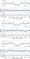 |
Fig. 1 Observed and best-fit model light curves corresponding to the first transit observed from each TESS sector. For each transit, the top panel shows the unprocessed light curve (light blue), the light curve after wavelet denoising (blue), and the best-fit transit model (brown); the middle panel shows the residual flux before GP regression (blue), and the mean (green) and 1 σ interval (light blue) of the best-fit GP regression model; and the bottom panel shows the final mean residual flux (blue). The mean residual flux corresponds to the residual flux considering the mean of the best-fit GP regression model. |
Estimated physical properties for LTT9779b from the transit modeling of TESS light curves.
3.2 CHEOPS secondary eclipse observations
The CHEOPS data products downloadable from the official CHEOPS archive consist of raw data, as well as time series data reduced using the official Data Reduction Pipeline (DRP, Hoyer et al. 2020). The time series data are available for aperture photometry performed using different aperture sizes, ranging from 15 to 40 pixels. We examined the light curves generated from these different aperture sizes and found the data corresponding to the aperture size of 24 pixels to be the best in terms of light curve dispersion for the majority of the cases. Since the secondary eclipse depths are expected to be small when compared with various sources of contamination possible in the photometric data, it is prudent to use a second independent data reduction, so that the analyses and results can be cross-verified. Thus, we also performed an independent reduction of the raw CHEOPS data using the PSF Imagette Photometric Extraction (PIPE, Brandeker et al. 2024) package. As the name suggests, PIPE uses the point spread function (PSF) photometry method and was successfully adopted by several previous studies (e.g., Serrano et al. 2022; Singh et al. 2024).
For the analyses and modeling of the secondary eclipse light curves, we used the PYCHEOPS (Maxted et al. 2022) package, which was exclusively developed for the analyses of CHEOPS data. First, we removed the large outliers in the light curves resulting from cosmic ray hits. The inhomogeneous and asymmetric shape of the CHEOPS PSF (Benz et al. 2021) adds a roll-angle-dependent variation in the background flux to the light curves. The presence of two close-by stars with G = 19 and G = 15 at respective distances to the source of 19′′ and 21′′ (see Hoyer et al. 2023) contributed primarily to this variation for our secondary eclipse light curves. We used a glint function to simultaneously model this background variation, correlated with the roll-angle, while modeling the secondary eclipses. We used the glint function with a fixed number of splines (Ns = 32) and an independent glint scale parameter (see Figure 2).
The modeling of the secondary eclipses was performed using the MCMC sampling technique, where we used the updated transit parameters estimated from our TESS transit light curve analyses, including the more precise ephemeris, as fixed parameters, keeping the eclipse depths as the independent variables. The depths of the secondary eclipses from each epoch were estimated independently for both sets of light curves reduced using the DRP and PIPE. We found that the detrended light curves from both DRP and PIPE outputs are in statistical agreement with each other (see Figure 3, and Figure A.1 in the Appendix). This helps cross-verify our data reduction and pre-processing steps. The estimated depths of all the secondary eclipses from the light curves reduced by both the DRP and PIPE, along with the calculated mean depths, are given in Table 3. Figure 4 is a graphical representation of these tables, where it can be seen that the estimated depths from the light curves reduced by the DRP and PIPE are in statistical agreement with each other. We also modeled all the light curves simultaneously with a single eclipse depth, which resulted in larger residual trends in the fitted light curves. This suggests a dynamically varying nature for these eclipses, with some eclipses dropping below our detection threshold and others well above. However, we were not able to confirm the atmosphere’s variable nature statistically because of limited S/N and large systematics in our observed data.
We estimated mean eclipse depths from the DRP and PIPE light curves to be 89.85 ± 13.68 ppm and 85.2 ± 13.05 ppm, respectively. Based on these values, we calculated the corresponding geometric albedos of LTT9779b to be 0.73 ± 0.11 and 0.70 ± 0.11, from the DRP and PIPE reductions, respectively (also see Figure 5). We note that we report arithmetic means here; if we performed a weighted mean, we would arrive at a lower eclipse depth (e.g., 58.1 ± 10.6 ppm from DRP), which remains in statistical agreement with the nonweighted value. However, by weighting, we are heavily biasing toward the nondetections (those with depths below ∼ 55 ppm), as these appear to have more precise measurements due to the fact that the uncertainty spread cannot be negative (essentially they all have ∼ 100% uncertainties), setting our detection limit. Therefore, we chose to conservatively take the arithmetic mean, which is in excellent statistical agreement with H23, but with substantially improved statistical precision. The revised eclipse depth is also consistent with Radica et al. (2025), who noted that the H23 value was somewhat larger than predicted by their models. In addition, a very recent study using JWST/NIRISS phase curve observations (Coulombe et al. 2025) suggests a varying albedo of 0.41 ± 10 to 0.79 ± 0.15 from the eastern to the western dayside of LTT9779b. While the upper limits from these results are in good statistical agreement with our estimated values, they also point toward a dynamically changing atmosphere of this planet, as we had suggested in H23 and allude to here.
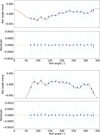 |
Fig. 2 Trends in the background flux variations with respect to the roll-angle for the CHEOPS observation corresponding to epoch 1889, from the light curves reduced by the DRP (top) and PIPE (bottom). The light blue points show individual observations (without uncertainties), and the blue points show data binned over 15° intervals. It is worth noting that the trend of variation is different between the light curves reduced using the DRP and PIPE, since PIPE has a different sensitivity to background stars that contaminate the photometric apertures in the DRP outputs. |
Estimated secondary eclipse depths from the light curves reduced by DRP and PIPE.
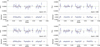 |
Fig. 3 Detrended individual (light blue, without uncertainties) and binned (blue, binned over 7.2 min intervals) secondary eclipse light curves corresponding to epochs 971 and 1889, reduced by using the DRP (top) and PIPE (bottom). The best-fit transit models are shown as brown lines (the green portions show the disruptions in the light curves), and the residuals from the best-fit models in the bottom panels. The light curves reduced by the DRP and PIPE are in statistical agreement with each other. |
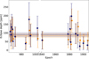 |
Fig. 4 Secondary eclipse depths estimated for each individual epoch from the light curves reduced by the DRP (blue) and PIPE (orange, with a slight offset along the x-axis for visibility), along with the calculated mean secondary eclipse depths (blue and orange dotted lines for the light curves reduced by DRP and PIPE respectively; the shaded regions show the uncertainties). We note that the eclipse depths estimated from the two sets of light curve data reduced by independent pipelines (i.e., DRP and PIPE) are in close statistical agreement with each other. |
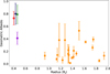 |
Fig. 5 Geometric albedo vs. radius plot for LTT9779b estimated from this work (DRP, red), from Hoyer et al. 2023 (blue), and from Coulombe et al. 2025 (western dayside in green and eastern dayside in violet) also showing the known well-constrained geometric albedos of other hot and ultra-hot Jupiters from the literature (orange). |
4 Interpretation
4.1 Model setup
In order to interpret our measured eclipse depth, we used the radiative-convective-chemical equilibrium code scCHIMERA (Line et al. 2021; Wiser et al. 2024). The code solves for the radiative-convective state of the atmosphere while assuming that chemical equilibrium is maintained at all times. The chemical equilibrium is calculated with the CEA Gibbs free energy minimization code. The code takes into account both titanium-based clouds and silicate clouds (MgSiO3). However, we find that only the silicate clouds have a high enough opacity to affect the albedo of the planet. When a given species condenses out of the atmosphere, we assume that it is not locally available to react chemically with the atmosphere. We further assume that all layers above the condensation level have an abundance of the condensed species that are set by the partial pressure of the species at the cloud formation level (vertical rainout approximation).
When chemical equilibrium predicts cloud condensation, we solve the vertical structure of the cloud using the formalism from (Ackerman & Marley 2001). This formalism assumes a balance between the settling rate of the particles (and thus their size) and the vertical mixing.
Metallicity is changed in the atmosphere by first multiplying all elemental abundances of species other than H and He by the metallicity factor, and then normalizing all elements so that the sum of their volume mixing ratios equals 1. This approach ensures that the ratio of all elements remains solar, but that all are enriched compared to hydrogen.
We have already shown in Hoyer et al. (2023) that to obtain a high albedo through cloud formation for LTT9779b, a high metallicity was required, but also that the exact metallicity was degenerate with the heat transport efficiency. We therefore updated the scCHIMERA models to better model the reflected light of LTT9779b. When solving for the equilibrium thermal structure of the planet’s dayside, we adjust the incoming irradiation to take into account the fact that some energy is transported toward the dayside. In terms of modeling, this is accomplished by modulating the received stellar flux by a redistribution factor f=(Tday/Teq)4. However, we realized that the reflected light component should not be scaled the same way. While some of the absorbed stellar energy is transported toward the nightside by the atmospheric circulation, none of the reflected light photons have the same fate. As a consequence, the reflected light component needs to be solved for a no-redistribution scenario (so fref = 2.66), even when the thermal component is calculated with a different value of the heat redistribution parameter. This adjustment has the consequence of naturally increasing the reflected-to-thermal component compared to the results in Hoyer et al. (2023). We also tracked an incorrect π factor that was multiplying into the fluxes in Hoyer et al. and corrected for it here.
We now look at a special case where TiO-VO abundances are not set by local equilibrium considerations. TiO and VO are important species because they can strongly change the energy balance of the atmospheres of irradiated planets, leading to the presence of thermal inversions, and thus emission features in their spectra (Fortney et al. 2008). It has been shown from the literature on hot Jupiters that some depletion mechanism is probably reducing the concentration of TiO and VO compared to their equilibrium values (Line et al. 2016; Parmentier et al. 2016; Mansfield et al. 2021; Roth et al. 2024). One possibility is that they are being sequestered by cold-trapping on the cooler nightside (Parmentier et al. 2013). Thus, we consider models at chemical equilibrium and models where we remove TiO and VO from the mix altogether.
4.2 Model results
The models are shown in Figures 6 and 7, and they confirm that a strong reflected light component can only be achieved at high metallicity. We chose favorable parameters to form reflecting clouds by setting the diffusion parameter, Kzz, to a relatively high value of 109 cm2/s, whereas the sedimentation efficiency is set to a low value of fsed = 0.1, favoring smaller and more reflective particles.
In Figure 7, we show the thermal profiles and spectra for the chemical equilibrium case. We see that a thermal inversion is predicted in most cases. Even if some condensation happens in the atmosphere, a strong thermal inversion can be maintained due to H2O thermal dissociation at low pressures. Only for the very high metallicities does the cloud condense in sufficient amount to cool sufficiently the atmosphere and remove all signs of thermal inversion. As shown in Figure 6, if some external mechanisms, such as the day-night cold trap (Parmentier et al. 2013), remove TiO and VO from the atmosphere, then no thermal inversion is predicted by the models.
In both cases, our models show that silicate clouds can form between 1 and 10 bars (circles in the pressure temperature profiles of the bottom panel in Figure 7). The chosen value of fsed leads to an efficient transport of clouds upward, up to photospheric pressures. However, the models have a hard time fitting both the high value of the CHEOPS data and the Spitzer points. In our models, when clouds form, their Bond albedo is too large, and the thermal profile becomes too cold to fit the Spitzer data.
In order to investigate more thoroughly the possible range of metallicities that can allow cloud formation, we extended our models to a grid of models with the same parameters, varying only the heat redistribution parameter and the metallicity of the planet. The reduced χ2 maps of the grid are shown in Figure 8. For the models in chemical equilibrium, we see that the model favors either a poor heat redistribution (e.g., f>2) and very high metallicities (>500 x solar) or a very efficient heat transport (f<2) and a lower metallicity (<300 × solar). However, both solutions are problematic. Heat transport in hot planets has been observed to be inefficient (Schwartz & Cowan 2017) due to their small radiative timescale (<10 h at 0.1bar for LTT-9779b based on Eq. (10) of Showman & Guillot 2002). Second, metallicity values higher than 500x solar correspond to only a very low fraction of H2 in the atmosphere, which is complex to reconcile with the core-accretion formation paradigm.
For the case without TiO and VO, more reasonable values of metallicities are possible. In particular, silicate clouds can form for metallicities higher than 30 × solar for efficient heat transport (f=1.2) and higher than 200x solar for dayside only heat redistribution (f=2).
The fact that our models cannot reproduce both the optical and thermal measurements could be solved by exploring a wider range of scattering phase functions for the particles. A phase function with strong backscattering could, in principle, allow a high geometric albedo without a Bond albedo that is too strong. In other words, it would allow an increase in the optical flux without decreasing the temperature of the atmosphere. However, regardless of the scattering phase function that could be tuned to match the optical data, clouds do have to form on the planet’s dayside, and thus our conclusion of high metallicity does not depend on the assumption about scattering.
Our models consider the averaged state of the atmosphere. Recent JWST phase curve observations by Coulombe et al. (2025) show that the cloud cover was inhomogeneous over the planet’s dayside, with the western limb having a somewhat larger albedo than the eastern limb. However, as shown in their Fig. 3, the data are compatible with clouds all across the dayside, with variation in their albedo. In such a case, our approach, considering the averaged dayside thermal profile, remains valid. We additionally note that clouds in such hot planets are very unlikely to remain far from their equilibrium because their evaporation timescales are extremely small (see Fig. 10 of Woitke & Helling 2003). As a consequence, the conditions to form on LTT-9779b have to remain on the dayside, even if the clouds first form on the cooler nightside. Finally, the retrieved thermal profiles from Coulombe et al. (2025) are barely cold enough on the dayside to condense out silicate clouds when solar metallicity is assumed. Our conclusion that the metallicity is large, based on our radiative-convective framework rather than a retrieval, appears to be robust when confronted with the current JWST results of LTT-977b.
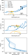 |
Fig. 6 scCHIMERA radiative-convective-chemical equilibrium models where TiO and VO are assumed to have rained out of the atmosphere, along with the planet-to-star flux ratios from CHEOPS (orange), TESS (yellow), and Spitzer (black). The models are all for dayside-only redistribution (f=2) and varying metallicity. High albedo is obtained only at high metallicity through the condensation of MgSiO3. The base of the silicate clouds is shown as a dot in the PT profile. When no dots are shown, the silicate does not form. Kzz was set to 109 cm2/s and fsed was set to 0.1, favoring small more reflective particles. |
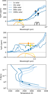 |
Fig. 7 scCHIMERA radiative-convective-chemical equilibrium models. These models include TiO and VO when local chemical equilibrium predicts their presence. The other model parameters and the planet-to-star flux ratios shown are the same as in Figure 6. |
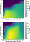 |
Fig. 8 χ2 maps between our models and the CHEOPS data point for chemical equilibrium models (bottom) and models where TiO and VO have rained out of the atmosphere (top). The contour shows the region that agrees with the data within 3 σ. The rainout of TiO and VO allows an easier condensation of the silicate clouds, and thus a high albedo at lower metallicities than for the case in chemical equilibrium. |
5 Discussion and conclusions
This work is aimed at constraining the physical and chemical properties of the extreme Neptunian desert planet LTT9779b, using secondary eclipse observations taken using CHEOPS. First, we used the TESS observations from three sectors (1, 29, and 69) to reanalyze the transit properties and update all physical parameters, including the ephemeris. Since these parameters are directly used for modeling the secondary eclipse observations, as well as the emission and transmission spectroscopic modeling of the atmospheric properties, they are essential updates. Given that LTT9779b is one of the most unique and interesting targets for a plethora of future follow-up studies, these updated parameters will be beneficial not only for the present work, but also for several future studies. Our analysis of the transit light curves included a robust algorithm focused on reducing the impact of various noise components in the parameter estimations. This included techniques such as wavelet denoising and GP regression, which can effectively reduce the time-uncorrelated and time-correlated noise components in the light curves.
In the next step, our ten new secondary eclipse observations from CHEOPS were analyzed, in combination with ten already published observations from CHEOPS, which were previously reported by our team Hoyer et al. (2023). In addition to using the reduced time series data provided by the official CHEOPS data reduction pipeline (DRP), we also reduced the raw data using a completely independent pipeline, PIPE, which used the PSF photometry method. The roll-angle-dependent background contaminations in the CHEOPS light curves were modeled using an N-order glint function implemented within PYCHEOPS, and subtracted from the light curves simultaneously with the secondary eclipse modeling. The two sets of detrended light curves and the estimated secondary eclipse depths, obtained through the two independent data reduction procedures, were found to be in excellent statistical agreement. Thus, it helped us to cross-verify the robustness of our analyses, which is essential for this type of study involving the detection of small and noise-sensitive signatures from observed data. Our analysis with the extended dataset helped us to constrain the secondary eclipse depth of LTT9779b with significantly higher precision than was reported previously in Hoyer et al. (2023), which also resulted in a more robust and precise estimation of its geometric albedo.
Armed with this new and precise eclipse measurement, we were able to re-run our atmospheric models with more realistic physical processes included, all of which confirmed the presence of a high-metallicity atmosphere for the planet. Furthermore, we found difficulties when trying to model the highly reflective optical output and the strong thermal NIR output simultaneously, and we suggest possible ways forward to circumvent these issues. However, regardless of whether more detailed models are applied, the atmosphere has to be significantly enriched in metals when compared to the Sun, and likely the planet hosts a high-altitude silicate cloud layer. These new constraints help further elucidate the formation and evolution history of this planet since a metallic atmosphere with silicate clouds that reflect away 70% of the infalling radiation likely helps to maintain the planet cooler than expected if it were as opaque as the vast majority of hot Jupiters (Hoyer et al. 2023; Radica et al. 2024). Furthermore, as discussed in Vissapragada et al. (2024), a highly metallic atmosphere argues for a smaller atmospheric scale height, which decreases the evaporation rate and increases the cooling rate of any atmospheric outflow. Such cooling processes could help explain why the planet has not lost all of its atmosphere at this time, becoming another bare hot rock super-Earth. As the first planet of its type to be studied in such detail, LTT9779b continues to serve as a benchmark example, with new physical processes being actively teased out from the detailed follow-up observations targeting its atmosphere.
Acknowledgements
We thank the anonymous reviewer for their valuable suggestions, which helped improve the manuscript. SS acknowledges Fondo Comité Mixto-ESO Chile ORP 025/2022 to support this research. The computations presented in this work were performed using the Geryon-3 supercomputing cluster, which was assembled and is maintained using funds provided by the ANID-BASAL Center FB210003, Center for Astrophysics and Associated Technologies, CATA. This paper includes data collected by the TESS mission, which are publicly available from the Mikulski Archive for Space Telescopes (MAST). I acknowledge the use of public TOI Release data from pipelines at the TESS Science Office and at the TESS Science Processing Operations Center. Funding for the TESS mission is provided by NASA’s Science Mission directorate. Support for MAST is provided by the NASA Office of Space Science via grant NNX13AC07G and by other grants and contracts. This paper includes data collected by the CHEOPS mission. CHEOPS is an ESA mission in partnership with Switzerland with important contributions to the payload and the ground segment from Austria, Belgium, France, Germany, Hungary, Italy, Portugal, Spain, Sweden, and the United Kingdom. The CHEOPS Consortium would like to gratefully acknowledge the support received by all the agencies, offices, universities, and industries involved. Their flexibility and willingness to explore new approaches were essential to the success of this mission. CHEOPS data analyzed in this article will be made available in the CHEOPS mission archive (https://cheops.unige.ch/archive_browser/).
Appendix A Figures showing all modeled light curves
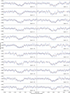 |
Fig. A.3 The normalized transit light curves before (light blue) and after (blue) wavelet denoising, along with the best-fit transit models (brown) (part 1 of 4). |
References
- Ackerman, A. S., & Marley, M. S., 2001, ApJ, 556, 872 [Google Scholar]
- Benz, W., Broeg, C., Fortier, A., et al. 2021, Exp. Astron., 51, 109 [Google Scholar]
- Borucki, W. J., Koch, D., Basri, G., et al. 2010, Science, 327, 977 [Google Scholar]
- Brandeker, A., Heng, K., Lendl, M., et al. 2022, A&A, 659, L4 [NASA ADS] [CrossRef] [EDP Sciences] [Google Scholar]
- Brandeker, A., Patel, J. A., & Morris, B. M., 2024, PIPE: Extracting PSF photometry from CHEOPS data, Astrophysics Source Code Library [record ascl:2404.002] [Google Scholar]
- Caldwell, D. A., Tenenbaum, P., Twicken, J. D., et al. 2020, RNAAS, 4, 201 [NASA ADS] [Google Scholar]
- Collier-Cameron, A., Horne, K., James, D., Penny, A., & Semel, M., 2004, in IAU Symposium, 202, Planetary Systems in the Universe, ed. A. Penny, 75 [Google Scholar]
- Coulombe, L.-P., Benneke, B., Challener, R., et al. 2023, Nature, 620, 292 [NASA ADS] [CrossRef] [Google Scholar]
- Coulombe, L.-P., Radica, M., Benneke, B., et al. 2025, arXiv e-prints, [arXiv:2501.14016] [Google Scholar]
- Crossfield, I. J. M., Dragomir, D., Cowan, N. B., et al. 2020, ApJ, 903, L7 [NASA ADS] [CrossRef] [Google Scholar]
- Daubechies, I., 1988, Commun. Pure Appl. Math., 41, 909 [CrossRef] [Google Scholar]
- Daubechies, I., 1992, Ten Lectures on Wavelets (SIAM) [Google Scholar]
- Donoho, D., & Johnstone, I., 1994, in Ideal Denoising in an Orthonormal Basis Chosen from a Library of Bases [Google Scholar]
- Dragomir, D., Crossfield, I. J. M., Benneke, B., et al. 2020, ApJ, 903, L6 [NASA ADS] [CrossRef] [Google Scholar]
- Edwards, B., Changeat, Q., Tsiaras, A., et al. 2023, AJ, 166, 158 [NASA ADS] [CrossRef] [Google Scholar]
- Esteves, L. J., De Mooij, E. J. W., & Jayawardhana, R., 2015, ApJ, 804, 150 [Google Scholar]
- Fortney, J. J., Lodders, K., Marley, M. S., & Freedman, R. S., 2008, ApJ, 678, 1419 [CrossRef] [Google Scholar]
- Hastings, W., 1970, Biometrika, 57, 97 [NASA ADS] [CrossRef] [Google Scholar]
- Hoyer, S., Guterman, P., Demangeon, O., et al. 2020, A&A, 635, A24 [NASA ADS] [CrossRef] [EDP Sciences] [Google Scholar]
- Hoyer, S., Jenkins, J. S., Parmentier, V., et al. 2023, A&A, 675, A81 [NASA ADS] [CrossRef] [EDP Sciences] [Google Scholar]
- Jenkins, J. M., Twicken, J. D., McCauliff, S., et al. 2016, SPIE Conf. Ser.,. 9913, 99133E [Google Scholar]
- Jenkins, J. S., Díaz, M. R., Kurtovic, N. T., et al. 2020, Nat. Astron., 4, 1148 [Google Scholar]
- Johnson, M. C., Cochran, W. D., Collier Cameron, A., & Bayliss, D., 2015, ApJ, 810, L23 [Google Scholar]
- Krenn, A. F., Lendl, M., Patel, J. A., et al. 2023, A&A, 672, A24 [NASA ADS] [CrossRef] [EDP Sciences] [Google Scholar]
- Lee, G. R., Gommers, R., Waselewski, F., Wohlfahrt, K., & O’Leary, A., 2019, J. Open Source Softw., 4, 1237 [NASA ADS] [CrossRef] [Google Scholar]
- Leigh, C., Collier Cameron, A., Horne, K., Penny, A., & James, D., 2003a, MNRAS, 344, 1271 [Google Scholar]
- Leigh, C., Collier Cameron, A., Udry, S., et al. 2003b, MNRAS, 346, L16 [Google Scholar]
- Line, M. R., Stevenson, K. B., Bean, J., et al. 2016, AJ, 152, 203 [NASA ADS] [CrossRef] [Google Scholar]
- Line, M. R., Brogi, M., Bean, J. L., et al. 2021, Nature, 598, 580 [NASA ADS] [CrossRef] [Google Scholar]
- Luo, G., & Zhang, D., 2012, Wavelet Denoising, Advances in Wavelet Theory and Their Applications in Engineering, Physics and Technology, ed. D. Baleanu (InTech) [Google Scholar]
- Mandel, K., & Agol, E., 2002, ApJ, 580, L171 [Google Scholar]
- Mansfield, M., Line, M. R., Bean, J. L., et al. 2021, Nat. Astron., 5, 1224 [CrossRef] [Google Scholar]
- Maxted, P. F. L., Ehrenreich, D., Wilson, T. G., et al. 2022, MNRAS, 514, 77 [NASA ADS] [CrossRef] [Google Scholar]
- Neath, A. A., & Cavanaugh, J. E., 2012, Wiley Interdiscipl. Rev.: Computat. Statist., 4, 199 [Google Scholar]
- Pagano, I., Scandariato, G., Singh, V., et al. 2024, A&A, 682, A102 [NASA ADS] [CrossRef] [EDP Sciences] [Google Scholar]
- Parmentier, V., Showman, A. P., & Lian, Y., 2013, A&A, 558, A91 [NASA ADS] [CrossRef] [EDP Sciences] [Google Scholar]
- Parmentier, V., Fortney, J. J., Showman, A. P., Morley, C., & Marley, M. S., 2016, ApJ, 828, 22 [Google Scholar]
- Parmentier, V., Line, M. R., Bean, J. L., et al. 2018, A&A, 617, A110 [NASA ADS] [CrossRef] [EDP Sciences] [Google Scholar]
- Pereira, F., Campante, T. L., Cunha, M. S., et al. 2019, MNRAS, 489, 5764 [NASA ADS] [CrossRef] [Google Scholar]
- Quan, P., Lei, Z., Guanzhong, D., & Hongai, Z.., 1999, IEEE Trans. Signal Process., 47, 3401 [Google Scholar]
- Radica, M., Coulombe, L.-P., Taylor, J., et al. 2024, ApJ, 962, L20 [NASA ADS] [CrossRef] [Google Scholar]
- Radica, M., Taylor, J., Wakeford, H. R., et al. 2025, MNRAS, 538, 1853 [Google Scholar]
- Ramírez Reyes, R., Jenkins, J. S., Sedaghati, E., et al. 2025, A&A, 695, A26 [NASA ADS] [CrossRef] [EDP Sciences] [Google Scholar]
- Rasmussen, C. E., & Williams, C. K. I., 2006, Gaussian Processes for Machine Learning (The MIT Press) [Google Scholar]
- Ricker, G. R., Winn, J. N., Vanderspek, R., et al. 2015, J. Astron. Telesc. Instrum. Syst., 1,014003 [Google Scholar]
- Roth, A., Parmentier, V., & Hammond, M., 2024, MNRAS, 531, 1056 [CrossRef] [Google Scholar]
- Rowe, A. C. H., & Abbott, P. C., 1995, Comput. Phys., 9, 635 [Google Scholar]
- Rowe, J. F., Matthews, J. M., Seager, S., et al. 2008, ApJ, 689, 1345 [Google Scholar]
- Saha, S., 2022, PhD thesis, Indian Institute of Astrophysics [Google Scholar]
- Saha, S., 2023, ApJS, 268, 2 [NASA ADS] [CrossRef] [Google Scholar]
- Saha, S., 2024, ApJS, 274, 13 [Google Scholar]
- Saha, S., 2025, MNRAS, 539, 928 [Google Scholar]
- Saha, S., & Sengupta, S., 2021, AJ, 162, 221 [NASA ADS] [CrossRef] [Google Scholar]
- Saha, S., Chakrabarty, A., & Sengupta, S., 2021, AJ, 162, 18 [CrossRef] [Google Scholar]
- Schwartz, J. C., & Cowan, N. B., 2017, PASP, 129, 014001 [Google Scholar]
- Serrano, L. M., Gandolfi, D., Hoyer, S., et al. 2022, A&A, 667, A1 [Google Scholar]
- Sheets, H. A., & Deming, D., 2017, AJ, 154, 160 [CrossRef] [Google Scholar]
- Showman, A. P., & Guillot, T., 2002, A&A, 385, 166 [NASA ADS] [CrossRef] [EDP Sciences] [Google Scholar]
- Singh, V., Scandariato, G., Smith, A. M. S., et al. 2024, A&A, 683, A1 [NASA ADS] [CrossRef] [EDP Sciences] [Google Scholar]
- Sudarsky, D., Burrows, A., & Pinto, P., 2000, ApJ, 538, 885 [Google Scholar]
- Vissapragada, S., McCreery, P., Dos Santos, L. A., et al. 2024, ApJ, 962, L19 [NASA ADS] [CrossRef] [Google Scholar]
- Wiser, L. S., Line, M. R., Welbanks, L., et al. 2024, ApJ, 971, 33 [Google Scholar]
- Woitke, P., & Helling, C., 2003, A&A, 399, 297 [NASA ADS] [CrossRef] [EDP Sciences] [Google Scholar]
All Tables
Estimated physical properties for LTT9779b from the transit modeling of TESS light curves.
Estimated secondary eclipse depths from the light curves reduced by DRP and PIPE.
All Figures
|
Fig. 1 Observed and best-fit model light curves corresponding to the first transit observed from each TESS sector. For each transit, the top panel shows the unprocessed light curve (light blue), the light curve after wavelet denoising (blue), and the best-fit transit model (brown); the middle panel shows the residual flux before GP regression (blue), and the mean (green) and 1 σ interval (light blue) of the best-fit GP regression model; and the bottom panel shows the final mean residual flux (blue). The mean residual flux corresponds to the residual flux considering the mean of the best-fit GP regression model. |
| In the text | |
|
Fig. 2 Trends in the background flux variations with respect to the roll-angle for the CHEOPS observation corresponding to epoch 1889, from the light curves reduced by the DRP (top) and PIPE (bottom). The light blue points show individual observations (without uncertainties), and the blue points show data binned over 15° intervals. It is worth noting that the trend of variation is different between the light curves reduced using the DRP and PIPE, since PIPE has a different sensitivity to background stars that contaminate the photometric apertures in the DRP outputs. |
| In the text | |
|
Fig. 3 Detrended individual (light blue, without uncertainties) and binned (blue, binned over 7.2 min intervals) secondary eclipse light curves corresponding to epochs 971 and 1889, reduced by using the DRP (top) and PIPE (bottom). The best-fit transit models are shown as brown lines (the green portions show the disruptions in the light curves), and the residuals from the best-fit models in the bottom panels. The light curves reduced by the DRP and PIPE are in statistical agreement with each other. |
| In the text | |
|
Fig. 4 Secondary eclipse depths estimated for each individual epoch from the light curves reduced by the DRP (blue) and PIPE (orange, with a slight offset along the x-axis for visibility), along with the calculated mean secondary eclipse depths (blue and orange dotted lines for the light curves reduced by DRP and PIPE respectively; the shaded regions show the uncertainties). We note that the eclipse depths estimated from the two sets of light curve data reduced by independent pipelines (i.e., DRP and PIPE) are in close statistical agreement with each other. |
| In the text | |
|
Fig. 5 Geometric albedo vs. radius plot for LTT9779b estimated from this work (DRP, red), from Hoyer et al. 2023 (blue), and from Coulombe et al. 2025 (western dayside in green and eastern dayside in violet) also showing the known well-constrained geometric albedos of other hot and ultra-hot Jupiters from the literature (orange). |
| In the text | |
|
Fig. 6 scCHIMERA radiative-convective-chemical equilibrium models where TiO and VO are assumed to have rained out of the atmosphere, along with the planet-to-star flux ratios from CHEOPS (orange), TESS (yellow), and Spitzer (black). The models are all for dayside-only redistribution (f=2) and varying metallicity. High albedo is obtained only at high metallicity through the condensation of MgSiO3. The base of the silicate clouds is shown as a dot in the PT profile. When no dots are shown, the silicate does not form. Kzz was set to 109 cm2/s and fsed was set to 0.1, favoring small more reflective particles. |
| In the text | |
|
Fig. 7 scCHIMERA radiative-convective-chemical equilibrium models. These models include TiO and VO when local chemical equilibrium predicts their presence. The other model parameters and the planet-to-star flux ratios shown are the same as in Figure 6. |
| In the text | |
|
Fig. 8 χ2 maps between our models and the CHEOPS data point for chemical equilibrium models (bottom) and models where TiO and VO have rained out of the atmosphere (top). The contour shows the region that agrees with the data within 3 σ. The rainout of TiO and VO allows an easier condensation of the silicate clouds, and thus a high albedo at lower metallicities than for the case in chemical equilibrium. |
| In the text | |
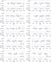 |
Fig. A.1 Same as Figure 3, but for all the light curves reduced by DRP (part 1 of 2). |
| In the text | |
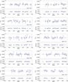 |
Fig. A.2 Same as Figure 3, but for all the light curves reduced by PIPE (part 1 of 2). |
| In the text | |
|
Fig. A.3 The normalized transit light curves before (light blue) and after (blue) wavelet denoising, along with the best-fit transit models (brown) (part 1 of 4). |
| In the text | |
Current usage metrics show cumulative count of Article Views (full-text article views including HTML views, PDF and ePub downloads, according to the available data) and Abstracts Views on Vision4Press platform.
Data correspond to usage on the plateform after 2015. The current usage metrics is available 48-96 hours after online publication and is updated daily on week days.
Initial download of the metrics may take a while.