| Issue |
A&A
Volume 700, August 2025
|
|
|---|---|---|
| Article Number | A119 | |
| Number of page(s) | 19 | |
| Section | Interstellar and circumstellar matter | |
| DOI | https://doi.org/10.1051/0004-6361/202554355 | |
| Published online | 15 August 2025 | |
Narrow absorption lines from intervening material in supernovae
II. Galaxy properties
1
Instituto de Astrofisica e Ciências do Espaço, Faculdade de Ciências, Universidade de Lisboa,
Ed. C8, Campo Grande,
1749-016
Lisbon,
Portugal
2
CENTRA, Instituto Superior Técnico, Universidade de Lisboa,
Av. Rovisco Pais 1,
1049-001
Lisboa,
Portugal
3
European Southern Observatory,
Alonso de Córdova 3107,
Casilla 19,
Santiago,
Chile
4
Institut d’Estudis Espacials de Catalunya (IEEC),
Edifici RDIT, Campus UPC,
08860
Castelldefels (Barcelona),
Spain
5
Institute of Space Sciences (ICE, CSIC),
Campus UAB, Carrer de Can Magrans, s/n,
08193
Barcelona,
Spain
6
School of Physics, Trinity College Dublin, The University of Dublin,
Dublin 2,
Ireland
7
Millennium Institute of Astrophysics MAS,
Nuncio Monsenor Sotero Sanz 100, Off. 104,
Providencia,
Santiago,
Chile
8
School of Physics and Astronomy, University of Southampton,
Southampton,
SO17 1BJ,
UK
9
Department of Applied Physics, School of Engineering, University of Cádiz,
Campus of Puerto Real,
11519
Cádiz,
Spain
10
Instituto de Astrofísica de Andalucía - CSIC,
Apdo 3004,
18080
Granada,
Spain
11
Tuorla Observatory, Department of Physics and Astronomy, University of Turku,
20014
Turku,
Finland
12
European University Cyprus,
Diogenes Street, Engomi,
1516
Nicosia,
Cyprus
★ Corresponding authors: This email address is being protected from spambots. You need JavaScript enabled to view it.
; This email address is being protected from spambots. You need JavaScript enabled to view it.
Received:
3
March
2025
Accepted:
17
June
2025
Abstract
The interstellar medium (ISM) has a number of tracers such as the NaI Dλλ 5890, 5896 absorption lines that are evident in the spectra of galaxies but also in those of individual astrophysical sources such as stars, novae, or quasars. Here, we investigate narrow absorption features in the spectra of nearby supernovae (SNe) and compare them to local (<0.5 kpc) and global host galaxy properties. With a large and heterogeneous sample of spectra, we are able to recover the known relations of ISM with galaxy properties: larger columns of ISM gas are found in environments that are more massive, more actively star-forming, younger, and viewed from a more inclined angle. Most trends are stronger for local properties than global properties, and we find that the ISM column density decreases exponentially with the offset from the host galaxy centre, as expected for a gas distribution following an exponential radial profile. We also confirm trends for the velocity of galactic outflows increasing with radius. The current study demonstrates the capability of individual light sources to serve as ubiquitous tracers of ISM properties across various environments and galaxies.
Key words: supernovae: general / dust, extinction / ISM: lines and bands
© The Authors 2025
 Open Access article, published by EDP Sciences, under the terms of the Creative Commons Attribution License (https://creativecommons.org/licenses/by/4.0), which permits unrestricted use, distribution, and reproduction in any medium, provided the original work is properly cited.
This article is published in open access under the Subscribe to Open model. This email address is being protected from spambots. You need JavaScript enabled to view it. to support open access publication.
1 Introduction
The interstellar medium (ISM) of galaxies plays a crucial role in providing the constituents for forming new stars, the reservoir for dying stars, and other galactic processes such as feedback and fuelling of active galactic nuclei. The ISM thus regulates the galactic chemical enrichment and the star formation history of galaxies. The cold ISM responsible for star formation represents approximately 10-20% of the total baryon content (gas and stars) of a late-type galaxy similar to the Milky Way (Draine 2011). Most of this cold ISM (~75%) consists of atomic gas, essentially hydrogen, with the rest in molecular form. Dust, responsible for the absorption and scattering of light bluewards of the optical regime and re-emission redwards of the infrared, constitutes 1% of the gas mass, but is an excellent tracer of the atomic and molecular ISM. For early-type galaxies, the ISM content is rather low at ~3% of the total baryonic mass (Saintonge & Catinella 2022).
Heavier elements are also mixed together with the atomic hydrogen and absorb the light of background sources at characteristic wavelengths. Therefore, it is possible to study the ISM gas content and its kinematics with absorption-line spectroscopy of atomic ions. The sodium doublet lines (NaI D λλ5890, 5896) are among the strongest absorption lines in galaxy spectra. Other atomic lines include ionised calcium (CaIIH & K λλ 3970, 3935) and neutral potassium (KIλλ 7665, 7669). The strength of these lines, particularly sodium, strongly correlates with gas phase and dust attenuation, together with galaxy inclination, stellar mass, and star formation rate (Chen et al. 2010). The kinematics of the lines, on the other hand, can reveal important information on galactic outflows and their relation to galactic properties (Rupke et al. 2005b; Chen et al. 2010; Park et al. 2015; Cazzoli et al. 2022).
Studies of ISM absorption lines have traditionally relied on galaxy spectra with the galaxy continuum as the background source of light. This leads to the complication of having a contribution of stellar atmospheres in the absorption lines. Such contamination can even reach ~80% in cool stars (Chen et al. 2010). There are mechanisms to correct for the stellar component, for example through the correlation of stellar sodium with magnesium lines (MgI triplet λλ 5167, 5173, 5184) only present in stars (Martin 2005; Rupke et al. 2005a) or through stellar population fits to the continuum to obtain the stellar part (Chen et al. 2010). However, both methods have drawbacks and large uncertainties.
Absorption lines of the atomic ISM are also present in the spectra of other background sources such as resolved single stars in molecular clouds (e.g. Pascucci et al. 2015), novae (e.g. Jack & Schröder 2019), or quasars (e.g. Boissé et al. 2015; Kacprzak et al. 2015). Supernovae (SNe), bright stellar explosions, are particularly suitable lighthouses, as they occur in various environments and are so bright that they may outshine their neighbourhood or even their entire host galaxy. Their spectra are known to present absorption lines from the ISM, notably sodium, but also potassium, calcium, and diffuse interstellar bands (DIBs; e.g. Sollerman et al. 2005; Gutiérrez et al. 2016), which have been used as tracers of gas and as proxies of dust extinction (e.g. Welty et al. 2014; Ritchey et al. 2015), even in extreme environments (e.g. tidal tails; Ferretti et al. 2017). Therefore, absorption lines in SN spectra can serve as probes of the local ISM content at individual sight lines with the advantage that there is a negligible contribution from stellar populations in their spectra (although see Kangas et al. 2016). Furthermore, the ISM lines are narrow and easily distinguishable from the intrinsic SN ejecta component, which has a characteristic broad P Cygni profile. Nevertheless, care should be taken when using low-resolution spectroscopy as this broad profile may affect the measurement of the ISM lines (González-Gaitân et al. 2024, hereafter Paper I).
A disadvantage of using SNe to study the ISM is the influence on the lines of very nearby circumstellar material (CSM) ejected by the progenitor system before the explosion, which is not representative of the ISM. CSM signatures are clearly seen in the strength and evolution of Balmer emission lines in interacting SNe, particularly Ha (e.g. Chugai & Danziger 1994; Chevalier & Fransson 1994; Fransson et al. 2002; Dessart et al. 2023), and also in the absorption line strengths of gas atoms such as sodium in intermediate-luminosity red transients (Byrne et al. 2023). However, for most SNe these lines are essentially constant throughout their evolution (Paper I). A handful of well-studied exceptions show variation (Patat et al. 2007; Blondin et al. 2009; Simon et al. 2009; Graham et al. 2015; Ferretti et al. 2016), and there is a fraction of SNe with excess sodium absorption strength that is also blueshifted (Sternberg et al. 2011; Phillips et al. 2013; Maguire et al. 2013; Hachinger et al. 2017). This may indicate outflows from the progenitor system or nearby ISM clouds accelerated by the SN radiation (Hoang et al. 2019; Bulla et al. 2018).
In Paper I, we developed a robust automated technique to measure the narrow lines of ISM tracers from SN spectra of various resolutions, showing the limitations of low-resolution spectra and how to circumvent these constraints. We also applied the methodology to a large sample of SNe to investigate the evolution of the lines throughout the SN lifetime, and found no statistically significant change in those lines. For this paper, we used the same large heterogeneous sample presented in Paper I of nearby SNe occurring at multiple locations and in different galaxy types to study the spectroscopic absorption lines of ISM tracers as a function of various galaxy properties. To our knowledge, this is the first time that individual point sources have been used as possible generic large-scale tracers of resolved ISM properties within galaxies and across multiple galaxies of different types and characteristics. We aim to gauge if SNe can truly be used as universal tracers of ISM properties. The paper is organised as follows. Section 2 describes our methodology. The analysis and results are presented in Section 3 and discussed in Section 4, while our conclusions are presented in Section 5. In a companion paper (Paper III), we put constraints on the nature of the progenitor systems of the different SN types by using the known galaxy relations on the ISM gas composition, distribution, and kinematics.
Number of SNe used in this study.
2 Methodology
This section outlines the methodology and analysis and introduces the data used for this study. A detailed description of the data and SN measurements can be found in Paper I.
2.1 SN EW measurements
The public SN sample used in the present study consists of a large heterogeneous nearby spectroscopic dataset obtained by multiple surveys. It initially consisted of thousands of spectra of nearly 1300 SNe of different types. Table 1 summarises the number of SNe used. For a full list of the sample, see Table A.1 of Paper I.
To characterise the narrow interstellar absorption lines observed in SNe spectra, we measured their equivalent widths (EWs) and velocities (VELs). The algorithm to measure the EW first finds the continuum by smoothing the flux with a cosine kernel; then, the EW is obtained by calculating the area under/over the continuum within a given window. The velocity is determined from the weighted average wavelength shift from the rest frame according to the area under/over the continuum. In the case of multiple spectra for a given SN, a stacked flux-to-continuum spectrum is obtained from which the EW and VEL are measured, and a bootstrap of 100 realisations gives the statistical uncertainty. We made sure that the signal-to-noise (S/N) of the individual spectra is large enough (S/N > 15) and that the continuum slope is not too steep to avoid the underlying P Cygni profile of the SN ejecta affecting the narrow line. We refer to Paper I for more details. In Appendix A, we compare the different lines to each other, whereas in Appendix B, the EW and VEL of the lines are compared.
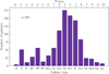 |
Fig. 1 Galaxy type distribution of our SN sample. n = 985 is the number of SN host galaxies. |
2.2 Galaxy properties
The host galaxies of the SN sample are nearby (z≲0.2) and have abundant public information. We obtained the spectroscopic redshift, the right ascension and declination, the morphological type and the semi-major/minor axes, a and b, from the NASA/IPAC Extragalactic Database (NED) database1. The galaxy type was complemented with the Asiago catalogue2 information (Barbon et al. 2010) and transformed to a T-type (de Vaucouleurs 1959) number between −6 and 10. Figure 1 shows the galaxy T-type distribution for our sample. Our SNe cover a large diversity of environments, going from passive to starforming galaxies. The peak of the distribution is around the Sb type, corresponding to the T-type of 3.
From the SN and host galaxy (GAL) co-ordinates, we obtained the angular offset
 (1)
(1)
with
![Mathematical equation: \begin{eqnarray*} \Delta\mathrm{Ra} &=& (\mathrm{Ra}_\mathrm{SN}-\mathrm{Ra}_\mathrm{GAL})\cos{\left[0.5(\mathrm{Dec}_\mathrm{SN}+\mathrm{Dec}_\mathrm{GAL})\right]} \\ \Delta\mathrm{Dec} &=& \mathrm{Dec}_\mathrm{SN}-\mathrm{Dec}_\mathrm{GAL}. \end{eqnarray*}](/articles/aa/full_html/2025/08/aa54355-25/aa54355-25-eq2.png)
We define the unit-less normalised offset, Δα, by dividing the angular offset by the semi-major axis (a) of the galaxy (see Fig. 2). This normalisation considers the galaxy’s size, but also reduces the effect of the distance of the galaxy:
 (2)
(2)
A more accurate normalisation of the angular separation takes into account the host ellipse axis size in the direction of the SN, the so-called directional light radius, dDLR (Sullivan et al. 2006; Gupta et al. 2016; Gagliano et al. 2021) given by
 (3)
(3)
where a and b are the semi-major and semi-minor axes, while β, the angle subtended between the galaxy semi-major axis and the line connecting the SN to the galactic centre, is given by with φ being the angular tilt of the ellipse with respect to the celestial north. The final normalised separation is
 (4)
(4)
The inclination of spiral galaxies is estimated following Hubble (1926), and assuming that the disk is circular when viewed face-on and with a finite thickness:
 (5)
(5)
Here q = b/a is the ratio of the semi-minor to semi-major axes and q0 is the intrinsic axis ratio when viewed edge-on (Fouque et al. 1990). We assume a universal q0 = 0.2 (Holmberg 1946; Ho et al. 2011; Noordermeer & van der Hulst 2007) although it has been shown to vary with galaxy type, mass and luminosity (Heidmann et al. 1972; Bottinelli et al. 1983; Yuan & Zhu 2004; Rodríguez & Padilla 2013).
As explained in the next sections, we also considered stellar parameters derived from stellar populations that fit local and global photometry. Table 2 lists all the galaxy properties considered in this study.
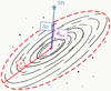 |
Fig. 2 Sketch of a spiral galaxy3 with the SN (blue star) indicating as a blue line the angular offset with the host centre Δα, in red the semimajor axis a of the ellipse, and in purple the directional light radius dDLR. |
2.2.1 Galaxy photometry
The SNe in our sample occurred in nearby galaxies (0.004 < z < 0.2), for which there is extensive literature photometry. We used public optical images either from the Dark Energy Survey (DES; Abbott et al. 2018; Abbott et al. 2021; Morganson et al. 2018; Flaugher et al. 2015), Pan-STARRS1 (PS1; Waters et al. 2020; Magnier et al. 2020; Flewelling et al. 2020) or from the Sloan Digital Sky Survey (SDSS; Abdurro’uf et al. 2022), ultraviolet (UV) photometry from the NASA Galaxy Evolution Explorer (GALEX; Morrissey et al. 2008; Bianchi et al. 2014), near-infrared (NIR) images either from the Two Micron All Sky Survey (2MASS; Skrutskie et al. 2006) or from the Visible and Infrared Survey Telescope for Astronomy (VISTA; McMahon et al. 2013; Irwin et al. 2004; Lewis et al. 2010; Cross et al. 2012), and infrared imaging from the unblurred co-adds of the Wide-field Infrared Survey Explorer (unWISE; Lang 2014; Meisner et al. 2017a,b). We required one optical dataset, giving preference to DES over PS1 over SDSS, if available, and one NIR dataset, prioritising VISTA over 2MASS because of their higher resolution. The list of surveys and filters used is shown in Table 3.
To download the images and perform photometry, we used the software HOSTPHOT4 (Müller-Bravo & Galbany 2022) tailored to SN host galaxies. The images were first masked for foreground stars cross-matched to the Gaia catalogue (Gaia Collaboration 2016, 2023). We then obtained global photometry in each filter image using Kron apertures (Kron 1980) defined on the stack of the optical filters (see Figure 3).
Local photometry was performed with circular apertures of radii of 0.5 kpc centred at the SN position (see Figure 4). The physical apertures were obtained with the redshift, assuming a standard cosmology (H0 = 70 km/s/Mpc and Ωm = 0.3). Since most of the optical images we used come from the SDSS, which has a lower resolution than DES, we set an upper redshift limit of 0.02, corresponding to a radial aperture of 0.5 kpc with the typical SDSS seeing of 1.2″. Higher redshifts had an aperture below the seeing limit and were not considered. The number of SNe with global and local photometry was reduced to 613 and 357, respectively (see Table 1).
Galaxy properties studied.
Surveys and filters for SN host photometry.
2.2.2 Spectral energy distribution fitting
We used PROSPECTOR5 (Johnson et al. 2021; Leja et al. 2017) to fit stellar populations to the non-zero fluxes of the available filters of our local and global host galaxy photometry obtained with hostphot. The composite stellar populations were built with FSPS (Conroy & Gunn 2010; Conroy et al. 2009) using the MIST isochrones (Dotter 2016; Choi et al. 2016; Paxton et al. 2015, 2013, 2011) and the MILES spectral library (Falcón-Barroso et al. 2011), with a Kroupa initial mass function (Kroupa 2001) and a delayed-τ star formation history given by a star formation rate (SFR) as a function of lookback time, t,
 (6)
(6)
where tage and τ are the age and the characteristic e-folding time in Gyr of the star-forming episode, both free parameters of the fit along with the stellar metallicity (Z*/Z⊙), and the stellar mass of existing stars and stellar remnants (M*/M⊙). Although this treatment of the star formation history is simplistic and may fail to reproduce the extremes of galaxy populations (Simha et al. 2014), the relative differences among populations - our main focus - are overall maintained. We used a diffuse dust attenuation given by Noll et al. (2009) with two free parameters, the total dust attenuation τv or ‘dust2’, related to the optical depth and AV, and the dust attenuation index n which controls the wavelength dependence,
![Mathematical equation: \tau(\lambda) = \frac{\tau_V}{R_{V,0}}[k(\lambda)+D(\lambda)]\left(\frac{\lambda}{\lambda_V}\right)^n,](/articles/aa/full_html/2025/08/aa54355-25/aa54355-25-eq22.png) (7)
(7)
where k(λ) is the attenuation curve of Calzetti et al. (2000), with Rv,0 = 4.05, and D(λ) accounts for the UV-bump Drude profile.
We thus have six free parameters: tage, τ, Z*, M„ τV and n. Additionally, the recent star formation rate (SFR0), averaged over the last 100 Myr, can be directly obtained from Eq. (6). Thus, the recent specific star formation rate (sSFR0) was defined as
 (8)
(8)
The parameter space was sampled with a Markov chain Monte Carlo (Foreman-Mackey et al. 2013) of 2512 iterations and 128 walkers. The starting point is given by a distribution around the best-fit parameters of ten initial optimisations. A burn-in of 852 steps ensures the parameters have converged in most cases, but we do a visual check and extend the burn-in and iterations when necessary. If the fits are still visually unsatisfactory, these SNe are removed from the analysis (6% of the sample). The best-fit spectral energy distribution (SED) for two representative galaxies and their corresponding corner plots are presented in Figures 5 and 6, respectively. As seen in Figure 5, the reddest WISE filters, particularly W4 (22 μm), tend to show higher fluxes than the models, perhaps due to a contribution from dust emission that is not modelled here. Also, as seen in Figure 6, given its large uncertainties, the e-folding time τ was not always well constrained.
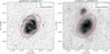 |
Fig. 3 Representative HOSTPHOT images of SN 2001ed with the filters: FUV (GALEX) and W2 (unWISE). Masked sources are shown in grey, and the global Kron apertures are shown as red ellipses. The galaxy centre is shown as a purple cross, whereas the SN position is a cyan star. |
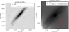 |
Fig. 4 Representative HOSTPHOT images of SN 2001el with the filters: zDECam (DES) and JVISTA (VISTA). Masked sources are shown in grey, and the local circular apertures for r = 0.5 kpc are shown as red lines. The cyan star denotes the SN position. We note that the images have different orientations and resolutions. |
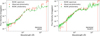 |
Fig. 5 PROSPECTOR SED fits to the observed global photometry of the host galaxy of SN 2010H (left) and local photometry of the host galaxy of SN 2002bf (right). The observed photometry is shown with orange circles with corresponding filter names. The median MCMC fit is shown in dark green with synthetic photometry as green squares, and 100 MCMC realisations are shown in light green. |
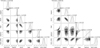 |
Fig. 6 Corner plots resulting from PROSPECTOR SED fits to the observed global/local photometry of the host galaxy of SN 2010H/SN 2002bf (left/right). The six free parameters (logM*, logZ*, τv or dust2, tage, log τ, and dust index n) are shown in each panel. |
2.2.3 Sample comparison
The final stellar mass M*, SFR and sSFR parameters of our sample obtained from global photometry are shown in Figure 7. For comparison, we show the distributions of the SDSS galaxies from the MPA/JHU catalogue6. The SDSS stellar masses were obtained from photometric fits (following Kauffmann et al. 2003; Salim et al. 2007)7, and they covered a similar range to our sample (left panel). The SFR (middle panel) and sSFR (right panel) values, on the other hand, were obtained with spectral line diagnostics (Brinchmann et al. 2004); therefore, a direct comparison with our stellar fits is more difficult. With that in mind, we see clear differences towards more strongly starforming galaxies in our low-z sample. This could be due in part to known overestimates in the SFR integrated over short time periods of 100 Myr (Boquien et al. 2014). On the other hand, our nearby targeted sample is likely comprised of larger, brighter star-forming galaxies. For the purpose of our study, absolute shifts are irrelevant since we care only about relative differences within the sample.
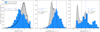 |
Fig. 7 Stellar mass (left), SFR (middle), and sSFR (right) distributions of our sample (blue) compared with the SDSS measurements (grey) from the MPA/JHU catalogue. The vertical dashed lines mark the median values for each distribution. |
3 Analysis and results
In this section, we compare the EW and VEL distributions of the narrow interstellar NaI D line measured for the SN sample presented in Section 2.1 and their corresponding galaxy properties obtained in Section 2.2. To this end, we generate cumulative distributions to test whether two samples, divided based on a given galaxy property, originate from the same parent EW/VEL distribution using the Kolmogorov-Smirnov (K-S) statistic (Kolmogorov 1933; Smirnov 1939)8. If the K-S test has a p-value ρKS < 0.05 (ρKS < 0.01), then the null hypothesis that the two populations are drawn from the same distribution can be marginally (strongly) rejected. To test the robustness of these tests against outliers in the sample, we also do a bootstrap, generating 1000 random sub-samples from which we calculate the probability that the K-S test p-value is less than 0.05. Since our sample is incomplete, we also ensure that the redshift distributions of the two samples are consistent in each bootstrap iteration. This is done first by obtaining the optimal redshift bins (via Bayesian Blocks, see Scargle et al. 2013) and drawing from each of these bins several SNe in one sample that are within the Poisson error of the other sample. We call this a “z-matched” bootstrap K-S test. Moreover, since the division of the two samples can be rather arbitrary, instead of using only the median of the galaxy property to obtain the two samples to be tested, we do a sweep of 10 different dividing values around the median (from 40 to 60% percentile of the distribution). For each division point, we do the z-matched bootstrap so that at the end, we have 10 × 1000 = 10000 realisations of the K-S test. The final value we quote is the median of all these iterations and the corresponding probability of the p-value being less than 0.05. Although using the minimum K-S test instead of the median (see Förster et al. 2013) would provide the best division at which the samples are most different from each other, our approach is more robust to statistical fluctuations. In Appendix C, we also show the K-S tests based on the lower and upper quartiles of each distribution, as well as considering the look-elsewhere effect. Finally, to be certain that any differences between samples are not coming from measurement biases, we always check the K-S test obtained by measuring the same lines but at the wavelengths corresponding to the redshift of the Milky Way (MW), for which we expect the populations to be fully consistent.
We start by dividing each galaxy property into two samples based on its median and then comparing the two samples’ EW (or VEL) distributions. We also analyse if the EW (or VEL) correlates with each property via the non-parametric Spearman’s rank coefficient, rs (Spearman 1904). The K-S statistics and correlations for NaI D EW distributions divided according to galaxy properties are presented in Table 4 and Figure 9. Many of the properties present strong K-S test statistics, as highlighted in bold, according to their z-matched bootstrap probability of being drawn from different parent populations, i.e. probability higher than 50% of a K-S p-value less than 0.05: P(pMC < 0.05) > 50%. The strongest K-S rejections are found for the offset of the SN from the host galaxy centre, especially when normalised by the semi-major axis of the galaxy. In this case, the median bootstrap K-S p-value is ~10−20 or a 100% MC probability that the two NaI D EW distributions of low and high normalised offset are not drawn from the same distribution. Since the relation is so strong, we further divide the sample into four equal offset bins as shown in the left Figure 8: all four samples are statistically different according to the K-S tests. This can be further seen in the right scatter plot, where clearly the EW values inside 25% of the galaxy’s major axis cover a wider range, extending to values as high as 4-5 A. At high separations from the centre, the lines are, on average, weaker. We caution that the offset range seen in Figure 8 may seem shifted to low values (the majority of values are below the semi-major axis, i.e.  ) compared with separations in the literature. This is due to the large semi-major axes from NED as compared to those from Kron apertures, for example, used to normalise the angular offsets (see Appendix D). Although the K-S tests still show significant differences between the samples for the angular offset (~ 10−7) and the DLR offset (~10−14), they are weaker than the normalised offset. The normalised offset is normalised by the semi-major axis and washes out any distance uncertainties, as well as different galactic sizes. The DLR also normalises by the ellipse axis into the SN direction and has shown to be the most robust parameter for SN host galaxy association (Gupta et al. 2016); however, all our tests with narrow lines are stronger for the normalised offset. This is likely because the DLR partly washes out the galactic inclination, as explained in the following paragraph. For this reason, we focus only on the normalised offset in the remainder of the paper.
In addition to the offset location from the galaxy, we find strong evidence for a difference between the EW of the NaI D doublet among morphological galaxy types, with a median K-S p-value of 10−6 (or 100% probability of being different), passive galaxies host SNe with less sodium absorption. In comparison, younger spirals tend to have stronger absorption. The inclination of the galaxy also plays a substantial role in differentiating the column density of sodium gas: as expected in highly inclined galaxies (viewed edge-on), the column density is significantly higher than in less inclined hosts (viewed face-on) as given by a K-S p-value of ~10−4 (PMC = 98%). As the DLR considers both semi-major and semi-minor axes to get the vector distance to the SN position, it includes the inclination of the host galaxy partly. By normalising through the DLR, we subtract part of this influence, and that is why the normalised offset is indeed a better tracer of EW. If we do a K-S test for only face-on galaxies with inclinations larger than 70°, we find that the DLR is indeed stronger (D = 0.37, p-value= 4.1 × 10⁻⁴ and PMC = 95%) than the normalised offset (D = 0.34, p-value = 1.8 × 10⁻³ and PMC = 89%), showing that the inclination plays an important role in the EW of SNe.
Regarding the stellar and dust parameters obtained from the local (r = 0.5 kpc) SED fits, we find strong differences (PMC > 80%) in EW distribution for the recent (<100 Myr) star formation rate SFR0L, the stellar mass M*L, the dust attenuation  and dust slope n, the stellar age
  and the specific star formation rate sSFR0L. Higher EWs of NaID are found in star-forming, more massive, younger and dustier (more attenuated) environments. An example for the local SFR is shown in Figure 10, and local stellar mass is shown in Figure 11.
For the global stellar and dust properties, none of the parameters show strong significance. This clearly suggests that the SN narrow line characteristics are indicators of the local galactic environment rather than the global properties of the hosts. Interestingly, of the fitted global properties, the stellar mass seems to be the best indicator of the ISM (PMC = 40%), even more than the dust attenuation (PMC = 21%).
In Table 5, we also show the results for the K-S tests and correlations of the most significant NaI D VEL distributions. We note that the velocities of very weak lines (i.e. EW< |0.3|Å) are very hard to measure and thus not considered in these statistics (see Appendix B). We see that the normalised offset again has the lowest p-value of the K-S test, which can also be seen in Figure 12: high- and low-offset SNe are generally more blue- and redshifted, respectively, with respect to the SN systemic velocity. However, there is a large dispersion, and the correlation between both parameters is weak. In fact, the blueshift is driven mainly by fewer SNe at high offsets. The VEL distributions, divided according to other galaxy properties as well as to the EW, are not significantly different from each other.
Lastly, we confirm some of the trends found with NaI D EW with absorption lines from other species, in particular for Ca ii H&K, the DIB-5780 and Ki divided according to the normalised offset, local SFR and age, and a few other properties shown in Table 6. Interestingly, we find that the distributions of the EW of DIB-5780, divided according to global stellar mass and age, are significantly different. We note that the more significant relations are seen for the lines that are generally stronger (see Table A.1). However, they are generally weaker than NaI D and, in low-resolution spectra, harder to measure.
K-S statistics and correlations for NaI D EW divided according to galaxy properties.
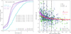 |
Fig. 8 Left : cumulative distributions of NaID EW divided into four bins according to normalised offset. K-S tests indicate that all bins are not drawn from the same distribution. Right: NaI D EW vs normalised offset. SNe located in spirals and ellipticals are highlighted as blue stars and green crosses, respectively. At the top of the figure, n = 667 is the number of events, rS = −0.44 is the Spearman correlation coefficient, and P = 6.3 × 10⁻³³ is the probability of detecting a correlation by chance. The vertical dash-dotted lines represent the 25th, 50th and 75th percentiles of the sample from which the cumulative distributions are obtained. The red dashed line is the rolling median, the purple solid line is the exponential fit to the medians, with the shaded purple area indicating the 1σ uncertainty, and the orange line an exponential function from a symbolic regression (see Sect. 4.2). |
 |
Fig. 9 K-S test p-values (log) of NaID EW divided according to galaxy properties: normalised offset, T-type, inclination, and local stellar and dust properties. |
4 Discussion
We now move to the discussion of the results found in the previous section. We analyse the results of all SNe together as a function of galaxy properties in Section 4.1, trying to find the most relevant relations in Section 4.2. In Section 4.3, we comment on the influence of non-ISM, SN-related physics in the obtained EW and VEL distributions.
Significant K-S statistics and correlations for NaIDVEL divided according to galaxy properties.
4.1 Comparison to previous galaxy studies
This work confirms the findings of multiple ISM characteristics and galaxy properties. Firstly, we find that the column density of ISM lines decreases sharply with galactic radius. Despite the heterogeneous distribution of the ISM structured in gas clouds, H ii regions, voids and filaments, the ISM in spiral galaxies is, on average, distributed in a disk with an exponential profile decreasing with a radius similar to the distribution of stars (e.g. Bianchi 2007; Muñoz-Mateos et al. 2011; Casasola et al. 2017). We also see a qualitative decrease of NaI D EW with radius, as seen in Figure 8, despite the numerous different galaxy types and viewing angles that are showcased. Although the dispersion is too large to allow for a quantitative fit to all SNe, we can perform an exponential fit to the median values, finding a relation: EW(r) = A exp(-r/r0), with r being the normalised offset,  . We find A = 2.1 ± 0.2 Å and a scale length of r0 = 0.13 ± 0.02. Taking the average size of ~28.3 kpc for disc galaxies (Goodwin et al. 1998), we obtain an average ISM scale length of 3.7 kpc, which is of the order of the average stellar disc scale length of 3.8 kpc (Fathi et al. 2010). It is worth mentioning that the KI 1 line and DIB-5780 also show significant K-S tests when divided by the offset. Moreover, a relation of sodium EW strength and offset was also previously reported for SNe Ia (Clark et al. 2021).
A second set of galaxy properties that show strong differences in ISM abundance are related to the stars: the star formation rate and stellar age. It is well documented that starforming regions have a higher gas content from which stars form (e.g. Frerking et al. 1982; Orellana et al. 2017), thus explaining the higher EW of Nai D in star-forming regions (see Figure 10). A power-law behaviour also seems to represent the median of the data well: EW = c × SFRγ with c = 0.19 ± 0.03 Å and γ = 1.64 ± 0.14. Interestingly, Feldmann (2020) finds a powerlaw relation for the H2 gas mass following a power-law relation with SFR of γ = 0.76 for star-forming galaxies. If we remove elliptical galaxies from the fit, we obtain a consistent value with the full sample of γ = 1.74 ± 0.15. Likewise, stellar age also relates to column density (e.g. Lin et al. 2020) because younger stars have had less time to move away from their birthplace in gas- and dust-abundant star-forming regions, which in turn disperse their surroundings after a short timescale of <30 Myr (Chevance et al. 2020). This could partly explain why, according to our K-S tests, the age is a poorer tracer of the ISM than the recent SFR.
Galaxy morphology is also known to relate to gas fraction (Roberts & Haynes 1994; Namiki et al. 2021), and it is interesting to see that the galaxy T-type is a much cleaner tracer of its abundance than are global characteristics such as star formation or the age of the galaxy. The T-type is, in fact, the strongest global property found in this study, perhaps indicating a hint that morphological type is more representative of the ISM properties (Davies et al. 2019). However, stellar population parameters from SEDs can be highly degenerate (e.g. Bell & de Jong 2001; Walcher et al. 2011), whereas the morphology of nearby galaxies is quite robust.
The stellar mass of the galaxy is known to strongly correlate with the dust mass (Garn & Best 2010) and gas fraction (Morokuma-Matsui & Baba 2015), an observation that we confirm here locally with the EW of the NaI D absorption lines. The local dust attenuation is not a stronger tracer than stellar mass, possibly because of systematic effects in dust attenuation estimates (Qin et al. 2022) arising partly from scattering effects in integrated light (Duarte et al. 2025). We note that Feldmann (2020) finds that the gas mass also relates to stellar mass with a power-law relation of γM = 0.28. We fit a power-law to the EW with stellar mass,  , obtaining: cM = 0.25 ± 0.04 Å and γM = 0.004 ± 0.003. When restricting to SF galaxies, we obtain γM = 0.006 ± 0.005 (see Figure 11). We note that the local dust slope index also shows a trend with EW, which is expected as it has a strong correlation with the attenuation, AV (Qin et al. 2022; Duarte et al. 2023).
The inclination of the galaxy with respect to the observer also plays an important role: galaxies viewed edge-on have a higher column density of dust and gas than face-on galaxies (e.g. Holmberg 1975; Tuffs et al. 2004; Yuan et al. 2021). Although this effect is quite noticeable in our dataset with very low p-values in their K-S tests, it is less dominant than the T-type and the local SFR, stellar mass and dust attenuation.
It is noteworthy that the inferred stellar metallicity does not show signs of relation with the NaI D abundance. Gasphase and stellar metallicities are closely related (Gallazzi et al. 2005; Fraser-McKelvie et al. 2022), and previous studies have shown that their distribution in galaxies also follows an exponential decline with some deviations (Sánchez-Menguiano et al. 2018; Bresolin 2019; Easeman et al. 2022). We attribute this lack of correlation to the poor stellar metallicity estimates from prospector, as shown also in Duarte et al. (2023, see their appendix B)9.
The fact that the integrated stellar mass is a stronger tracer of the EW than the global dust attenuation reflects the difficulty in obtaining dust properties from stellar population fits (Duarte et al. 2025), and perhaps indicates how mass carries out important dust information, as also found with the “mass-step” in SN Ia cosmology standardisation (e.g. Brout & Scolnic 2021; González-Gaitán et al. 2021).
Lastly, galactic gas outflows originate from ISM gas clouds that are accelerated outwards to speeds of 102−103 km/s by initially tenuous, fast winds (from stellar winds and SNe); their velocities have been shown to strongly correlate with SFR, with more star-forming galaxies showing more blueshifted absorption (Rupke et al. 2005b; Martin 2005). We find no evidence for such a relation in our data. On the other hand, we find that NaI D outflow velocities become slightly more significant (more blueshifted) at large distances from the galaxy centre, a trend that has also been both observed (Xu et al. 2023) and theoretically predicted (Fielding & Bryan 2022). However, as previously stated, in our case this is mainly driven by few SNe at the extremes of the population.
The trends in the literature mentioned above that we confirm with our SN line indicators were obtained independently by the respective authors using other ISM tracers different from ours. Only a few works have also used NaI D absorption lines consistent with our study. Chen et al. (2010) analysed a large sample of stacked star-forming galaxy spectra from SDSS to show how the strength of the narrow NaI D interstellar line from the galaxies themselves depends on galaxy physical properties and to look for evidence of galactic winds. They measured the velocity and EW of the outflow component and the EW of the galaxy systemic velocity. They found that the EW of the outflow component is smaller at higher inclinations, whereas the opposite behaviour was observed for the systemic EW. For inclinations higher than 60°, they found that the velocity drops abruptly. Regarding the physical properties of the galaxy, they found that NaI D EW of the systemic and outflow components increase strongly and nearly linearly with SFR, M* and AV.
In contrast to Chen et al. (2010), we cannot divide the lines into different components due to the low spectral resolution. Nonetheless, although our sample shows a trend between the EW and the galaxy inclination (but with a much weaker correlation), it does not show a trend with VEL. For the galaxy properties, we find very low p-values but weak correlations (p ~ 10−8, rs = 0.35) between Na ID EW and M* as well as with AV (p ~10−7, rs = 0.26) and a very significant low p-value and moderate correlation with SFR (p ~ 10−11, rs = 0.45)10. Although our correlations are not as strong as those found by Chen et al. (2010), they follow the same trend (low NaI D EWs at low SFR, M* and AV). Surprisingly, Chen et al. (2010) did not find a correlation between NaI D EW and the sSFR, while we find that these two parameters weakly correlate (rs = 0.27). If we consider only star-forming galaxies (T-type > 0), we find stronger correlations between Na I D EWs and AV (rs = 0.38) and M* (rs = 0.42). For SFR, the correlation is weaker (rs = 0.39). Our correlations are weaker, probably because we have data for individual sight lines, whereas Chen et al. (2010) use the integrated light of entire galaxies, which averages out local variations.
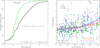 |
Fig. 10 Left : cumulative distributions of NaI D EW divided into two bins according to local SFR: SNe in high and low SFR regions are shown in black and green, respectively. Right : NaI D EW vs local SFR (log scale). Local environments of spiral and elliptical galaxies are shown in blue stars and green crosses, respectively. The red dashed line is the median, the purple is a power-law fit, and the orange is a power-law from a symbolic regression (see Sect. 4.2). |
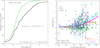 |
Fig. 11 Left : cumulative distributions of NaI D EW divided into two bins according to local stellar mass: SNe in high and low stellar mass regions are shown in black and green, respectively. Right : NaI DEW vs local stellar mass (log scale). Local environments of spiral and elliptical galaxies are shown in blue stars and green crosses, respectively. The red dashed line is the rolling median, the purple is a power-law fit, and the orange is a power-law from a symbolic regression (see Sect. 4.2). |
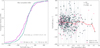 |
Fig. 12 Left: cumulative distributions of NaI D VEL divided into two bins according to normalised offset from the galaxy centre: SNe with high and low offset are shown in purple and blue, respectively. Right: NaI D VEL vs. normalised offset. The red dashed line is the median. |
Significant K-S statistics and correlations for the EW and VEL of narrow lines (other than NaI D ) divided according to galaxy properties.
4.2 Importance of each galaxy parameter
As shown in the K-S tests of Table 4, several galactic parameters strongly influence the NaI D EW. The causality of each of these variables in the column density of the ISM gas is difficult to trace as many galaxy properties are actually correlated with each other; for example, star-forming environments that are more massive are simultaneously more metal-rich, have more dust content, and form stars more actively than less massive ones. We perform several statistical and machine learning tests on our dataset to infer the driving galactic properties and to what extent they can predict the EW.
-
Key driver analysis: We use a key driver analysis (KDA; Tonidandel & LeBreton 2015)11 which quantifies the relative importance of a set of variables, here the environmental properties, in predicting a target quantity, in this case the EW of NaI D . The results are shown in Table 7 for three cases: all galactic properties, only local properties, and only global properties. We show the five most relevant properties in each case. As expected, local properties, particularly the normalised offset and the local star formation rate, are generally more important, although the galaxy T-type plays a substantial role in the EW. It is interesting to note that the absolute score of the KDA given by R2, i.e. the proportion of variance explained, using both local and global information, is still substantially better than using only local information. This means there is some information in the galaxy T-type (third most important) and the galaxy inclination (sixth most important) that is not present uniquely in the local properties inferred in this study. Additionally, it is worth mentioning that even the highest R2 score (0.36) is far from the optimal fully predictable scenario, meaning that it is difficult to recover the EW solely from the properties considered here. To compare, the following six most relevant features according to a gradient-boosting tree algorithm confirm our KDA findings:
 ,
,  ,
,  , T-type,
  and
and  .
.As for the velocity of NaI D , we find a low R2 of 0.073 driven mainly by inclination (26%), normalised offset (23%) and global dust (13%). According to the KDA, the EW contributes less than 10% in importance to the VEL.
Symbolic regression: Symbolic Regression (see e.g. Angelis et al. 2023) is a machine learning tool to find a mathematical expression relating input features, here the galaxy properties that optimise the prediction of a target, here the EW of NaI D , with the least possible mathematical complexity. The algorithm12 searches for combinations of mathematical operators (e.g. addition, +, or power, ^), analytical functions (e.g. cos or log) and constants relating the input galaxy properties to minimise a loss function: LOSS= w(EWpred - EWobs)2, with the weights given by:
 . We find that all the recovered expressions have an RMS larger than 0.7 Å, showing that it is difficult to accurately predict the full diversity of NaI D EW from our galactic properties. On the other hand, the equation with the best score is only dependent on the normalised offset and is an exponential decreasing relation as expected for a typical ISM radial distribution (see previous section): EW(r) = exp (-r/0.31) (see orange line in Figure 8) with a larger ISM scale length than when doing a fit, and larger than the disc scale length, as found in Casasola et al. (2017). If we remove the offset from the input properties, we recover a power-law relation with SFR, i.e. eW=SFRy with γ = 0.10, shown in Figure 10. Similarly, after removing both offset and SFR, we find a power-law relation with log stellar mass, EW= (log M*)0.5 - 3.6 shown in orange in Figure 11. Thus, we confirm with symbolic regression all trends found in the literature and that we previously fitted, although the relations are shallower, as can be seen in the orange lines of the Figures. Regressions relating the EW to a combination of more of these parameters are not preferred by the algorithm.
Regarding the VEL prediction with Symbolic Regression, we find that it is even more difficult to obtain than the EW. The heterogeneous equations involve different variables such as the normalised offset, the local SFR or age, but the RMS is larger than 150 km/s, making any prediction very unreliable.
Key driver analysis of the relative importance of galaxy properties for the NaI D EW.
4.3 Non-ISM contamination
It has been previously reported that the narrow absorption lines of SNe can be related to the intrinsic properties of the explosions and their progenitors. Evolving NaI D lines in SN Ia spectra are associated with CSM (e.g. Ferretti et al. 2016) or to the interaction of the SN radiation with very nearby ISM (e.g. Hoang et al. 2019). In either case, the EW measurement will be dependent on the SN and thus not a trustworthy tracer of the ISM. Other lines, such as KI or even DIBs, have also shown evolution during SN lifetimes (Graham et al. 2015; Milisavljevic et al. 2014). Although statistically, the evolution of intervening SN lines in our sample seems rather absent (see Paper I), the strength of the EW could be affected by SN-interacted nearby material. Phillips et al. (2013) and Maguire et al. (2013) find that there is an excess absorption for possible candidates of SNe with CSM. Regarding the velocity, blueshifted emission lines have been used as indicators of expelled material from the progenitor in various SNe, notably in interacting SNe (e.g. Fransson et al. 2002) but also in narrow absorption lines of SNe Ia (e.g. Sternberg et al. 2013). This material could potentially influence conclusions on galactic gas outflows if it is present.
Moreover, most of the relations found here are heavily driven by SNe Ia, which appear in larger numbers than core-collapse (CC) SNe but, more importantly, occur in a variety of environments and are thus more representative of the ISM extent. To test for possible biases from the SN type, we divide the sample into two different main groups, SNe Ia and CC SNe, and repeat the study carried out for the full sample. We recover the trends with galaxy properties (although with fewer statistics and less significant p-values), as shown in Table 8. However, we also find variations among the different types, notably for the age: SNe Ia show strong differences in EW when dividing the sample into age populations, and CC SNe do not. This is most likely due to the fact that SNe Ia span a much wider range of ages (~Gyr) than CC SNe (~Myr), and in the simple SFH treatment of Equation (6), subtle age differences are less evident. Other smaller variations, as for the inclination, can be explained as SNe Ia include elliptical galaxies where orientation plays a weaker role. The findings divided by each SN type, and the implications for progenitors will be investigated further in a forthcoming study. The unequivocal galaxy trends found in this work clearly show that SN narrow lines are statistically robust tracers of the local ISM, but care should be taken with small samples.
5 Conclusions
We conducted the first statistical study of ISM properties using the narrow absorption lines in SN spectra. With the advantage of being bright and occurring in many environments, SNe are probes of individual sight lines and, consequently, of very local ISM properties. Most notably, with the strength of the EW of NaI D we confirm the literature findings of relations between gas abundance and the distance from the galaxy centre, and with local (0.5 kpc) properties such as the star formation rate, the stellar mass, the dust attenuation, and the stellar age. We also recover the dependence of the gas abundance with global properties such as the galaxy T-type and the inclination of the galaxy.
According to our statistical K-S tests and machine learning approaches, the most important parameters determining the NaI D EW are the normalised offset from the galaxy centre, the local star formation rate and the local stellar mass. However, the other parameters also contribute to the diversity of values. We find, both by fitting and through a symbolic regression, that the EW a) decreases exponentially with the distance from the galactic centre and b) increases as a power-law with the star formation rate and the stellar mass of the local environment. These findings agree well with previous studies based on other ISM tracers.
We conclude that narrow absorption lines within SN spectra are appropriate for statistically investigating the ISM properties of galaxies. At the same time, in a companion paper, we show that they also trace very nearby material in the immediate vicinity of the explosion, contaminating the results of individual events or of smaller samples. In the future, with more statistics, it will be possible to increase the S/N by stacking spectra of different SNe per environmental bin, similarly to galaxy spectra, to obtain more accurate results.
K-S statistics and correlations for the EW of Na I Ddivided according to representative galaxy properties for only SNe Ia and only CC SNe.
Acknowledgements
We thank the anonymous referee for the comments and suggestions that have helped us to improve the paper. S.G.G thanks FCT for financial support through Project No. UIDB/00099/2020 and for support from the ESO Scientific Visitor Programme. C.P.G. acknowledges financial support from the Secretary of Universities and Research (Government of Catalonia) and by the Horizon 2020 Research and Innovation Programme of the European Union under the Marie Skłodowska-Curie and the Beatriu de Pinós 2021 BP 00168 programme, C.P.G. and L.G. recognise the support from the Spanish Ministerio de Ciencia e Innovaciôn (MCIN) and the Agencia Estatal de Investigación (AEI) 10.13039/501100011033 under the PID2023-151307NB-I00 SNNEXT project, from Centro Superior de Investigaciones Cientificas (CSIC) under the PIE project 20215AT016 and the program Unidad de Excelencia Maria de Maeztu CEX2020-001058-M, and from the Departament de Recerca i Universitats de la Generalitat de Catalunya through the 2021-SGR-01270 grant. A.M.G. acknowledges financial support from grant PID2023-152609OA-I00, funded by the Spanish Ministerio de Ciencia, Innovación y Universidades (MICIU), the Agencia Estatal de Investigación (AEI, 10.13039/501100011033), and the European Union’s European Regional Development Fund (ERDF). S.M. acknowledges support from the Research Council of Finland project 350458. This research has made use of the python packages hostphot (Müller-Bravo & Galbany 2022) for galaxy photometry and prospector (Johnson et al. 2021; Leja et al. 2017) for SED fitting. hostphot uses astropy (Astropy Collaboration 2013, 2018, 2022), photutils (Bradley et al. 2023), sep (Barbary 2016; Bertin & Arnouts 1996), ASTROQUERY (Ginsburg et al. 2019), REPROject, extinction (Barbary 2016), sfdmap, pyvo (Graham et al. 2014), ipywidgets and ipympl6. prospector also requires FSPS (Conroy et al. 2009; Conroy & Gunn 2010), PYTHON-FSPS (Johnson et al. 2023) and EMCEE (Foreman-Mackey et al. 2013). We also made use of: numpy (Harris et al. 2020), matplotlib (Hunter 2007), s cipy (Virtanen et al. 2020) and pandas (The pandas development team 2020; Wes McKinney 2010). We use the python implementations of KDA: key-driver-analysis (https://github.com/ bnriiitb/key-driver-analysis) and symbolic regression: PySR (Cranmer 2023) (https://github.com/MilesCranmer/PySR). Computations were performed at the cluster COIN, the CosmoStatistics Initiative, whose purchase was made possible due to a CNRS MOMENTUM 2018-2020 under the project “Active Learning for large scale sky surveys”. This research has made use of the NASA/IPAC Extragalactic Database (NED), which is funded by the National Aeronautics and Space Administration and operated by the California Institute of Technology. This project used public archival data from the Dark Energy Survey (DES), the Sloan Digital Sky Survey (SDSS), the NASA Galaxy Evolution Explorer (GALEX), the Two Micron All Sky Survey (2MASS), the Visible and Infrared Survey Telescope for Astronomy (VISTA). Funding for the SDSS-V has been provided by the Alfred P. Sloan Foundation, the Heising-Simons Foundation, the National Science Foundation, and the Participating Institutions. SDSS acknowledges support and resources from the Center for High-Performance Computing at the University of Utah. SDSS telescopes are located at Apache Point Observatory, funded by the Astrophysical Research Consortium and operated by New Mexico State University, and at Las Campanas Observatory, operated by the Carnegie Institution for Science. The SDSS web site is www.sdss.org. SDSS is managed by the Astrophysical Research Consortium for the Participating Institutions of the SDSS Collaboration, including Caltech, The Carnegie Institution for Science, Chilean National Time Allocation Committee (CNTAC) ratified researchers, The Flatiron Institute, the Gotham Participation Group, Harvard University, Heidelberg University, The Johns Hopkins University, L’Ecole polytechnique fédérale de Lausanne (EPFL), Leibniz-Institut für Astrophysik Potsdam (AIP), Max-Planck-Institut für Astronomie (MPIA Heidelberg), Max-Planck-Institut für Extraterrestrische Physik (MPE), Nanjing University, National Astronomical Observatories of China (NAOC), New Mexico State University, The Ohio State University, Pennsylvania State University, Smithsonian Astrophysical Observatory, Space Telescope Science Institute (STScI), the Stellar Astrophysics Participation Group, Universidad Nacional Autónoma de México, University of Arizona, University of Colorado Boulder, University of Illinois at Urbana-Champaign, University of Toronto, University of Utah, University of Virginia, Yale University, and Yunnan University. Funding for the DES Projects has been provided by the U.S. Department of Energy, the U.S. National Science Foundation, the Ministry of Science and Education of Spain, the Science and Technology Facilities Council of the United Kingdom, the Higher Education Funding Council for England, the National Center for Supercomputing Applications at the University of Illinois at Urbana-Champaign, the Kavli Institute of Cosmological Physics at the University of Chicago, the Center for Cosmology and Astro-Particle Physics at the Ohio State University, the Mitchell Institute for Fundamental Physics and Astronomy at Texas A&M University, Financiadora de Estudos e Projetos, Fundação Carlos Chagas Filho de Amparo à Pesquisa do Estado do Rio de Janeiro, Conselho Nacional de Desen-volvimento Cientifíco e Tecnológico and the Ministério da Ciência, Tecnolo-gia e Inovação, the Deutsche Forschungsgemeinschaft, and the Collaborating Institutions in the Dark Energy Survey. The Collaborating Institutions are
Argonne National Laboratory, the University of California at Santa Cruz, the University of Cambridge, Centro de Investigaciones Energéticas, Medioambi-entales y Tecnológicas-Madrid, the University of Chicago, University College London, the DES-Brazil Consortium, the University of Edinburgh, the Eidgenössische Technische Hochschule (ETH) Zürich, Fermi National Accelerator Laboratory, the University of Illinois at Urbana-Champaign, the Institut de Cièn-cies de l’Espai (IEEC/CSIC), the Institut de Física d’Altes Energies, Lawrence Berkeley National Laboratory, the Ludwig-Maximilians Universität München and the associated Excellence Cluster Universe, the University of Michigan, the National Optical Astronomy Observatory, the University of Nottingham, The Ohio State University, the OzDES Membership Consortium, the University of Pennsylvania, the University of Portsmouth, SLAC National Accelerator Laboratory, Stanford University, the University of Sussex, and Texas A&M University. Based in part on observations at Cerro Tololo Inter-American Observatory, National Optical Astronomy Observatory, which is operated by the Association of Universities for Research in Astronomy (AURA) under a cooperative agreement with the National Science Foundation. The Pan-STARRS1 Surveys (PS1) and the PS1 public science archive have been made possible through contributions by the Institute for Astronomy, the University of Hawaii, the PanSTARRS Project Office, the Max-Planck Society and its participating institutes, the Max Planck Institute for Astronomy, Heidelberg and the Max Planck Institute for Extraterrestrial Physics, Garching, The Johns Hopkins University, Durham University, the University of Edinburgh, the Queen’s University Belfast, the Harvard-Smithsonian Center for Astrophysics, the Las Cumbres Observatory Global Telescope Network Incorporated, the National Central University of Taiwan, the Space Telescope Science Institute, the National Aeronautics and Space Administration under Grant No. NNX08AR22G issued through the Planetary Science Division of the NASA Science Mission Directorate, the National Science Foundation Grant No. AST-1238877, the University of Maryland, Eotvos Lorand University (ELTE), the Los Alamos National Laboratory, and the Gordon and Betty Moore Foundation. GALEX is operated for NASA by the California Institute of Technology under NASA contract NAS5-98034. 2MASS, which is a joint project of the University of Massachusetts and the Infrared Processing and Analysis Center/California Institute of Technology, funded by the National Aeronautics and Space Administration and the National Science Foundation. Based on data products created from observations collected at the European Organisation for Astronomical Research in the Southern Hemisphere under ESO programme 179.A-2010 and made use of data from the VISTA Hemisphere survey (McMahon et al. 2013) with data pipeline processing with the VISTA Data Flow System (Irwin et al. 2004; Lewis et al. 2010; Cross et al. 2012). This work has made use of data from the European Space Agency (ESA) mission Gaia (https://www.cosmos.esa.int/gaia), processed by the Gaia Data Processing and Analysis Consortium (DPAC, https://www.cosmos.esa.int/web/gaia/dpac/consortium). Funding for the DPAC has been provided by national institutions, in particular, the institutions participating in the Gaia Multilateral Agreement.
Appendix A Relation among different lines
Median and median absolute deviations of EW and VEL distributions for various lines.
In this section, we compare the EW and VEL measured from different narrow lines in SN spectra. We consider the following lines: NaID, CaIIH & K, KI 1 & 2, and DIBs 5780, 4428 and 6283. An example of the relation between NaI D and DIB-5780 is shown in Figure A.1 including a Markov chain Monte Carlo (MCMC) linear fit to the data that includes both errors in x and y (Kelly 2007). Despite the high dispersion and weak correlation (ρ = 0.30), these two tracers have a significantly positive EW slope (0.126 ± 0.015). As can be seen for these two lines but also in the comparison with other lines, the sodium lines are stronger and more distinguishable than the rest, especially with low-resolution spectra. Nonetheless, other lines such as the DIB-5780 appear quite clearly in SNe with high extinction. Table A.1 confirms that the median EW values are largest for the NaI D lines.
The correlation between every pair of lines for both EW and VEL is shown in Figure A.2. It can be seen that the correlation between the EW lines is generally weak and for the VEL it is rather absent. The negative correlations in EW are driven by low-number statistics whereas the linear fits for these cases give significantly positive slopes. It is interesting that the EW slopes between potassium lines and DIBs are close to one while they differ with lines of ionised calcium and sodium, in agreement with previous findings (Galazutdinov et al. 2004).
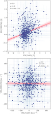 |
Fig. A.1 Comparison of NaI D lines with DIB-5780 for EW (top) and VEL (bottom). The median linear fit is shown in red while in pink are various realisations of the MCMC. The correlation is ρ = 0.30 for the EW and ρ = −0.01 for the VEL, while the median slope is |


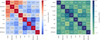 |
Fig. A.2 Spearman correlation coefficients for the EW (left) and the VEL (right) of various combinations of ISM tracers in SN spectra. |
Appendix B Relation between EW and VEL
We present here the relation between EW and VEL of the narrow lines. In Figure B.1 we show the case of Nai D . The VEL values are spread across ±500 km/s around zero and there is no correlation with EW (ρ = 0.07). A linear fit to the data results in a slope of −0.08 ± 5.8, fully consistent with zero. Obtaining accurate velocity measurements when the line is weak or absent is very difficult or impossible. This is reflected in the large VEL dispersion seen at values between ±0.3Å. Therefore, we do not take SNe in this region into account when doing tests of VEL with galaxy properties in section 3. For the other lines, which are weaker, this cut eliminates a higher fraction of SNe. We confirm that we do not find any strong relation between EW and VEL for any of the ISM tracers considered here.
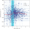 |
Fig. B.1 Comparison of NaI D EW and VEL. The red line portrays the rolling median and the vertical cyan region between ±0.3Å represents the values for which the line is very weak and the uncertainty in VEL is rather large. |
Appendix C Robustness of the K-S tests
The K-S tests performed in this study are very dependent on the location of the split of the two samples being compared. Although in Section 3 we do a sweep changing the split between 40% and 60% of the distribution, and perform a bootstrap simulation, here we do some additional tests. For the global sample, we also take the median split of the MPA/JHU sample (see Figure 7), which lies outside the 40-60% of our sample and find consistent results for the global mass but somewhat lower p-values for SFR (p = 0.035, P = 43%) and sSFR (p = 0.10, P = 24%). Moreover, in Table C.1, we perform K-S tests comparing the EW of the lower and upper quartiles of each galaxy parameter distribution. We confirm all the significant p-values found in Table 4 and also slightly more significant p-values for SFR and sSFR. Finally, although no significant p-values were found for the same sample using the MW lines, we also consider here the look-elsewhere effect (LEE), in which the probability of finding significant differences between populations increases with the number of multiple parameters searched in a given dataset (Miller 1981). The LEE can be compensated by testing each individual hypothesis at a significance corrected by the number of parameters tested (Bonferroni 1936). So, in Table C.1, we include an extra column to the right, in which we recalculate the probabilities of Table 4 for a limiting p-value now of 0.05/N = 0.005, where N = 10 is the number of parameters searched: normalised offset, T-type, inclination and the seven stellar/dust parameters from SED fits (local or global). We leave out other highly correlated parameters (e.g. angular offset). We find that the probabilities still provide significantly high values for all parameters except for the dust index and the local age.
Appendix D Semi-major axes
We compare here the semi-major axes obtained from the homogenised NED database and those extracted from the Kron apertures of hostphot. Figure D.1 shows that the NED values are at least twice as high (with a slope of 0.42 or a median ratio difference of 0.44). This explains why in Figure 8, the range of normalised offsets is mostly below 1, i.e. at smaller distances than the semi-major axis, whereas other studies show the normalised offset or DLR for SNe below and above 1 (e.g. Toy et al. 2025). Since our results are more significant when using NED values (both for offset and inclination), perhaps due to an increased number of objects, we focus our work on the normalisation with NED semi-major axes.
K-S quartile statistics for NaI D EW divided according to galaxy properties.
 |
Fig. D.1 Comparison of semi-major axes from NED and HOSTPHOT. The black dashed line is a 1:1 relation, whereas the red dot-dashed line shows a fit between the two. |
References
- Abbott, T. M. C., Abdalla, F. B., Allam, S., et al. 2018, ApJS, 239, 18 [Google Scholar]
- Abbott, T. M. C., Adamów, M., Aguena, M., et al. 2021, ApJS, 255, 20 [NASA ADS] [CrossRef] [Google Scholar]
- Abdurro’uf, Accetta, K., Aerts, C., et al. 2022, ApJS, 259, 35 [NASA ADS] [CrossRef] [Google Scholar]
- Anderson, T. W., & Darling, D. A. 1952, Ann. Math. Stat., 23, 193 [Google Scholar]
- Angelis, D., Sofos, F., & Karakasidis, T. E. 2023, Archives Comput. Methods Eng., 30, 3845 [Google Scholar]
- Astropy Collaboration (Robitaille, T. P., et al.) 2013, A&A, 558, A33 [NASA ADS] [CrossRef] [EDP Sciences] [Google Scholar]
- Astropy Collaboration (Price-Whelan, A. M., et al.) 2018, AJ, 156, 123 [Google Scholar]
- Astropy Collaboration (Price-Whelan, A. M., et al.) 2022, ApJ, 935, 167 [NASA ADS] [CrossRef] [Google Scholar]
- Barbary, K. 2016, https://doi.org/10.5281/zenodo.804967 [Google Scholar]
- Barbary, K. 2016, J. Open Source Softw., 1, 58 [Google Scholar]
- Barbon, R., Buondi, V., Cappellaro, E., & Turatto, M. 2010, A&AS, 139, 531 [Google Scholar]
- Bell, E. F., & de Jong, R. S. 2001, ApJ, 550, 212 [Google Scholar]
- Bertin, E., & Arnouts, S. 1996, A&AS, 117, 393 [NASA ADS] [CrossRef] [EDP Sciences] [Google Scholar]
- Bianchi, S. 2007, A&A, 471, 765 [NASA ADS] [CrossRef] [EDP Sciences] [Google Scholar]
- Bianchi, L., Conti, A., & Shiao, B. 2014, Adv. Space Res., 53, 900 [Google Scholar]
- Blondin, S., Prieto, J. L., Patat, F., et al. 2009, ApJ, 693, 207 [CrossRef] [Google Scholar]
- Boissé, P., Bergeron, J., Prochaska, J. X., Péroux, C., & York, D. G. 2015, A&A, 581, A109 [NASA ADS] [CrossRef] [EDP Sciences] [Google Scholar]
- Bonferroni, C. 1936, Teoria statistica delle classi e calcolo delle probabilità, Pub-blicazioni del R. Istituto superiore di scienze economiche e commerciali di Firenze (Seeber) [Google Scholar]
- Boquien, M., Buat, V., & Perret, V. 2014, A&A, 571, A72 [NASA ADS] [CrossRef] [EDP Sciences] [Google Scholar]
- Bottinelli, L., Gouguenheim, L., Paturel, G., & de Vaucouleurs, G. 1983, A&A, 118, 4 [NASA ADS] [Google Scholar]
- Bradley, L., Sipocz, B., Robitaille, T., et al. 2023, https://doi.org/10.5281/zenodo.7946442 [Google Scholar]
- Bresolin, F. 2019, MNRAS, 488, 3826 [NASA ADS] [Google Scholar]
- Brinchmann, J., Charlot, S., White, S. D. M., et al. 2004, MNRAS, 351, 1151 [Google Scholar]
- Brout, D., & Scolnic, D. 2021, ApJ, 909, 26 [NASA ADS] [CrossRef] [Google Scholar]
- Bulla, M., Goobar, A., & Dhawan, S. 2018, MNRAS, 479, 3663 [Google Scholar]
- Byrne, R. A., Fraser, M., Cai, Y. Z., Reguitti, A., & Valerin, G. 2023, MNRAS, 524, 2978 [NASA ADS] [CrossRef] [Google Scholar]
- Calzetti, D., Armus, L., Bohlin, R. C., et al. 2000, ApJ, 533, 682 [NASA ADS] [CrossRef] [Google Scholar]
- Casasola, V., Cassarà, L. P., Bianchi, S., et al. 2017, A&A, 605, A18 [NASA ADS] [CrossRef] [EDP Sciences] [Google Scholar]
- Cazzoli, S., Hermosa Munoz, L., Márquez, I., et al. 2022, A&A, 664, A135 [NASA ADS] [CrossRef] [EDP Sciences] [Google Scholar]
- Chen, Y.-M., Tremonti, C. A., Heckman, T. M., et al. 2010, AJ, 140, 445 [Google Scholar]
- Chevalier, R. A., & Fransson, C. 1994, ApJ, 420, 268 [NASA ADS] [CrossRef] [Google Scholar]
- Chevance, M., Kruijssen, J. M. D., Hygate, A. P. S., et al. 2020, MNRAS, 493, 2872 [NASA ADS] [CrossRef] [Google Scholar]
- Choi, J., Dotter, A., Conroy, C., et al. 2016, ApJ, 823, 102 [Google Scholar]
- Chugai, N. N., & Danziger, I. J. 1994, MNRAS, 268, 173 [NASA ADS] [Google Scholar]
- Clark, P., Maguire, K., Bulla, M., et al. 2021, MNRAS, 507, 4367 [NASA ADS] [CrossRef] [Google Scholar]
- Conroy, C., & Gunn, J. E. 2010, ApJ, 712, 833 [Google Scholar]
- Conroy, C., Gunn, J. E., & White, M. 2009, ApJ, 699, 486 [Google Scholar]
- Cranmer, M. 2023, arXiv e-prints [arXiv:2305.01582] [Google Scholar]
- Cross, N. J. G., Collins, R. S., Mann, R. G., et al. 2012, A&A, 548, A119 [NASA ADS] [CrossRef] [EDP Sciences] [Google Scholar]
- Davies, J. I., Nersesian, A., Baes, M., et al. 2019, A&A, 626, A63 [NASA ADS] [CrossRef] [EDP Sciences] [Google Scholar]
- de Vaucouleurs, G. 1959, Handbuch der Physik, 53, 275 [Google Scholar]
- Dessart, L., Gutiérrez, C. P., Kuncarayakti, H., Fox, O. D., & Filippenko, A. V. 2023, A&A, 675, A33 [NASA ADS] [CrossRef] [EDP Sciences] [Google Scholar]
- Dotter, A. 2016, ApJS, 222, 8 [Google Scholar]
- Draine, B. T. 2011, Physics of the Interstellar and Intergalactic Medium (Princeton: Princeton University Press) [Google Scholar]
- Duarte, J., González-Gaitán, S., Mourão, A., et al. 2023, A&A, 680, A56 [NASA ADS] [CrossRef] [EDP Sciences] [Google Scholar]
- Duarte, J., González-Gaitán, S., Mourão, A., et al. 2025, A&A, in press, https://doi.org/10.1051/0004-6361/202554405 [Google Scholar]
- Easeman, B., Schady, P., Wuyts, S., & Yates, R. M. 2022, MNRAS, 511, 371 [NASA ADS] [CrossRef] [Google Scholar]
- Falcón-Barroso, J., Sánchez-Blázquez, P., Vazdekis, A., et al. 2011, A&A, 532, A95 [Google Scholar]
- Fathi, K., Allen, M., Boch, T., Hatziminaoglou, E., & Peletier, R. F. 2010, MNRAS, 406, 1595 [NASA ADS] [Google Scholar]
- Feldmann, R. 2020, Commun. Phys., 3, 226 [NASA ADS] [CrossRef] [Google Scholar]
- Ferretti, R., Amanullah, R., Goobar, A., et al. 2016, A&A, 592, A40 [NASA ADS] [CrossRef] [EDP Sciences] [Google Scholar]
- Ferretti, R., Amanullah, R., Goobar, A., et al. 2017, A&A, 606, A111 [NASA ADS] [CrossRef] [EDP Sciences] [Google Scholar]
- Fielding, D. B., & Bryan, G. L. 2022, ApJ, 924, 82 [NASA ADS] [CrossRef] [Google Scholar]
- Flaugher, B., Diehl, H. T., Honscheid, K., et al. 2015, AJ, 150, 150 [Google Scholar]
- Flewelling, H. A., Magnier, E. A., Chambers, K. C., et al. 2020, ApJS, 251, 7 [NASA ADS] [CrossRef] [Google Scholar]
- Foreman-Mackey, D., Hogg, D. W., Lang, D., & Goodman, J. 2013, PASP, 125, 306 [Google Scholar]
- Förster, F., González-Gaitán, S., Folatelli, G., & Morrell, N. 2013, ApJ, 772, 19 [CrossRef] [Google Scholar]
- Fouque, P., Bottinelli, L., Gouguenheim, L., & Paturel, G. 1990, ApJ, 349, 1 [CrossRef] [Google Scholar]
- Fransson, C., Chevalier, R. A., Filippenko, A. V., et al. 2002, ApJ, 572, 350 [NASA ADS] [CrossRef] [Google Scholar]
- Fraser-McKelvie, A., Cortese, L., Groves, B., et al. 2022, MNRAS, 510, 320 [Google Scholar]
- Frerking, M. A., Langer, W. D., & Wilson, R. W. 1982, ApJ, 262, 590 [Google Scholar]
- Gagliano, A., Narayan, G., Engel, A., Carrasco Kind, M., & LSST Dark Energy Science Collaboration 2021, ApJ, 908, 170 [NASA ADS] [CrossRef] [Google Scholar]
- Gaia Collaboration (Prusti, T., et al.) 2016, A&A, 595, A1 [NASA ADS] [CrossRef] [EDP Sciences] [Google Scholar]
- Gaia Collaboration (Vallenari, A., et al.) 2023, A&A, 674, A1 [NASA ADS] [CrossRef] [EDP Sciences] [Google Scholar]
- Galazutdinov, G. A., Manicò, G., Pirronello, V., & Krełowski, J. 2004, MNRAS, 355, 169 [NASA ADS] [CrossRef] [Google Scholar]
- Gallazzi, A., Charlot, S., Brinchmann, J., White, S. D. M., & Tremonti, C. A. 2005, MNRAS, 362, 41 [Google Scholar]
- Garn, T., & Best, P. N. 2010, MNRAS, 409, 421 [Google Scholar]
- Ginsburg, A., Sipócz, B. M., Brasseur, C. E., et al. 2019, AJ, 157, 98 [NASA ADS] [CrossRef] [Google Scholar]
- González-Gaitán, S., de Jaeger, T., Galbany, L., et al. 2021, MNRAS, 508, 4656 [CrossRef] [Google Scholar]
- González-Gaitán, S., Gutiérrez, C. P., Anderson, J. P., et al. 2024, A&A, 687, A108 [NASA ADS] [CrossRef] [EDP Sciences] [Google Scholar]
- Goodwin, S. P., Gribbin, J., & Hendry, M. A. 1998, The Observatory, 118, 201 [NASA ADS] [Google Scholar]
- Graham, M., Plante, R., Tody, D., & Fitzpatrick, M. 2014, Astrophysics Source Code Library [record ascl:1402.004] [Google Scholar]
- Graham, M. L., Valenti, S., Fulton, B. J., et al. 2015, ApJ, 801, 136 [Google Scholar]
- Gupta, R. R., Kuhlmann, S., Kovacs, E., et al. 2016, AJ, 152, 154 [NASA ADS] [CrossRef] [Google Scholar]
- Gutiérrez, C. P., González-Gaitán, S., Folatelli, G., et al. 2016, A&A, 590, A5 [Google Scholar]
- Gutiérrez, C. P., Anderson, J. P., Hamuy, M., et al. 2017, ApJ, 850, 90 [CrossRef] [Google Scholar]
- Hachinger, S., Röpke, F. K., Mazzali, P. A., et al. 2017, MNRAS, 471, 491 [Google Scholar]
- Harris, C. R., Millman, K. J., van der Walt, S. J., et al. 2020, Nature, 585, 357 [NASA ADS] [CrossRef] [Google Scholar]
- Heidmann, J., Heidmann, N., & de Vaucouleurs, G. 1972, MmRAS, 75, 85 [Google Scholar]
- Ho, L. C., Li, Z.-Y., Barth, A. J., Seigar, M. S., & Peng, C. Y. 2011, ApJS, 197, 21 [Google Scholar]
- Hoang, T., Tram, L. N., Lee, H., & Ahn, S.-H. 2019, Nat. Astron., 3, 766 [Google Scholar]
- Holmberg, E. 1946, Meddelanden fran Lunds Astronomiska Observatorium Serie II, 117, 3 [NASA ADS] [Google Scholar]
- Holmberg, E. 1975, in Galaxies and the Universe, eds. A. Sandage, M. Sandage, & J. Kristian (Chicago: University of Chicago Press), 123 [Google Scholar]
- Hubble, E. P. 1926, ApJ, 64, 321 [Google Scholar]
- Hunter, J. D. 2007, Comp. Sci. Eng., 9, 90 [NASA ADS] [CrossRef] [Google Scholar]
- Irwin, M. J., Lewis, J., Hodgkin, S., et al. 2004, SPIE Conf. Ser., 5493, 411 [Google Scholar]
- Jack, D., & Schröder, K. P. 2019, Rev. Mexicana Astron. Astrofis., 55, 141 [Google Scholar]
- Johnson, B., Foreman-Mackey, D., Sick, J., et al. 2023, https://doi.org/10.5281/zenodo.10026684 [Google Scholar]
- Johnson, B. D., Leja, J., Conroy, C., & Speagle, J. S. 2021, ApJS, 254, 22 [NASA ADS] [CrossRef] [Google Scholar]
- Kacprzak, G. G., Churchill, C. W., Murphy, M. T., & Cooke, J. 2015, MNRAS, 446, 2861 [Google Scholar]
- Kangas, T., Mattila, S., Kankare, E., et al. 2016, MNRAS, 456, 323 [NASA ADS] [CrossRef] [Google Scholar]
- Kauffmann, G., Heckman, T. M., White, S. D. M., et al. 2003, MNRAS, 341, 33 [Google Scholar]
- Kelly, B. C. 2007, ApJ, 665, 1489 [Google Scholar]
- Kolmogorov, A. N. 1933, Giorn Dell’inst Ital Degli Att, 4, 89 [Google Scholar]
- Kron, R. G. 1980, ApJS, 43, 305 [Google Scholar]
- Kroupa, P. 2001, MNRAS, 322, 231 [NASA ADS] [CrossRef] [Google Scholar]
- Lang, D. 2014, AJ, 147, 108 [Google Scholar]
- Leja, J., Johnson, B. D., Conroy, C., van Dokkum, P. G., & Byler, N. 2017, ApJ, 837, 170 [NASA ADS] [CrossRef] [Google Scholar]
- Lewis, J. R., Irwin, M., & Bunclark, P. 2010, ASP Conf. Ser., 434, 91 [Google Scholar]
- Lin, Z., Calzetti, D., Kong, X., et al. 2020, ApJ, 896, 16 [Google Scholar]
- Magnier, E. A., Chambers, K. C., Flewelling, H. A., et al. 2020, ApJS, 251, 3 [NASA ADS] [CrossRef] [Google Scholar]
- Maguire, K., Sullivan, M., Patat, F., et al. 2013, MNRAS, 436, 222 [CrossRef] [Google Scholar]
- Martin, C. L. 2005, ApJ, 621, 227 [NASA ADS] [CrossRef] [Google Scholar]
- McMahon, R. G., Banerji, M., Gonzalez, E., et al. 2013, The Messenger, 154, 35 [NASA ADS] [Google Scholar]
- Meisner, A. M., Lang, D., & Schlegel, D. J. 2017a, AJ, 154, 161 [NASA ADS] [CrossRef] [Google Scholar]
- Meisner, A. M., Lang, D., & Schlegel, D. J. 2017b, AJ, 153, 38 [Google Scholar]
- Milisavljevic, D., Margutti, R., Crabtree, K. N., et al. 2014, ApJ, 782, L5 [Google Scholar]
- Miller, R. G. 1981, Simultaneous Statistical Inference, https://doi.org/10.1007/978-1-4613-8122-8 [Google Scholar]
- Morganson, E., Gruendl, R. A., Menanteau, F., et al. 2018, PASP, 130, 074501 [NASA ADS] [CrossRef] [Google Scholar]
- Morokuma-Matsui, K., & Baba, J. 2015, MNRAS, 454, 3792 [CrossRef] [Google Scholar]
- Morrissey, P., Conrow, T., Barlow, T., et al. 2008, ApJS, 173, 682 [Google Scholar]
- Muñoz-Mateos, J. C., Boissier, S., Gil de Paz, A., et al. 2011, ApJ, 731, 10 [CrossRef] [Google Scholar]
- Müller-Bravo, T., & Galbany, L. 2022, J. Open Source Softw., 7, 4508 [CrossRef] [Google Scholar]
- Namiki, S. V., Koyama, Y., Koyama, S., et al. 2021, ApJ, 918, 68 [Google Scholar]
- Noll, S., Burgarella, D., Giovannoli, E., et al. 2009, A&A, 507, 1793 [NASA ADS] [CrossRef] [EDP Sciences] [Google Scholar]
- Noordermeer, E., & van der Hulst, J. M. 2007, MNRAS, 376, 1480 [Google Scholar]
- Orellana, G., Nagar, N. M., Elbaz, D., et al. 2017, A&A, 602, A68 [NASA ADS] [CrossRef] [EDP Sciences] [Google Scholar]
- Park, J., Jeong, H., & Yi, S. K. 2015, ApJ, 809, 91 [Google Scholar]
- Pascucci, I., Edwards, S., Heyer, M., et al. 2015, ApJ, 814, 14 [Google Scholar]
- Patat, F., Chandra, P., Chevalier, R., et al. 2007, Science, 317, 924 [NASA ADS] [CrossRef] [Google Scholar]
- Paxton, B., Bildsten, L., Dotter, A., et al. 2011, ApJS, 192, 3 [Google Scholar]
- Paxton, B., Cantiello, M., Arras, P., et al. 2013, ApJS, 208, 4 [Google Scholar]
- Paxton, B., Marchant, P., Schwab, J., et al. 2015, ApJS, 220, 15 [Google Scholar]
- Phillips, M. M., et al. 2013, ApJ, 779, 38 [NASA ADS] [CrossRef] [Google Scholar]
- Qin, J., Zheng, X. Z., Fang, M., et al. 2022, MNRAS, 511, 765 [NASA ADS] [CrossRef] [Google Scholar]
- Ritchey, A. M., Welty, D. E., Dahlstrom, J. A., & York, D. G. 2015, ApJ, 799, 197 [NASA ADS] [CrossRef] [Google Scholar]
- Roberts, M. S., & Haynes, M. P. 1994, ARA&A, 32, 115 [NASA ADS] [CrossRef] [Google Scholar]
- Rodríguez, S., & Padilla, N. D. 2013, MNRAS, 434, 2153 [CrossRef] [Google Scholar]
- Rupke, D. S., Veilleux, S., & Sanders, D. B. 2005a, ApJS, 160, 87 [NASA ADS] [CrossRef] [Google Scholar]
- Rupke, D. S., Veilleux, S., & Sanders, D. B. 2005b, ApJS, 160, 115 [Google Scholar]
- Saintonge, A., & Catinella, B. 2022, ARA&A, 60, 319 [NASA ADS] [CrossRef] [Google Scholar]
- Salim, S., Rich, R. M., Charlot, S., et al. 2007, ApJS, 173, 267 [NASA ADS] [CrossRef] [Google Scholar]
- Sánchez-Menguiano, L., Sánchez, S. F., Pérez, I., et al. 2018, A&A, 609, A119 [NASA ADS] [CrossRef] [EDP Sciences] [Google Scholar]
- Scargle, J. D., Norris, J. P., Jackson, B., & Chiang, J. 2013, ApJ, 764, 167 [Google Scholar]
- Simha, V., Weinberg, D. H., Conroy, C., et al. 2014, arXiv e-prints [arXiv:1404.0402] [Google Scholar]
- Simon, J. D., Gal-Yam, A., Gnat, O., et al. 2009, ApJ, 702, 1157 [NASA ADS] [CrossRef] [Google Scholar]
- Skrutskie, M. F., Cutri, R. M., Stiening, R., et al. 2006, AJ, 131, 1163 [NASA ADS] [CrossRef] [Google Scholar]
- Smirnov, N. V. 1939, Bull. Math. Univ. Moscou, 2, 3 [Google Scholar]
- Sollerman, J., Cox, N., Mattila, S., et al. 2005, A&A, 429, 559 [NASA ADS] [CrossRef] [EDP Sciences] [Google Scholar]
- Spearman, C. 1904, Am. J. Psychol., 15, 201 [CrossRef] [Google Scholar]
- Sternberg, A., Gal-Yam, A., Simon, J. D., et al. 2011, Science, 333, 856 [NASA ADS] [CrossRef] [Google Scholar]
- Sternberg, A., Gal Yam, A., Simon, J. D., et al. 2013, arXiv e-prints [arXiv:1311.3645] [Google Scholar]
- Sullivan, M., Le Borgne, D., Pritchet, C. J., et al. 2006, ApJ, 648, 868 [NASA ADS] [CrossRef] [Google Scholar]
- The pandas development team 2020, https://doi.org/10.5281/zenodo.3509134 [Google Scholar]
- Tonidandel, S., & LeBreton, J. 2015, J. Business Psychol., 30, 207 [Google Scholar]
- Toy, M., Wiseman, P., Sullivan, M., et al. 2025, MNRAS, submitted [arXiv:2408.03749] [Google Scholar]
- Tuffs, R. J., Popescu, C. C., Voelk, H. J., Kylafis, N., & Dopita, M. A. 2004, Astron. Nachr. Suppl., 325, 1.118 [Google Scholar]
- Virtanen, P., Gommers, R., Oliphant, T. E., et al. 2020, Nat. Methods, 17, 261 [Google Scholar]
- Walcher, J., Groves, B., Budavári, T., & Dale, D. 2011, Ap&SS, 331, 1 [NASA ADS] [CrossRef] [Google Scholar]
- Waters, C. Z., Magnier, E. A., Price, P. A., et al. 2020, ApJS, 251, 4 [NASA ADS] [CrossRef] [Google Scholar]
- Welty, D. E., Ritchey, A. M., Dahlstrom, J. A., & York, D. G. 2014, ApJ, 792, 106 [Google Scholar]
- Wes McKinney 2010, in Proceedings of the 9th Python in Science Conference, ed. Stéfa [Google Scholar]
- Xu, X., Heckman, T., Yoshida, M., Henry, A., & Ohyama, Y. 2023, ApJ, 956, 142 [Google Scholar]
- Yuan, Q.-r., & Zhu, C.-x. 2004, Chinese Astron. Astrophys., 28, 127 [Google Scholar]
- Yuan, F.-T., Lu, J., Shen, S., & Boquien, M. 2021, ApJ, 911, 145 [NASA ADS] [CrossRef] [Google Scholar]
Using OpenAI, (2025), ChatGPT (Apr version), https://chat.openai.com
They used a Kroupa IMF as in the current work.
We also tried the Anderson-Darling test (Anderson & Darling 1952) with consistent results.
In fact, we do not recover the mass-metallicity relation neither for our local nor global stellar fits.
For the significance of the correlation, we use the same ranges as those presented in Gutiérrez et al. (2017).
Key driver analysis is also referred to as Importance Analysis or Relative Importance Analysis and it uses Johnson’s Relative Weights, a combination of principal component analysis on the predictor variables and least square regression to predict the target quantity.
This is a multi-population evolutionary algorithm which applies behaviours of biological organisms such as reproduction, mutation, and recombination and follows a natural selection process to solve an optimisation problem.
All Tables
K-S statistics and correlations for NaI D EW divided according to galaxy properties.
Significant K-S statistics and correlations for NaIDVEL divided according to galaxy properties.
Significant K-S statistics and correlations for the EW and VEL of narrow lines (other than NaI D ) divided according to galaxy properties.
Key driver analysis of the relative importance of galaxy properties for the NaI D EW.
K-S statistics and correlations for the EW of Na I Ddivided according to representative galaxy properties for only SNe Ia and only CC SNe.
Median and median absolute deviations of EW and VEL distributions for various lines.
All Figures
|
Fig. 1 Galaxy type distribution of our SN sample. n = 985 is the number of SN host galaxies. |
| In the text | |
|
Fig. 2 Sketch of a spiral galaxy3 with the SN (blue star) indicating as a blue line the angular offset with the host centre Δα, in red the semimajor axis a of the ellipse, and in purple the directional light radius dDLR. |
| In the text | |
|
Fig. 3 Representative HOSTPHOT images of SN 2001ed with the filters: FUV (GALEX) and W2 (unWISE). Masked sources are shown in grey, and the global Kron apertures are shown as red ellipses. The galaxy centre is shown as a purple cross, whereas the SN position is a cyan star. |
| In the text | |
|
Fig. 4 Representative HOSTPHOT images of SN 2001el with the filters: zDECam (DES) and JVISTA (VISTA). Masked sources are shown in grey, and the local circular apertures for r = 0.5 kpc are shown as red lines. The cyan star denotes the SN position. We note that the images have different orientations and resolutions. |
| In the text | |
|
Fig. 5 PROSPECTOR SED fits to the observed global photometry of the host galaxy of SN 2010H (left) and local photometry of the host galaxy of SN 2002bf (right). The observed photometry is shown with orange circles with corresponding filter names. The median MCMC fit is shown in dark green with synthetic photometry as green squares, and 100 MCMC realisations are shown in light green. |
| In the text | |
|
Fig. 6 Corner plots resulting from PROSPECTOR SED fits to the observed global/local photometry of the host galaxy of SN 2010H/SN 2002bf (left/right). The six free parameters (logM*, logZ*, τv or dust2, tage, log τ, and dust index n) are shown in each panel. |
| In the text | |
|
Fig. 7 Stellar mass (left), SFR (middle), and sSFR (right) distributions of our sample (blue) compared with the SDSS measurements (grey) from the MPA/JHU catalogue. The vertical dashed lines mark the median values for each distribution. |
| In the text | |
|
Fig. 8 Left : cumulative distributions of NaID EW divided into four bins according to normalised offset. K-S tests indicate that all bins are not drawn from the same distribution. Right: NaI D EW vs normalised offset. SNe located in spirals and ellipticals are highlighted as blue stars and green crosses, respectively. At the top of the figure, n = 667 is the number of events, rS = −0.44 is the Spearman correlation coefficient, and P = 6.3 × 10⁻³³ is the probability of detecting a correlation by chance. The vertical dash-dotted lines represent the 25th, 50th and 75th percentiles of the sample from which the cumulative distributions are obtained. The red dashed line is the rolling median, the purple solid line is the exponential fit to the medians, with the shaded purple area indicating the 1σ uncertainty, and the orange line an exponential function from a symbolic regression (see Sect. 4.2). |
| In the text | |
|
Fig. 9 K-S test p-values (log) of NaID EW divided according to galaxy properties: normalised offset, T-type, inclination, and local stellar and dust properties. |
| In the text | |
|
Fig. 10 Left : cumulative distributions of NaI D EW divided into two bins according to local SFR: SNe in high and low SFR regions are shown in black and green, respectively. Right : NaI D EW vs local SFR (log scale). Local environments of spiral and elliptical galaxies are shown in blue stars and green crosses, respectively. The red dashed line is the median, the purple is a power-law fit, and the orange is a power-law from a symbolic regression (see Sect. 4.2). |
| In the text | |
|
Fig. 11 Left : cumulative distributions of NaI D EW divided into two bins according to local stellar mass: SNe in high and low stellar mass regions are shown in black and green, respectively. Right : NaI DEW vs local stellar mass (log scale). Local environments of spiral and elliptical galaxies are shown in blue stars and green crosses, respectively. The red dashed line is the rolling median, the purple is a power-law fit, and the orange is a power-law from a symbolic regression (see Sect. 4.2). |
| In the text | |
|
Fig. 12 Left: cumulative distributions of NaI D VEL divided into two bins according to normalised offset from the galaxy centre: SNe with high and low offset are shown in purple and blue, respectively. Right: NaI D VEL vs. normalised offset. The red dashed line is the median. |
| In the text | |
|
Fig. A.1 Comparison of NaI D lines with DIB-5780 for EW (top) and VEL (bottom). The median linear fit is shown in red while in pink are various realisations of the MCMC. The correlation is ρ = 0.30 for the EW and ρ = −0.01 for the VEL, while the median slope is |
| In the text | |
|
Fig. A.2 Spearman correlation coefficients for the EW (left) and the VEL (right) of various combinations of ISM tracers in SN spectra. |
| In the text | |
|
Fig. B.1 Comparison of NaI D EW and VEL. The red line portrays the rolling median and the vertical cyan region between ±0.3Å represents the values for which the line is very weak and the uncertainty in VEL is rather large. |
| In the text | |
|
Fig. D.1 Comparison of semi-major axes from NED and HOSTPHOT. The black dashed line is a 1:1 relation, whereas the red dot-dashed line shows a fit between the two. |
| In the text | |
Current usage metrics show cumulative count of Article Views (full-text article views including HTML views, PDF and ePub downloads, according to the available data) and Abstracts Views on Vision4Press platform.
Data correspond to usage on the plateform after 2015. The current usage metrics is available 48-96 hours after online publication and is updated daily on week days.
Initial download of the metrics may take a while.