| Issue |
A&A
Volume 700, August 2025
|
|
|---|---|---|
| Article Number | A142 | |
| Number of page(s) | 18 | |
| Section | Planets, planetary systems, and small bodies | |
| DOI | https://doi.org/10.1051/0004-6361/202554759 | |
| Published online | 19 August 2025 | |
Ultraviolet auroral bridge of Jupiter
The effect of the solar wind on the morphology of the polar aurora
1
Laboratory for Planetary and Atmospheric Physics, University of Liège,
Liège,
Belgium
2
University of Minnesota,
Minneapolis,
MN,
USA
3
Institute for Space Astrophysics and Planetology, National Institute for Astrophysics (INAF-IAPS),
Rome,
Italy
4
Planetary Science Institute,
Tucson,
AZ,
USA
5
LIRA, Observatoire de Paris, Université PSL, Sorbonne Université, Université de Paris Cité, CY Cergy, Paris Université, CNRS,
Meudon
92190,
France
6
Southwest Research Institute,
San Antonio,
TX,
USA
★ Corresponding author: This email address is being protected from spambots. You need JavaScript enabled to view it.
Received:
26
March
2025
Accepted:
2
July
2025
Abstract
The ultraviolet aurora of Jupiter frequently shows a number of arcs between the dusk-side polar region and the main emission. These arcs are called “bridges”. We present a largely automated detection and statistical analysis of the bridges in over 248 Hubble-Space-Telescope observations. We also performed a multi-instrument study of the magnetic field line crossings that are connected to bridges by the Juno spacecraft during its first 30 perijoves. The bridges are observed to arise on timescales of ~2 hours, they can persist over a full Jupiter rotation, and they are conjugate between hemispheres. The appearance of the bridges is associated with the compression of the magnetosphere, likely by the solar wind. Low-altitude bridge crossings are associated with upward-dominated broadband electron distributions, consistent with Zone II aurorae, and also with plasma-wave emission observed by Juno-Waves. This agrees with existing theoretical models for the generation of aurorae in the polar regions. Main-emission crossings in which no bridges are visible also show characteristics that are associated with bridges (a stronger upward electron flux and plasma wave emission), which is not the case for main-emission crossings with visible bridges, as though bridges remain present, but are spatially indistinguishable from the main emission in the former case. In all, the compression of the magnetosphere may work to spatially separate the Zone I and Zone II regions of the main emission in the form of Zone II bridges.
Key words: methods: data analysis / planets and satellites: aurorae / planets and satellites: gaseous planets / planets and satellites: magnetic fields / planets and satellites: individual: Jupiter
© The Authors 2025
 Open Access article, published by EDP Sciences, under the terms of the Creative Commons Attribution License (https://creativecommons.org/licenses/by/4.0), which permits unrestricted use, distribution, and reproduction in any medium, provided the original work is properly cited.
This article is published in open access under the Subscribe to Open model. This email address is being protected from spambots. You need JavaScript enabled to view it. to support open access publication.
1 Introduction
The ultraviolet (UV) aurora of Jupiter is home to a number of distinct and discrete features. Of these, the UV auroral “bridges” (Pardo-Cantos 2019) of Jupiter are one of the largest and are present most consistently, although they have typically been discussed in the context of wider studies of the aurora so far (e.g. Palmaerts et al. 2023; Greathouse et al. 2021; Nichols et al. 2009b), and their underlying processes have not yet been the subject of a dedicated study. We exclusively address the auroral bridge, and we therefore provide details on its observational characteristics, origins, and relation to other features in the jovian aurora.
We refer to any arc-like feature in the auroral polar region of Jupiter as a bridge that spans (though not necessarily fully) the polar collar (Greathouse et al. 2021) between the main auroral emission (ME) of Jupiter (e.g. Grodent et al. 2003) and the day-side active region (Nichols et al. 2017). An example image of the aurora with multiple bridges is shown in Figure 1. These bridges are present within the dusk-side polar collar and connect the ME to the noon active region. This feature has previously been referred to as the “arc-like feature of the polar active region” (Grodent 2015) or “arcs parallel to the main oval” (Nichols et al. 2017). We use the term “bridge” to highlight its bridge-like nature, which is visible between the ME and the polar region, and to distinguish this feature from other arcs in the polar region, such as the polar auroral Filaments (PAFs) (Nichols et al. 2009a).
Thus far, the only dedicated study of the auroral bridge was made by Pardo-Cantos (2019), who analysed three images of the aurora that contained bridges and were taken by the Space Telescope Imaging Spectrograph (STIS) instrument on board the Hubble Space Telescope (HST). In these cases, the bridges were found to map to the dusk-side magnetosphere between 10 and 22 magnetic local time (MLT) and to be largely confined to distances greater than 60 RJ. Based on its approximate mapped position in the magnetosphere, the bridge was suggested to arise from vorticity in the dusk-side plasma flow (Fukazawa et al. 2006) caused by Kelvin-Helmholtz instabilities, but neither Kelvin-Helmholtz instabilities nor dusk-side reconnection (as suggested by e.g. Grodent et al. 2003; Cowley et al. 2003) are individually sufficient to explain the appearance of bridges (Nichols et al. 2017), and the question of their origins remains open.
Greathouse et al. (2021) also observed bridges in Juno Ultra-Violet Spectrograph (Juno-UVS) images of both hemispheres of the aurorae of Jupiter. Because the aurora is not symmetric around the axis of rotation of Jupiter, especially in the northern hemisphere, HST observations are typically made when the largest proportion of the jovian aurora is visible, that is, around System-III subsolar longitudes of 150° in the north and 30° in the south. This introduces a local-time bias. However, as a space-craft in polar orbit around Jupiter, Juno can image the aurora at many subsolar longitudes and can thus remove the local-time bias. Bright, dusk-side concentric arcs (Greathouse et al. 2021) in the polar collar (which we identify as bridges in this work) were observed independently of System-III longitude, indicating that bridges originate in the dusk-side magnetosphere. The emergence of bridges has also been tentatively associated with the solar wind compression of the jovian magnetosphere (Nichols et al. 2007, 2009b, 2017). Nichols et al. (2009b) also indicated that the bridge was stable over at least 3 hours, which was supported by later Juno observations that the two bridges were stable over at least 5 hours (Palmaerts et al. 2023). Based on the typical timescale for solar wind compression events, this suggests that bridges may have lifetimes of several days. Dusk-side polar-collar arcs (identified as bridges) have also been observed to disrupt the smooth morphology of the dusk-side ME on occasion (Groulard et al. 2024), and in other instances, they appeared alongside an unperturbed ME (Nichols et al. 2009b). This may indicate that the process that gives rise to bridges can (but is not required to) interact with the source process of the ME. A correlation between solar wind compression of the magnetosphere and the appearance of dusk-side polar arcs in the aurora was identified in a limited number of cases during the approach of Juno to Jupiter (Nichols et al. 2017).
From particle measurements made by Juno, the auroral region can be split into several zones (Mauk et al. 2020). Of these, Zone I (ZI) and Zone II (ZII), typically associated with the ME, are most relevant to this work. ZI is associated with predominantly planetward- or downward-moving electrons, equivalent to upward field-aligned currents (FACs). ZII is immediately poleward of the ZI subregion and is dominated by upward-moving electrons (downward FACs). ZI and ZII are typically located alongside one another, such that the ME has been associated with an inversion of the FACs, upward and then downward, as Juno crosses the ME into the polar region (Al Saati et al. 2022). Auroral emission in the polar region, particularly the ZII aurora, has been suggested to be the consequence of broadband bidirectional electron acceleration by upward-travelling electrostatic waves (ESWs) (Sulaiman et al. 2022) that are generated by the upward electron beams (Elliott et al. 2018, 2020) observed by Juno (Mauk et al. 2017b). This is noteworthy since analogous processes on Earth and Saturn do not give rise to appreciable auroral emission (Sulaiman et al. 2022).
We investigate the jovian auroral bridge using two methods: firstly, a largely automatic analysis of a large number of HST-STIS images of the aurora to determine the statistical properties of the bridges; and secondly, a multi-instrument analysis of Juno data from the first 30 perijoves to place the bridge in a wider magnetospheric context. The results from these two investigations are then combined to discuss the bridge in the context of existing auroral frameworks.
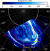 |
Fig. 1 300-second image of the northern jovian UV aurora captured by HST during the GO-15638 campaign (exposure ID: odxc01okq). A 15° × 15° grid in System-III longitude and planetocentric latitude is included; the System-III longitude of certain meridians is given in white, and certain planetocentric latitudes are shown in magenta. The average subsolar longitude during this exposure (170°) is denoted by the solid yellow line, and the positions of the dawn and dusk hemispheres are included for guidance. The approximate location of the polar collar is enclosed by dashed red lines and the location of the noon active region by a dashed green ellipse. The bridges are highlighted with yellow arrows. |
2 Observations
In the first part of this work, we consider HST-STIS UV observations between 2012 and 2023, notably those from the campaigns GO-11649, 12883, 13035, 14105, 14634, 15638, 16193, and 16675. For the automated bridge detection discussed in Section 3.1, we consider only northern hemisphere visits because the viewing geometry in the northern hemisphere is favourable for observation of the dusk-side polar region (where the bridges are located) from an Earth orbit, equivalent to 248 unique HST-STIS visits or 143 hours of observation. These time-tagged images were accumulated into 10-second frames using the CAL-STIS calibration tools from the Space Telescope Science Institute (Katsanis & McGrath 1998), and they were then converted into brightness in kilo-Rayleigh (kR) assuming a colour ratio of 2.5 (Gustin et al. 2012) and were fitted to the ellipsoid of Jupiter following (Bonfond et al. 2009).
Composite UV images from Juno-UVS (68–210 nm; Gladstone et al. 2017) were also used. Juno has a highly elliptical polar orbit, which allows it to view the jovian aurora in both hemispheres. As a spin-stabilised spacecraft, Juno cannot point its instruments freely; instead, Juno-UVS observes strips of the jovian aurora as the spacecraft rotates, which can be collated to create wider maps of the aurora. For each pass of the Juno spacecraft over the poles (a perijove; designated as e.g. PJ1-N for perijove 1, northern hemisphere), an exemplar map was produced from Juno-UVS data. This exemplar map uses a 100-spin (~50-minute) stack of UVS data that was centred as close as possible to the perijove time whilst covering at least 75% of the auroral region (Bonfond et al. 2018). Radiation noise from the impinging of high-energy electrons on the detector was also removed (Bonfond et al. 2021). A detailed description of the production of the exemplar map is given by Head et al. (2024). This resulted in a representative view of the aurora in each hemisphere during each perijove. In total, this corresponded to 58 images of the aurora for the first 30 perijoves, 2 images per perijove excluding PJ2, when Juno was placed in safe mode.
In addition to image data from Juno-UVS, data from other Juno instruments were used, notably from the Flux-Gate Magnetometer (MAG-FGM; Connerney et al. 2017), the Juno Energetic-particle Detector Instrument (JEDI; Mauk et al. 2017a), and the Waves instrument (Kurth et al. 2017). The technical details of each instrument are described within their associated reference.
3 Methods
3.1 Automatic detection of bridge-like arcs
In the first part of this work, we employ an automated method to detect bridge-like arcs in 248 HST-STIS images of the northern aurora. Each STIS time-tag image series was typically split into 30-second frames, which presents a compromise between image noise reduction and preservation of auroral dynamics. These images were first mapped into a polar projection as though they were observed from directly above the rotation axis of Jupiter, with a System-III longitude of 0° at the top of the image and 90° to the right to facilitate the comparison between images whilst preserving the physical size of the features in the aurora. We collated each STIS image series into a single frame by taking the pixelwise median of the image stack; since prior investigations indicated that the bridge morphology does not greatly change over the 40 minutes of a HST exposure (Nichols et al. 2009b), this reduces the required computational effort whilst ensuring that each image represents a unique instance of the auroral morphology. Although bridges have been observed to remain fixed in local time (Pardo-Cantos 2019) rather than in System-III longitude (and thus, they are observed to slowly advance in longitude over the course of a STIS exposure), they remain clearly visible in the collated images, as shown in Figure 1. To highlight the arc-like form of the bridges more clearly, and hence, to make the automatic detection of these structures more feasible, each collated image was convolved with a Gaussian-arc kernel to produce an arcness map of the aurora, as shown in Figure A.1a (see Section 3.2 of Head et al. (2024) for a thorough description of this method).
Bridges are defined as arcs that connect the day-side active region to the ME via the polar collar (although they may not span this gap fully). This implies that they must traverse a significant (>50 RJ) radial distance in the magnetosphere, since the ME is surmised to originate from a region between 20 and 40 RJ from Jupiter (Cowley & Bunce 2001), whereas the active region is firmly within the polar aurora, and it hence maps to more distant regions of the magnetosphere. This behaviour can be leveraged to automatically detect auroral arcs that are likely to be bridges. The details of this method are described in Appendix A.1. Briefly, a number of fixed-radius contours are magnetically mapped from the magnetosphere to the ionosphere, and the locations in which auroral arcs cross these contours are used as starting points to follow the shape of each arc in the ionosphere. Random-forest filtering is used alongside manual bridge-arc designations to remove artefacts from the method. An example of the detected arcs after this filtering is given in Figure 2.
3.2 Juno multi-instrument analysis
In the second part of this work, we combine data from multiple Juno instruments to build a full picture of the bridge. These quantities are determined as follows:
Field-aligned currents were calculated from FGM data compared against the latest JRM33 magnetic field model (Connerney et al. 2022) (implemented using the JupiterMag Python wrapper; James et al. 2022; Wilson et al. 2023) and extrapolated via magnetic flux conservation to the assumed auroral altitude of 400 km following Al Saati et al. (2022); see Section A.2.
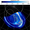
Fig. 2 Results of the bridge-detection algorithm after filtering. The solid red lines denote detected arcs that were identified as bridges. The dashed dark red lines denote arcs that were identified as PAFs. The seed point of each arc is shown in magenta. Manually designated arcs are plotted in green. The white contours delineate the validity region of the Vogt et al. (2011) JRM33 flux-equivalence mapping along closed field lines.
The Alfvénic Poynting flux was determined based on FGM data, extrapolated via magnetic flux conservation to the assumed auroral altitude of 400 km following the method presented by Gershman et al. (2019).
The electron energy and pitch-angle distribution were determined based on JEDI measurements (Mauk et al. 2017a), where data from all detectors were stacked.
The Juno-Waves spectrum was adopted from Juno-Waves data; we only present data from the LFR-Lo channel (50 Hz to 20 kHz).
Non-UVS data were sourced from the Automated Multi-Dataset Analysis (AMDA) database that is maintained by the Centre des Données de la Physique des Plasmas (Génot et al. 2021) and accessed using the speasy Python library (Jeandet & Schulz 2024), with the exception of JEDI data, which were downloaded using the JMIDL tool provided by the John Hopkins University.
We had only a few cases (58 over 30 PJs) and therefore determined the bridge positions in each exemplar image, and hence the Juno bridge traversal timestamps, manually (using the arc-convolved exemplar images, similar to Figure 2a, to highlight the arc locations) to avoid introducing artefacts or omitting bridges by the automatic detection algorithm. The Juno footprint was considered to cross a manually identified arc when within 5 px (~600 km); this is a relatively broad threshold to ensure that the full arc crossing is included. Because the auroral morphology in the base image was determined from stacked UVS spectral scan centred at a particular time, however, it may not be representative of the auroral morphology at the time of a supposed Juno bridge traversal. This effect can be counteracted by employing the instantaneous UVS map of the aurora at the time of the suspected bridge crossing to ensure that the bridge was approximately in the same position as in the exemplar image and adjusting the crossing timestamps if necessary. The mean (and standard deviation) difference between the exemplar-map time and bridge crossings is 44 minutes (±23 minutes), so that most bridge crossings were reliably determined from the initial manual estimates. Additionally, since the auroral arcs of bridges and the ME are typically crossed perpendicularly, the instantaneous UVS Juno-footprint brightness should show a peak during the supposed crossings. This can be used as an additional validity check of the time stamp. We considered the first 30 perijoves because after the 30th orbit, the orbit of Juno is such that incomplete maps of the northern aurora become increasingly common. This makes it difficult to identify mesoscale features such as bridges, and passes over the southern aurora occur at increasingly greater altitudes, which lowers the resolution of the southern auroral maps and again makes the identification of the bridge challenging. Details of the automatically detected bridge and ME crossings are given in Table C.1.
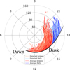 |
Fig. 3 Automatically detected bridge and PAF-like arcs (in pale red and blue) in all northern-hemisphere HST-STIS observations we considered, mapped via flux-equivalence mapping to the magnetospheric equator (radius and local time). The radii are given in RJ. A set of average bridge and PAF contours is given in dark red and blue; their starting locations on the Joy et al. (2002) expanded magnetopause (solar wind ram pressure = 0.039 nPa; stand-off distance 92 RJ) are given in black. |
3.3 HST-STIS large-scale analysis
Detected bridges in the ionosphere were magnetically mapped to the equatorial plane in the magnetosphere using the Vogt et al. (2011) flux-equivalence mapping. Figure 3 shows that the majority of the detected bridges (light red) map to the dusk-side magnetosphere between 10 and 20 MLT, as expected from previous work (Pardo-Cantos 2019). Detected arcs that map to the magnetopause beyond 16 MLT were considered to be PAFs and were excluded from this analysis, to be discussed separately below, although a continuum of arcs exists between bridges and PAFs, and the choice of this cutoff is therefore approximate.
To help us understand the average properties of these bridges, average-bridge contours (dark red, and blue for PAFs in Figure 3) were calculated by taking a number of starting points on the magnetopause (black in Figure 3), following the average orientation of detected bridges (weighted by the inverse square of the distance to the point to produce a local average orientation), and continuing this process to propagate each contour into the magnetosphere. These contours indicate that bridges typically curve duskward and radially inwards toward Jupiter. The bridge mapping shown in Figure 3 depends on the magnetic field model that is used to map poleward of the ME. Although the quantitative details are affected by the choice of this model (compare Figure 3 with Figure B.2 using field-line tracing instead of flux-equivalence mapping), our results are broadly consistent with the expected location of the bridges. The bridges are thus named because they (at least partially) bridge the polar collar between the active region (which can be assumed to relate to the magnetopause or at least to large radial distance in the day-side magnetosphere; Nichols et al. 2007) and the ME (which is expected to arise much closer to Jupiter, at ~30 RJ; Cowley & Bunce 2001).
Of all the HST cases we analysed, only one quasi-continuous set of observations exists (notably, surrounding PJ6) that tracks the evolution of a bridge over a full Jupiter rotation; the start and end series of this set are shown in Figure 4. The bridge has persisted over the ~10 h span of this set of observations with very little change in morphology, besides moving slightly equatorward. This result is consistent with the findings of Palmaerts et al. (2023) and Nichols et al. (2009b), who reported that the bridges were stable over at least 3 hours. The latter work also associated the appearance of bridges with magnetospheric compression by the solar wind, which was noted to be maintained over several days. This is consistent with bridges that can survive a full Jupiter rotation. A case in which a bridge was observed to develop between two HST observations is given in Figure 5 (see the supplementary material for GIF images of these cases). In this case, the ME was observed to first exist as two parallel arcs that had evolved into a clear bridge-like arc separate from the ME one hour later, although this interpretation assumes that the two double-arc phenomena are related. This is impossible to confirm in the absence of intervening observations. In any case, this hour-scale onset is consistent with the suggested solar wind influence on the presence of bridges (Nichols et al. 2017), since it is expected to vary on timescales of hours (Chané et al. 2017). Some internal processes (e.g. dawn storms) are also known to vary over hour timescales, however (Bonfond et al. 2021), and this timescale therefore cannot be used as a confirmation of the influence of the solar wind without further supporting evidence.
The appearance of bridges can also be directly related to the compression of the magnetosphere. Figure 6 shows the expansion of the ME against the total detected bridge count for each northern HST series we considered, where “expansion” refers to the average equatorward distance (in kilometres) of the ME from its average position, according to Head et al. (2024). The use of bridge count over the total projected bridge length in the magnetosphere, for example, may potentially misrepresent the aurora when many small bridges are detected. Figure B.3 shows a broadly linear relation between detected bridge count and the total projected bridge length. We therefore conclude that both parameters are reasonable measures of the quantity of bridges in the aurora. Figure 6 shows no clear relation between the bridge count and the ME expansion. By isolating the cases in which the state of compression of the magnetosphere is known from Juno magnetopause-crossing altitudes (Yao et al. 2022; Louis et al. 2023), however, a clear distinction between cases with compressed and uncompressed magnetospheres is apparent. A Pearson-χ2 test on these points with categories [bridge count > 0, bridge count = 0] and [compressed magnetosphere, uncompressed magnetosphere] indicates that the compression of the magnetosphere is associated with the presence of bridges beyond the 99th percentile level (χ2 = 9.73, p-value 0.002). This association between magnetospheric compression and bridge count is evident even from a cursory inspection of the aurora in these cases, which we show in Figure B.1. While the size of the magnetosphere may vary as a result of a number of factors, such as the solar wind dynamic pressure (Chané et al. 2017) and the mass-outflow rate from Io (Bagenal & Delamere 2011), this result, combined with the previously determined hour-scale variability of bridge morphology, is compatible with the idea that the solar wind exerts some measure of influence on the appearance of bridges in the aurora, which agrees with the results of Nichols et al. (2017). This scenario cannot be robustly confirmed without simultaneous measurement of the solar wind near Jupiter, however, which is left to a future work. The arcs we used in the above analysis were those with magnetopause local times shorter than 16 MLT; these arcs can be confidently said to be bridges, whereas there is some ambiguity with PAFs in the arcs that map to the distant magnetosphere beyond 16 MLT. A similar analysis was performed separately for the assumed PAFs (blue in Figure 3), and no difference was found in the total detected arc length for compressed and uncompressed magnetospheres (see Figure B.4 in the supplementary material). This suggests that PAFs are not exactly the same feature as the auroral bridge and that they do not depend on the solar wind, in agreement with Nichols et al. (2009a). The methods we presented are not necessarily suitable for the analysis of these polar-cap features, which are often found within the region of open magnetic flux according to Vogt et al. (2011), and more specialised work should therefore be carried out to confirm this conclusion.
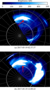 |
Fig. 4 Observation of a persistent bridge-like arc over a full Jupiter rotation in the southern aurora during the GO-14634 HST campaign. The bridge location is highlighted by the red arrow. This bridge is also present in the intervening HST and UVS (PJ6) observations. |
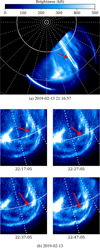 |
Fig. 5 Observation of the growth of a bridge-like arc in the northern aurora during the GO-15638 HST campaign. The bridge location is highlighted by the red arrow. The associated GIF images are available online. |
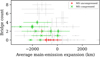 |
Fig. 6 Detected average expansion of the ME from Head et al. (2024) vs. the total detected bridge count for each northern HST-STIS series we considered. Negative expansions imply a contracted ME. The bridge-count error bars are determined as described in Appendix A.1. The green crosses denote the cases in which the magnetosphere was compressed, and red pluses show cases in which the magnetosphere was uncompressed. The grey points denote cases in which the compression state of the magnetosphere is unknown. |
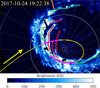 |
Fig. 7 Mapped Juno-footprint trajectory for PJ9-S overlaid on the UVS exemplar image (central spin time stamp in the top left corner). The yellow arrow indicates the direction of travel of Juno. The position of the Sun is marked by a solid orange line. The bridges are given in red and the ME in green. The Juno crossings of these arcs are given in magenta. |
3.4 Juno multi-instrument analysis
3.4.1 Case study of PJ9-S
By comparing the projected Juno ionospheric footprint against manually determined bridge positions in the base image of each hemisphere during each perijove, we determined approximate bridge-crossing time stamps and compared them against data and derived parameters from Juno. We mapped the Juno footprint in the ionosphere using field-line tracing of the JRM33 field model rather than flux-equivalence mapping because Juno is at a low altitude, which minimises the effect of the model inaccuracies in the polar region. This method can map the footprint within the entire polar region. An example of this analysis is given in Figures 7 and 8 for PJ9-S, in which Juno first passed over the ME (green) and then over three clear bridge-like structures in the dusk-side polar collar (red) at low altitude (~2 RJ), where the positions of these features were determined following Section 3.2. The crossing showed the expected FAC inversion (Al Saati et al. 2022; Mauk et al. 2020). Juno observed upward FACs (majority downward-travelling electrons) as it first passed through the ME and then downward FACs (majority upward-travelling electrons) as it continued into the polar collar. It is notable that the ME crossing was associated with uniquely upward FACs, rather than an inversion, indicating that the ME was a uniquely ZI feature during this crossing (Mauk et al. 2020). Unlike the ME crossing of PJ7-N described by Kurth et al. (2018), there was no significant Waves-E emission; instead, Juno started to observe significant plasma-wave emission after it entered into the polar collar, with high-frequency peaks occurring during bridge crossings that then abated after the third bridge. The calculated FACs remained downward for all three of these bridge crossings, although no particular peaks or signatures were observed that might be associated with the bridge. In particular, the lack of FAC inversion signatures during the bridge crossings suggests two things: firstly, that bridges are mechanically distinct from the ME, although they are morphologically related insofar as they can disrupt the morphology of the ME (Nichols et al. 2009a); and secondly, that vorticity in the dusk-side magnetosphere is likely not the source of the bridges, as was suggested previously (Fukazawa et al. 2006; Pardo-Cantos 2019), because this would be expected to give rise to noticeable FAC signatures (Delamere et al. 2013; Johnson et al. 2021). Additionally, there was no bridge-crossing signature in the derived Alfvénic Poynting flux, which indicates that the mechanisms that cause auroral moon footprints (Gershman et al. 2019) do not cause the bridges. During the first bridge crossing, Juno observed a clearly broadband bidirectional field-aligned electron distribution, although the upward electron energy flux was greater than the downward flux. This trend is stronger for the latter two crossings; while the electron distributions remain field-aligned and broadband, there is a clear preference for upward-travelling electrons. Only a small downward electron flux is required to produce the low auroral brightnesses associated with these bridge crossings, however, regardless of the upward electron flux. Peaks in the downward electron energy flux are present and coincide with the peaks in auroral brightness. It is notable that while plasma-wave emission can clearly be associated with these bridge crossings (and not with the ME crossing), the intensity of this emission does not appear to be correlated with the auroral brightness seen during the bridge crossings. The plasma-wave emission is also not constant during the crossings, although these peaks are not associated with any flaring behaviour in the bridges. This may indicate a more complex relation between these plasma waves and the generation of the aurora, if they are indeed related to the processes that give rise to bridges and are not merely coincident.
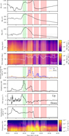 |
Fig. 8 Juno instrument data for PJ9-S. The ME crossing is first (dotted green) followed by three bridge crossings (dashed red). From top to bottom: Residual magnetic field components (FGM data; JRM33); JEDI electron energy; JEDI electron pitch-angle distribution (average given by the solid white line); JEDI field-aligned (0°-20°, 160°-180°) electron energy flux; UVS footprint brightness; calculated ionospheric FACs; calculated ionospheric Alfvénic Poynting flux (the step in the flux is related to a change in the operating range of the FGM instrument); and Waves-E LFR-Lo spectral density. |
3.4.2 Analysis of the first 30 perijoves
A similar analysis was performed for the first 30 perijoves, which are equivalent to 58 auroral crossings. Bridges are present in the dusk-side polar collar during 39 of these traversals, and Juno passes over at least one arc in 26 of these cases. Eleven of these traversals show aurorae without clear bridges. The remaining 8 cases have large gaps in the UVS coverage and were ignored. Bridges are present in a large fraction (at least 67%) of the first 30 perijoves. Of these perijoves, the presence or absence of bridges is mostly maintained between the northern and southern crossing; when Juno observed bridges in the northern aurora, it also typically saw bridges in the southern aurora ~2 hours later. This is in line with previous work, which suggested that bridges are stable over timescales of several hours (Nichols et al. 2009b), and it indicates that the processes that give rise to bridges are conjugate between hemispheres and thus likely occur on closed field lines. These bridges are noted to occur at similar local times and have comparable geometries, although more accurate magnetic field models are required to determine whether the bridges lie along the same field lines in the north and south. Only two perijoves (PJ4, PJ9) showed bridges that appeared or disappeared over the course of a perijove. During PJ4, a long faint bridge was visible in the northern aurora around 21 MLT, which had disappeared completely by the Juno pass over the southern aurora. During PJ9, the dusk-side polar collar was free of bridges (although the dusk-side ME was slightly non-continuous) during the northern pass; by the time of the southern Juno pass, three distinct bridges had developed. Combined with the result that bridges usually appear conjugate between the two hemispheres, this indicates that the process that causes bridges can occur over hour-long timescales. This is consistent with the result shown in Figure 5.
Bridge crossings at low altitudes were also generally associated with downward FACs (average for cases with altitudes below 3 RJ = −0.1±0.3 μA m−2) but without a particular signature (a peak during the crossing, for example), and broadband upward-dominated bidirectional electron distributions, as suggested by the results from PJ9-S. ME crossings, however, were more usually associated with upward FACs (average for cases with altitudes below 3 RJ = 0.2±0.7 μA m−2) or FAC inversions, although the large uncertainties make it challenging to differentiate the two features from their average currents alone.
Figure 9 shows an approximately linear relation (that passes through the origin) between the mean UV auroral brightnesses and downward electron energy fluxes seen by Juno during the bridge crossings. This is an indication that the downward electrons seen by Juno are indeed the source of the auroral emission associated with bridges. An electron energy flux of 1 mW m−2 is equivalent to an auroral brightness of 2.9 kR. This is a slightly lower brightness than previous estimates for the aurora (Mauk et al. 2017b; Nichols & Cowley 2022). This may be due to subtle implementation differences with previous work, or it might be a genuine difference from the canonical 1 mW m−2 = 10 kR in the case of bridges. This also assumes that the entire electron energy flux seen by Juno at the typical crossing altitude of ~2 RJ contributes toward the auroral brightness of the bridge. In the presence of a vertically extended acceleration region at or below the altitude of Juno (e.g. Sulaiman et al. 2022), some of the downward electron flux may be bidirectionally re-accelerated, reducing the downward flux that reaches the auroral layer.
In addition to the above relation between bridge auroral brightness and downward electron flux, the typical electron pitch-angle profiles seen during bridge and ME crossings (red in Figure 10) are also noteworthy; the crossings we used in this analysis are given in Figures B.5 to B.7 and Table C.1. These pitch-angle distributions are the average normalised profiles of bridge and ME crossings and not the average distribution to account for large differences in the total electron flux because the profile is the aspect of interest. Bridges are dominated by upward-travelling field-aligned electrons, but with a considerable downward component. The ME crossings were split into cases in which the ME crossing was immediately preceded or succeeded by a bridge (regardless of whether this was crossed by Juno) and cases without bridges in the vicinity of the ME crossing. The ME crossings with bridges (green) show electron distributions that are dominated by downward-going electrons. Cases without bridges (orange) have broadly symmetrical field-aligned electron populations, but there is a preference toward upward-travelling electrons. It is first worth noting that the presence or absence of bridges affects the properties of the ME auroral-electron population, not simply its morphology. Secondly, in the absence of a bridge, the ME electron population takes on a more bridge-like character, with a greater proportion of upward-travelling electrons. This indicates that the bridge is still present within the aurora, but is indistinguishable from the ME.
The three types of crossing also differ in the observed Waves-E LFR-Lo intensity, especially at higher frequencies (see Figure 11, where only the higher frequency portion (>1000 Hz) of the Waves-E LFR-Lo spectra was used to capture the spiking behaviour of the Waves-E signal seen in Figure 8). The high-frequency Waves-E intensity is noticeably higher than the polar-region background level (dotted grey line) for bridge crossings (red), which agrees with previous results (Sulaiman et al. 2022), and crossings of the ME when no bridges are present (orange). ME crossings with bridges (green) have noticeably lower high-frequency Waves-E LHR-Lo intensities comparable with the background, as seen in PJ9-S, and there is a clear distinction (in the 25th to 75th percentile range) from the other two crossing types. If increased Waves-E intensity can be associated with bridge crossings, as seen during PJ9-S and as indicated by Figure 11, then the ME appears to take on bridge-like traits in the absence of a discernable bridge, again indicating that the bridge emission is still present within the ME. As in PJ9-S, although this Waves-E intensity is increased during bridge crossings, it is not correlated with the auroral brightness, which may be due to a strong dependence on altitude or a genuine complex non-linearity in the associated acceleration process(es).
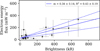 |
Fig. 9 Mean Juno-footprint UV auroral brightness vs. mean JEDI downward electron energy flux observed during low-altitude (<3 RJ) bridge crossings between PJ1 and PJ30. Uncertainties (grey) are estimated using the 50th and 100th-percentile values observed during crossings. The gradient and R2 value of the least-squares linear relation (solid blue line) is given in the legend. |
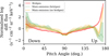 |
Fig. 10 Median-average JEDI electron flux vs. pitch angle profiles during low-altitude (<3 RJ) bridge crossings (solid red) and ME crossings, both with (dotted green) and without (dashed orange) local bridges, observed by Juno. The shaded regions denote the 25-to-75th percentile range. |
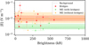 |
Fig. 11 Median high-frequency (>1000 Hz) WAVES-E LFR-Lo intensity vs. median UV Juno-footprint brightness during dusk-side (12<MLT<18) low-altitude (<3 RJ) bridge crossings (red cross) and ME crossings, both with (green plus) and without (orange dot) local bridges, observed by Juno. The error bars give the 25th and 75th percentile values during each crossing. The median WAVES-E intensity of each distribution is given by the dashed line, and the 25th to 75th percentile range is shown by the shaded areas. The background intensity is given by the dotted grey line. |
4 Discussion
Our results indicate that bridges show similarities with ZII aurora, as defined by Mauk et al. (2020). They preferentially coincide with the downward-FAC region poleward of the ME and show bidirectional electron distributions that are dominated by upward-travelling electrons, as in Figure 10. This tentative association between ZII aurora and bridges is notable because it would imply that the spacing between ZI (upward FAC) and ZII (downward FAC) aurora is variable, to such an extent that there is sometimes a considerable gap between the two (in this case, between the bridge and the rest of the ME). The presence or absence of bridges is also suggested to affect the properties of the ME. When bridges are present, the ME is dominated by downward-travelling electrons (see Figure 10), as expected of the ZI aurora. When bridges are instead absent, the ME electron distribution is typically more symmetric. The proposed interpretation is that bridges are ZII aurorae that have become spatially separated from the ZI aurora, such that in the absence of bridges, the ZII aurora is spatially indistinguishable from the ZI ME, leading to a more symmetric electron distribution during these ME crossings. This hypothesis is further supported by the stronger broadband plasma-wave signatures (considered to be a signature of ZII aurora; Sulaiman et al. 2022) seen during ME crossings in the absence of bridges (compared to those with bridges), as though the ZI and ZII aurorae are spatially adjacent (the typical configuration; Mauk et al. 2020). Even if future work weakens the association between bridges and ZII aurora, the fact that the presence of bridges affects not only the morphology, but also the electron populations of the ME is itself notable.
Pending sampling of the low-altitude dawn aurora by Juno, the distinction between ZI and ZII aurorae is expected to be a phenomenon that is present in the entire ME, although perhaps with some considerable dependence on the local time (Sulaiman et al. 2022), which may seem at odds with the idea that the bridge, a uniquely pre-dusk feature, can be identified as the ZII aurora. It was suggested that the process that gives rise to the separation between ZI and ZII in the case of bridges may occur more easily or to a greater extent in the pre-dusk magnetosphere. This is compatible with the analysis by Jenkins et al. (2024), in which the Alfvén radius was shown to be greater than 60 RJ only between 10 and 20 MLT, which limits the information that can be conveyed to the aurora from the distant magnetosphere beyond 60 RJ via Alfvén waves outside of these sectors; the bridge source process may similarly be hampered in the dawn and night sectors, which would explain the lack of observed bridges in these regions of the aurora. This interpretation is tentative and requires both modelling work and further data from Juno, and also a better understanding of the processes that give rise to bridges.
Our results also support the ZII auroral-generation scenario described by Elliott et al. (2018) and Sulaiman et al. (2022). In this scenario, electric potential structures above the ionosphere create upward electron beams that generate large-amplitude ESWs, as was demonstrated (Elliott et al. 2020). These ESWs provoke bidirectional broadband electron acceleration that leads to auroral emission. This scenario explains the presence of high-frequency Waves-E emission that is observed by Juno-Waves during bridge crossings (frequency-domain representations of large-amplitude ESWs; Sulaiman et al. 2022) and upward-dominated bidirectional broadband electrons observed by JEDI (the combination of upward electron beams and stochastic acceleration from ESWs). The association of enhanced Waves-E emission with bridge crossings indicated in this work, rather than with signatures in the FACs or Alfvénic Poynting flux, supports this scenario. ESWs, observed as enhanced Waves-E emission, are also associated with ME crossings in the absence of bridges, but not when bridges are present. This again supports the hypothesis that the bridge aurora remains present even when it is spatially indistinguishable from the ME, which is consistent with the association between bridges and ZII. While ESWs appear to be associated with bridge crossings, the expected acceleration processes are poorly understood and highly non-linear, and although Waves-E intensity peaks are systematically seen during bridge crossings, there is a lack of correlation between auroral brightness and Waves-E intensity, and the above scenario therefore remains speculative.
Our results also suggest that the solar wind exerts some influence on the morphology of the ZI and ZII aurorae. If magnetospheric compression can predominantly be attributed to the solar wind (rather than a variable plasma-outflow rate from Io), the agreement between bridge count and the compression state of the magnetosphere, shown in Figure 6, is consistent with the result of Nichols et al. (2017), who observed a bridge-like morphology in the dusk-side polar collar during a solar wind shock measured by Juno during its approach to Jupiter. The results regarding the onset times and lifetimes for bridges (that they can arise within a few hours and can last for longer than a Jupiter rotation) also fit this hypothesis, since hour-scale variations are compatible with simulations of the effect of solar wind shocks on the magnetosphere (Chané et al. 2017). Therefore, if ZI aurora can be spatially associated with upward Birkeland currents and ZII aurorae with the downward currents necessary to close the loop (Sulaiman et al. 2022), then the solar wind is suggested to affect the local ionospheric or magnetospheric conditions required for current-loop closure, thus affecting the morphology of the ZI and ZII aurorae. It may, to some extent, do this by modifying the magnetic topology within the middle Jupiter magnetosphere. Compression of the magnetosphere by the solar wind has already been shown to play a significant role in contracting the ME via modification of the current sheet and associated magnetic field contribution, rather than by modifying the ME magnetospheric source radius (Nichols et al. 2009a; Head et al. 2024). Our work may indicate that magnetospheric compression by the solar wind pushes the magnetic field lines inward, which would move ME features poleward and also increase the ionospheric separation between adjacent features in the magnetosphere. This scenario, though tentative, is consistent with bridges that grow from the ME rather than from the active region (Figure 5). Additionally, three ME crossings (PJ3-N, PJ14-N, PJ22-N) were identified by Al Saati et al. (2022) in which the ZII (downward FAC) region was located equatorward of the ZI region. These three cases all also showed expanded MEs (Head et al. 2024; supporting material), associated with an uncompressed magnetosphere, which may work in the opposite direction to pull the ZII aurorae equatorward of the ZI aurora, in contrast with previous predictions (Cowley et al. 2007). More work is required to investigate the exact mechanisms for the variation in morphology of the ZI and ZII aurorae, but, in all, this work suggests that the solar wind may exert an indirect but significant influence on the jovian aurorae.
5 Conclusions
We summarise our findings below:
Bridges are observed as dusk-side polar-collar arcs in the jovian UV aurora and are frequently seen in both hemispheres in HST-STIS and Juno-UVS images;
They are observed to appear and disappear on timescales of hours and have been seen to persist over a full Jupiter rotation. This agrees with previous conclusions made using limited data;
The appearance of bridges in the aurora is associated with compression of the magnetosphere;
Crossings of bridges by Juno are preferentially associated with downward FACs and broadband field-aligned electron distributions dominated by upward-travelling electrons, indicating that bridges are possibly ZII aurorae as defined by Mauk et al. (2020) that have become noticeably separated from the (ZI) ME. Where Juno passes at low (<3 RJ) altitude over the aurora, bridge crossings are also often associated with ESWs observed by Juno-Waves. This agrees with the scenario presented by Elliott et al. (2018) and Sulaiman et al. (2022), in which upward-travelling ESWs induce bidirectional broadband auroral electron acceleration;
The ME is typically associated with ESWs and largely symmetric bidirectional electron distributions when bridges are absent from the aurora and with predominantly downward electron populations without considerable ESWs when bridges are present. This suggests that the ME may exist as either an adjacent ZI+ZII aurora or as a uniquely ZI aurora when the ZII aurora has become spatially separated in the form of bridges;
Finally, the identification of the bridge as ZII aurora spatially separated from the ME, alongside the observed dependence of the appearance of bridges on the state of compression of the magnetosphere, implies that the solar wind can exert influence on the morphology of the jovian UV aurora.
Future numerical experiments are required to investigate the effect of various types of solar wind compression on the auroral morphology and to provide a theoretical explanation for the results described in this work.
Data availability
Juno data can be obtained from the NASA Planetary Data System (https://pds-atmospheres.nmsu.edu/data_and_services/atmospheres_data/JUNO/juno.html).
The movies associated to Fig. 5 are available at https://www.aanda.org
Movies
Movies associated to Fig. 5 Access Supplementary Material
Movies associated to Fig. 5 Access Supplementary Material
Movies associated to Fig. 5 Access Supplementary Material
Movies associated to Fig. 5 Access Supplementary Material
Movies associated to Fig. 5 Access Supplementary Material
Movies associated to Fig. 5 Access Supplementary Material
Movies associated to Fig. 5 Access Supplementary Material
Movies associated to Fig. 5 Access Supplementary Material
Movies associated to Fig. 5 Access Supplementary Material
Movies associated to Fig. 5 Access Supplementary Material
Movies associated to Fig. 5 Access Supplementary Material
Movies associated to Fig. 5 Access Supplementary Material
Movies associated to Fig. 5 Access Supplementary Material
Movies associated to Fig. 5 Access Supplementary Material
Movies associated to Fig. 5 Access Supplementary Material
Movies associated to Fig. 5 Access Supplementary Material
Movies associated to Fig. 5 Access Supplementary Material
Movies associated to Fig. 5 Access Supplementary Material
Movies associated to Fig. 5 Access Supplementary Material
Movies associated to Fig. 5 Access Supplementary Material
Acknowledgements
We are grateful to NASA and contributing institutions which have made the Juno mission possible. This work was funded by NASA’s New Frontiers Program for Juno via contract with the Southwest Research Institute. This publication benefits from the support of the French Community of Belgium in the context of the FRIA Doctoral Grant awarded to L.A. Head. B. Bonfond is a Research Associate of the Fonds de la Recherche Scientifique – FNRS. M.F. Vogt was supported by NASA grants 80NSSC17K0777 and 80NSSC20K0559. Data analysis was performed with the AMDA science analysis system provided by the Centre de Données de la Physique des Plasmas (CDPP) supported by CNRS, CNES, Observatoire de Paris and Université Paul Sabatier, Toulouse. A. Moirano is supported by the Fonds de la Recherche Scientifique – FNRS under Grant(s) No. T003524F.
Appendix A Description of methods
A.1 Bridge detection
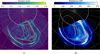 |
Fig. A.1 (a) Arc convolution of the auroral image shown in Figure 1. Red lines denote the mapped magnetopause (solid) and fixed-radius contours (dashed) described in the text. (b) Results of the bridge-detection algorithm after filtering. Red solid lines denote detected arcs identified as bridges. Dark-red dashed lines denote arcs identified as PAFs. The seed point of each arc is in magenta. Manually designated arcs are in green. White contours give the region of validity of the Vogt et al. (2011) JRM33 flux-equivalence mapping along closed field lines. |
Bridges are defined as arcs that connect the day-side active region to the main emission via the polar collar (though they may not span this gap fully). This implies that they traverse a significant radial distance in the magnetosphere, since the main emission is surmised to originate from a region between 20 and 40 RJ(Cowley & Bunce 2001), whereas the active region is firmly within the polar aurora and hence maps to more distant regions of the magnetosphere. Hence, a number of fixed-radius contours were projected to the ionosphere (75, 80, 85, 100, and 110 RJ), and the Joy et al. (2002) expanded magnetopause (stand-off distance 92 RJ; used as the outer boundary of validity in the Vogt et al. 2011 flux-equivalence model) which was observed to approximately coincide with the boundary between the polar collar and the day-side active region; see red contours in Figure A.1a. Here, the flux-equivalence mapping of Vogt et al. (2011) was used with the JRM33 magnetic field model (Connerney et al. 2022) since it is expected to be more reliable than field-line tracing in the polar aurora, though the choice of mapping method was a posteriori determined to not affect the conclusions of this work. The brightness along these mapped contours was determined and a broad uniform filter (0.3 MLT) applied. Peaks in the smoothed brightness were presumed to coincide with arcs that cross these contours. For each of these “seed” points, the arc was propagated in a stepwise fashion, by taking all pixels within a 11×11-pixel area around the seed pixel, calculating an effective path brightness for each pixel by averaging the brightness of all pixels between the seed and the target pixel (to ensure that the arc propagation algorithm does not jump over regions of dark pixels to arrive at a bright pixel), and adding the pixel with the greatest effective path brightness to the arc. This process is repeated for all seed pixels until one of the following conditions is met: the new best target pixel is already part of a different arc, at which point the two arcs can be merged; the target pixel maps to a magnetospheric radius that is more than 10 RJ from the radius of the previous pixel, which was determined to often coincide with a failure of the algorithm; the target pixel maps to a radius less than 50 RJ in the magnetosphere, at which point the algorithm is at risk of simply detecting the main emission; the target pixel has an arcness score below 0.2.
To ensure that the algorithm is indeed detecting bridges, manual designations were created (thick yellow arcs in Figure A.1b) for the northern-hemisphere image series in the STIS campaign GO-15638, which contains a total of 66 manually identified bridges over 42 image series. At this stage, the bridge-detection algorithm performs poorly; it does detect 90% of the manually identified bridges, but only 16% of the automatically detected bridges have a manual equivalent. Using the scikit-learn Python library, a random-forest classifier with a typical train-test split of 8:2 was trained on a number of detected-arc parameters (seed magnetosphere radial distance, seed magnetosphere local time, average arc brightness, average arc “arcness” value, total projected length of the arc in the magnetosphere). The optimal hyperparameters were determined using a randomised search with tree counts between 10 and 1000 and maximum tree depths between 3 and 50; a tree count of 912 and a maximum tree depth of 42 were found to be optimal, and resulted in a model test accuracy of 0.82 when applied to the test data. This classifier was then applied to the full set of automatically detected bridges as a filter, which increased the proportion of detected arcs with manual equivalents (of those cases where arcs had been identified manually) from 16% to 96%. An example of the filtered bridge arcs is given in Figure A.1b.
To estimate the uncertainty in the detected bridge count introduced by this method, a sensitivity analysis was performed by varying the cutoff arcness score between 0.1 and 0.3. The uncertainties in the detected bridge count shown in Figure 6 indicate the range of detected bridge counts introduced by varying this cutoff parameter.
A.2 Description of the field-aligned-current calculation
The method used to estimate the field-aligned-current (FAC) densities close to Jupiter uses data from the Juno FluxGate Magnetometer (FGM) instrument and is essentially an application of the method described in Al Saati et al. (2022). The interested reader is invited to consult the thorough description of this method provided in the supporting material of Al Saati et al. (2022). The method makes several key assumptions. Firstly, the ionosphere (auroral) layer is modelled as an infinitely thin shell; this is a reasonable approximation given the thickness of this layer compared to the scale of the jovian magnetosphere. Jupiter’s magnetic field is assumed to be dipolar, and hence the magnetic field lines radial close to the planet. The main emission is taken to run (locally) along a contour of constant magnetic latitude, and that magnetospheric-coupling parameters are (locally) constant along the field line and along the main emission, and only vary in the direction perpendicular to the contour of the main emission. Juno is assumed to be moving roughly perpendicularly to the background magnetic field, and perturbations in this magnetic field are assumed to be spatial, not temporal, since Juno cannot distinguish between the two (Sulaiman et al. 2023). Under these assumptions, Ampère’s law (in a vacuum and in the absence of a time-varying electric field)
![Mathematical equation: $\[\boldsymbol{J}=\frac{1}{\mu_0} \boldsymbol{\nabla} \times \boldsymbol{B},\]$](/articles/aa/full_html/2025/08/aa54759-25/aa54759-25-eq1.png) (A.1)
(A.1)
where J is the current density at Juno, μ0 is the permeability of free space, and B is the magnetic field at Juno, can be reduced to
![Mathematical equation: $\[J_{\|}=\frac{1}{\mu_0} \frac{\partial\left(\sin~ \theta \delta B_\phi\right)}{r ~\sin~ \theta \partial \theta},\]$](/articles/aa/full_html/2025/08/aa54759-25/aa54759-25-eq2.png) (A.2)
(A.2)
where δB denotes the magnetic field residuals obtained by subtracting a magnetic field model from the FGM magnetic field measurements (JRM09 in Al Saati et al. (2022), JRM33 in this work). By conservation of magnetic flux,
![Mathematical equation: $\[J_{\|, i o n o}=\frac{\left|B_{\text {iono }}\right|}{|B|} J_{\|},\]$](/articles/aa/full_html/2025/08/aa54759-25/aa54759-25-eq3.png) (A.3)
(A.3)
where Xiono refers to values determined for the ionosphere. Al Saati et al. (2022) also perform a Fourier filtering on their magnetic field residuals to remove superfluous frequencies that lay far from the frequency of their signal(s) of interest.
This work makes the same assumptions as Al Saati et al. (2022), barring the assumption of a dipolar magnetic field. Instead, the full magnetic field is taken into account when calculating ∇ × δB, and so the field-aligned currents are given by
![Mathematical equation: $\[J_{\|}=\left(\frac{1}{\mu_0} \boldsymbol{\nabla} \times \delta \boldsymbol{B}\right) \cdot \hat{B}_{J R M 33}.\]$](/articles/aa/full_html/2025/08/aa54759-25/aa54759-25-eq4.png) (A.4)
(A.4)
This does not greatly increase the computational effort required to estimate the field-aligned currents. Additionally, no Fourier filtering is performed on the magnetic field residuals since so particular signal frequency is targeted by this work. The implementation of this method was checked against the results presented in Al Saati et al. (2022) and found to agree exactly in all cases, and thus the method used in this work is considered to be verified against Al Saati et al. (2022), though the assumptions used in this work risk misrepresenting the true state of the auroral currents and should be investigated more thoroughly in a dedicated work.
Appendix B Supplementary figures
 |
Fig. B.1 Results of the bridge-detection algorithm after filtering for cases where the compression state of the magnetosphere is known (Yao et al. 2022; Louis et al. 2023). Red lines denote bridge-candidate arcs that correspond to manual designations, and grey the arcs that do not but are nevertheless accepted by the random-forest filter. Dark-red dashed lines are those arcs that are identified as PAFs rather than bridge candidates. The seed point of each arc is given in magenta. Manually designated arcs are given in yellow. White contours give the region of validity of the Vogt et al. (2011) JRM33 flux-equivalence mapping along closed field lines. HST exposure identifiers, central timestamps, and the compression state of the magnetosphere are given in the top left. |
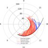 |
Fig. B.2 As Figure 3, but using field-line tracing of JRM33 (Connerney et al. 2022) and Con2020 (Connerney et al. 2020) to map the bridges from the aurora to the magnetosphere. |
 |
Fig. B.3 Detected bridge count vs total detected bridge magnetosphere-mapped length for the HST-STIS northern-hemisphere cases considered in section 3.3, expressed as a percentage of the total cases. There is an approximately linear relationship between bridge count and total bridge length. |
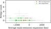 |
Fig. B.4 Detected average expansion of the ME from Head et al. (2024) vs the detected PAF count for each northern HST-STIS series considered in this work. Negative expansions imply a contracted ME. Green crosses denote those cases with a compressed magnetosphere, and red pluses those cases with an uncompressed magnetosphere (Yao et al. 2022); grey points denote cases where the compression state of the magnetosphere is unknown. |
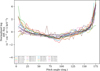 |
Fig. B.5 The normalised log JEDI electron differential flux pitch-angle profiles used to produce the average profile for bridge crossings in Figure 10 (red). The median-average profile is given as a black dashed line. The 25th- and 75th-percentile values are given as black dotted lines. |
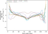 |
Fig. B.6 The normalised log JEDI electron differential flux pitch-angle profiles used to produce the average profile for main-emission crossings with nearby bridges in Figure 10 (green). The median-average profile is given as a black dashed line. The 25th- and 75th-percentile values are given as black dotted lines. |
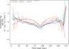 |
Fig. B.7 The normalised log JEDI electron differential flux pitch-angle profiles used to produce the average profile for main-emission crossings without nearby bridges in Figure 10 (orange). The median-average profile is given as a black dashed line. The 25th- and 75th-percentile values are given as black dotted lines. |
Appendix C Supplementary tables
Perijoves used in this work.
References
- Al Saati, S., Clément, N., Louis, C., et al. 2022, J. Geophys. Res.: Space Phys., 127, e2022JA030586 [NASA ADS] [CrossRef] [Google Scholar]
- Bagenal, F., & Delamere, P. A. 2011, J. Geophys. Res.: Space Phys., 116, A05209 [NASA ADS] [CrossRef] [Google Scholar]
- Bonfond, B., Grodent, D., Gérard, J.-C., et al. 2009, J. Geophys. Res., 114, A07224 [NASA ADS] [CrossRef] [Google Scholar]
- Bonfond, B., Gladstone, G. R., Grodent, D., et al. 2018, Geophys. Res. Lett., 45, 12108 [Google Scholar]
- Bonfond, B., Yao, Z. H., Gladstone, G. R., et al. 2021, AGU Adv., 2, e2020AV000275 [CrossRef] [Google Scholar]
- Chané, E., Saur, J., Keppens, R., & Poedts, S. 2017, J. Geophys. Res.: Space Phys., 122, 1960 [CrossRef] [Google Scholar]
- Connerney, J. E. P., Benn, M., Bjarno, J. B., et al. 2017, Space Sci. Rev., 213, 39 [Google Scholar]
- Connerney, J. E. P., Timmins, S., Herceg, M., & Joergensen, J. L. 2020, J. Geophys. Res.: Space Phys., 125, e2020JA028138 [CrossRef] [Google Scholar]
- Connerney, J. E. P., Timmins, S., Oliversen, R. J., et al. 2022, J. Geophys. Res.: Planets, 127, e2021JE007055 [NASA ADS] [CrossRef] [Google Scholar]
- Cowley, S. W. H., & Bunce, E. J. 2001, Planet. Space Sci., 49, 1067 [NASA ADS] [CrossRef] [Google Scholar]
- Cowley, S. W. H., Bunce, E. J., Stallard, T. S., & Miller, S. 2003, Geophys. Res. Lett., 30, 1220 [Google Scholar]
- Cowley, S. W. H., Nichols, J. D., & Andrews, D. J. 2007, Ann. Geophys., 25, 1433 [NASA ADS] [CrossRef] [Google Scholar]
- Delamere, P. A., Wilson, R. J., Eriksson, S., & Bagenal, F. 2013, J. Geophys. Res.: Space Phys., 118, 393 [CrossRef] [Google Scholar]
- Elliott, S. S., Gurnett, D. A., Kurth, W. S., et al. 2018, J. Geophys. Res.: Space Phys., 123, 7523 [NASA ADS] [CrossRef] [Google Scholar]
- Elliott, S. S., Gurnett, D. A., Yoon, P. H., et al. 2020, J. Geophys. Res.: Space Phys., 125, e2020JA027868 [Google Scholar]
- Fukazawa, K., Ogino, T., & Walker, R. J. 2006, J. Geophys. Res.: Space Phys., 111, A10207 [Google Scholar]
- Gershman, D. J., Connerney, J. E. P., Kotsiaros, S., et al. 2019, Geophys. Res. Lett., 46, 7157 [Google Scholar]
- Gladstone, G. R., Persyn, S. C., Eterno, J. S., et al. 2017, Space Sci. Rev., 213, 447 [Google Scholar]
- Greathouse, T., Gladstone, R., Versteeg, M., et al. 2021, J. Geophys. Res.: Planets, 126, e2021JE006954 [CrossRef] [Google Scholar]
- Grodent, D. 2015, Space Sci. Rev., 187, 23 [CrossRef] [Google Scholar]
- Grodent, D., Clarke, J. T., Kim, J., Waite, J. H., & Cowley, S. W. H. 2003, J. Geophys. Res., 108, 1389 [Google Scholar]
- Groulard, A., Bonfond, B., Grodent, D., et al. 2024, Icarus, 413, 116005 [NASA ADS] [CrossRef] [Google Scholar]
- Gustin, J., Bonfond, B., Grodent, D., & Gérard, J.-C. 2012, J. Geophys. Res.: Space Phys., 117, A07316 [NASA ADS] [CrossRef] [Google Scholar]
- Génot, V., Budnik, E., Jacquey, C., et al. 2021, Planet. Space Sci., 201, 105214 [CrossRef] [Google Scholar]
- Head, L. A., Grodent, D., Bonfond, B., et al. 2024, A&A, 688, A205 [NASA ADS] [CrossRef] [EDP Sciences] [Google Scholar]
- James, M. K., Provan, G., Kamran, A., et al. 2022, https://doi.org/10.5281/zenodo.10602418 [Google Scholar]
- Jeandet, A., & Schulz, A. 2024, https://doi.org/10.5281/zenodo.12656220 [Google Scholar]
- Jenkins, A., Ray, L. C., Fell, T., Badman, S. V., & Lorch, C. T. S. 2024, J. Geophys. Res.: Planets, 129, e2024JE008414 [Google Scholar]
- Johnson, J. R., Wing, S., Delamere, P., Petrinec, S., & Kavosi, S. 2021, J. Geophys. Res.: Space Phys., 126, e2020JA028583 [Google Scholar]
- Joy, S. P., Kivelson, M. G., Walker, R. J., et al. 2002, J. Geophys. Res.: Space Phys., 107, SMP 17 [Google Scholar]
- Katsanis, R. M., & McGrath, M. A. 1998, The Calstis IRAF Calibration Tools for STIS Data, Tech. rep. [Google Scholar]
- Kurth, W. S., Hospodarsky, G. B., Kirchner, D. L., et al. 2017, Space Sci. Rev., 213, 347 [Google Scholar]
- Kurth, W. S., Mauk, B. H., Elliott, S. S., et al. 2018, Geophys. Res. Lett., 45, 9372 [Google Scholar]
- Louis, C. K., Jackman, C. M., Hospodarsky, G., et al. 2023, J. Geophys. Res.: Space Phys., 128, e2022JA031155 [Google Scholar]
- Mauk, B. H., Haggerty, D. K., Jaskulek, S. E., et al. 2017a, Space Sci. Rev., 213, 289 [Google Scholar]
- Mauk, B. H., Haggerty, D. K., Paranicas, C., et al. 2017b, Geophys. Res. Lett., 44, 4410 [CrossRef] [Google Scholar]
- Mauk, B. H., Clark, G., Gladstone, G. R., et al. 2020, J. Geophys. Res.: Space Phys., 125, e2019JA027699 [CrossRef] [Google Scholar]
- Nichols, J. D., & Cowley, S. W. H. 2022, J. Geophys. Res.: Space Phys., 127, e2021JA030040 [NASA ADS] [CrossRef] [Google Scholar]
- Nichols, J. D., Bunce, E. J., Clarke, J. T., et al. 2007, J. Geophys. Res.: Space Phys., 112, A02203 [Google Scholar]
- Nichols, J. D., Clarke, J. T., Gérard, J. C., & Grodent, D. 2009a, Geophys. Res. Lett., 36, L08101 [Google Scholar]
- Nichols, J. D., Clarke, J. T., Gérard, J. C., Grodent, D., & Hansen, K. C. 2009b, J. Geophys. Res.: Space Phys., 114, A06210 [NASA ADS] [Google Scholar]
- Nichols, J. D., Badman, S. V., Bagenal, F., et al. 2017, Geophys. Res. Lett., 44, 7643 [NASA ADS] [CrossRef] [Google Scholar]
- Palmaerts, B. et al. 2023, Icarus, 115815 [Google Scholar]
- Pardo-Cantos, I. 2019, Master’s thesis, Université de Liège, Belgium [Google Scholar]
- Sulaiman, A. H., Mauk, B. H., Szalay, J. R., et al. 2022, J. Geophys. Res.: Space Phys., 127, e2022JA030334 [CrossRef] [Google Scholar]
- Sulaiman, A. H., Szalay, J. R., Clark, G., et al. 2023, Geophys. Res. Lett., 50, e2023GL103456 [Google Scholar]
- Vogt, M. F., Kivelson, M. G., Khurana, K. K., et al. 2011, J. Geophys. Res.: Space Phys., 116, A03220 [Google Scholar]
- Wilson, R. J., Vogt, M. F., Provan, G., et al. 2023, Space Sci. Rev., 219, 15 [NASA ADS] [CrossRef] [Google Scholar]
- Yao, Z. H., Bonfond, B., Grodent, D., et al. 2022, J. Geophys. Res.: Space Phys., 127, e2021JA029894 [NASA ADS] [CrossRef] [Google Scholar]
All Tables
All Figures
|
Fig. 1 300-second image of the northern jovian UV aurora captured by HST during the GO-15638 campaign (exposure ID: odxc01okq). A 15° × 15° grid in System-III longitude and planetocentric latitude is included; the System-III longitude of certain meridians is given in white, and certain planetocentric latitudes are shown in magenta. The average subsolar longitude during this exposure (170°) is denoted by the solid yellow line, and the positions of the dawn and dusk hemispheres are included for guidance. The approximate location of the polar collar is enclosed by dashed red lines and the location of the noon active region by a dashed green ellipse. The bridges are highlighted with yellow arrows. |
| In the text | |
|
Fig. 2 Results of the bridge-detection algorithm after filtering. The solid red lines denote detected arcs that were identified as bridges. The dashed dark red lines denote arcs that were identified as PAFs. The seed point of each arc is shown in magenta. Manually designated arcs are plotted in green. The white contours delineate the validity region of the Vogt et al. (2011) JRM33 flux-equivalence mapping along closed field lines. |
| In the text | |
|
Fig. 3 Automatically detected bridge and PAF-like arcs (in pale red and blue) in all northern-hemisphere HST-STIS observations we considered, mapped via flux-equivalence mapping to the magnetospheric equator (radius and local time). The radii are given in RJ. A set of average bridge and PAF contours is given in dark red and blue; their starting locations on the Joy et al. (2002) expanded magnetopause (solar wind ram pressure = 0.039 nPa; stand-off distance 92 RJ) are given in black. |
| In the text | |
|
Fig. 4 Observation of a persistent bridge-like arc over a full Jupiter rotation in the southern aurora during the GO-14634 HST campaign. The bridge location is highlighted by the red arrow. This bridge is also present in the intervening HST and UVS (PJ6) observations. |
| In the text | |
|
Fig. 5 Observation of the growth of a bridge-like arc in the northern aurora during the GO-15638 HST campaign. The bridge location is highlighted by the red arrow. The associated GIF images are available online. |
| In the text | |
|
Fig. 6 Detected average expansion of the ME from Head et al. (2024) vs. the total detected bridge count for each northern HST-STIS series we considered. Negative expansions imply a contracted ME. The bridge-count error bars are determined as described in Appendix A.1. The green crosses denote the cases in which the magnetosphere was compressed, and red pluses show cases in which the magnetosphere was uncompressed. The grey points denote cases in which the compression state of the magnetosphere is unknown. |
| In the text | |
|
Fig. 7 Mapped Juno-footprint trajectory for PJ9-S overlaid on the UVS exemplar image (central spin time stamp in the top left corner). The yellow arrow indicates the direction of travel of Juno. The position of the Sun is marked by a solid orange line. The bridges are given in red and the ME in green. The Juno crossings of these arcs are given in magenta. |
| In the text | |
|
Fig. 8 Juno instrument data for PJ9-S. The ME crossing is first (dotted green) followed by three bridge crossings (dashed red). From top to bottom: Residual magnetic field components (FGM data; JRM33); JEDI electron energy; JEDI electron pitch-angle distribution (average given by the solid white line); JEDI field-aligned (0°-20°, 160°-180°) electron energy flux; UVS footprint brightness; calculated ionospheric FACs; calculated ionospheric Alfvénic Poynting flux (the step in the flux is related to a change in the operating range of the FGM instrument); and Waves-E LFR-Lo spectral density. |
| In the text | |
|
Fig. 9 Mean Juno-footprint UV auroral brightness vs. mean JEDI downward electron energy flux observed during low-altitude (<3 RJ) bridge crossings between PJ1 and PJ30. Uncertainties (grey) are estimated using the 50th and 100th-percentile values observed during crossings. The gradient and R2 value of the least-squares linear relation (solid blue line) is given in the legend. |
| In the text | |
|
Fig. 10 Median-average JEDI electron flux vs. pitch angle profiles during low-altitude (<3 RJ) bridge crossings (solid red) and ME crossings, both with (dotted green) and without (dashed orange) local bridges, observed by Juno. The shaded regions denote the 25-to-75th percentile range. |
| In the text | |
|
Fig. 11 Median high-frequency (>1000 Hz) WAVES-E LFR-Lo intensity vs. median UV Juno-footprint brightness during dusk-side (12<MLT<18) low-altitude (<3 RJ) bridge crossings (red cross) and ME crossings, both with (green plus) and without (orange dot) local bridges, observed by Juno. The error bars give the 25th and 75th percentile values during each crossing. The median WAVES-E intensity of each distribution is given by the dashed line, and the 25th to 75th percentile range is shown by the shaded areas. The background intensity is given by the dotted grey line. |
| In the text | |
|
Fig. A.1 (a) Arc convolution of the auroral image shown in Figure 1. Red lines denote the mapped magnetopause (solid) and fixed-radius contours (dashed) described in the text. (b) Results of the bridge-detection algorithm after filtering. Red solid lines denote detected arcs identified as bridges. Dark-red dashed lines denote arcs identified as PAFs. The seed point of each arc is in magenta. Manually designated arcs are in green. White contours give the region of validity of the Vogt et al. (2011) JRM33 flux-equivalence mapping along closed field lines. |
| In the text | |
|
Fig. B.1 Results of the bridge-detection algorithm after filtering for cases where the compression state of the magnetosphere is known (Yao et al. 2022; Louis et al. 2023). Red lines denote bridge-candidate arcs that correspond to manual designations, and grey the arcs that do not but are nevertheless accepted by the random-forest filter. Dark-red dashed lines are those arcs that are identified as PAFs rather than bridge candidates. The seed point of each arc is given in magenta. Manually designated arcs are given in yellow. White contours give the region of validity of the Vogt et al. (2011) JRM33 flux-equivalence mapping along closed field lines. HST exposure identifiers, central timestamps, and the compression state of the magnetosphere are given in the top left. |
| In the text | |
|
Fig. B.2 As Figure 3, but using field-line tracing of JRM33 (Connerney et al. 2022) and Con2020 (Connerney et al. 2020) to map the bridges from the aurora to the magnetosphere. |
| In the text | |
|
Fig. B.3 Detected bridge count vs total detected bridge magnetosphere-mapped length for the HST-STIS northern-hemisphere cases considered in section 3.3, expressed as a percentage of the total cases. There is an approximately linear relationship between bridge count and total bridge length. |
| In the text | |
|
Fig. B.4 Detected average expansion of the ME from Head et al. (2024) vs the detected PAF count for each northern HST-STIS series considered in this work. Negative expansions imply a contracted ME. Green crosses denote those cases with a compressed magnetosphere, and red pluses those cases with an uncompressed magnetosphere (Yao et al. 2022); grey points denote cases where the compression state of the magnetosphere is unknown. |
| In the text | |
|
Fig. B.5 The normalised log JEDI electron differential flux pitch-angle profiles used to produce the average profile for bridge crossings in Figure 10 (red). The median-average profile is given as a black dashed line. The 25th- and 75th-percentile values are given as black dotted lines. |
| In the text | |
|
Fig. B.6 The normalised log JEDI electron differential flux pitch-angle profiles used to produce the average profile for main-emission crossings with nearby bridges in Figure 10 (green). The median-average profile is given as a black dashed line. The 25th- and 75th-percentile values are given as black dotted lines. |
| In the text | |
|
Fig. B.7 The normalised log JEDI electron differential flux pitch-angle profiles used to produce the average profile for main-emission crossings without nearby bridges in Figure 10 (orange). The median-average profile is given as a black dashed line. The 25th- and 75th-percentile values are given as black dotted lines. |
| In the text | |
Current usage metrics show cumulative count of Article Views (full-text article views including HTML views, PDF and ePub downloads, according to the available data) and Abstracts Views on Vision4Press platform.
Data correspond to usage on the plateform after 2015. The current usage metrics is available 48-96 hours after online publication and is updated daily on week days.
Initial download of the metrics may take a while.