| Issue |
A&A
Volume 700, August 2025
|
|
|---|---|---|
| Article Number | A157 | |
| Number of page(s) | 16 | |
| Section | Astronomical instrumentation | |
| DOI | https://doi.org/10.1051/0004-6361/202555005 | |
| Published online | 14 August 2025 | |
Revisiting the differential optical transfer function wavefront sensing technique for high-contrast imaging
Université Côte d’Azur, Observatoire de la Côte d’Azur, CNRS,
Laboratoire Lagrange,
France
★ Corresponding author: This email address is being protected from spambots. You need JavaScript enabled to view it.
Received:
2
April
2025
Accepted:
7
July
2025
Abstract
Context. Wavefront sensors (WFSs) are widely used in optical measurements. Initially developed more than 40 years ago for adaptive optics (AO) systems in astronomy, they have become essential components in various stages of high dynamic range imaging systems.
Aims. The differential optical transfer function (dOTF) is a wavefront sensing technique that estimates the complex field of the pupil using differential intensities in the image plane. dOTF has a wide range of applications in astronomy, from optical shop testing to cophasing of segmented optics. This study aims to expand the application of dOTF from classical to high-contrast imaging.
Methods. Building on prior analyses in the literature, where the dOTF phase estimator was derived under the small-phase approximation and applied in classical imaging mode, we reformulated the phase estimator and extended it to include amplitude aberrations. This reformulation enabled the reconstruction of the complete electric field, allowing us to assess its applicability to dark hole digging, and to measure and correct non-common path aberrations (NCPAs) and cophasing misalignments, in coronagraphic imaging mode. Our findings are validated through comprehensive simulations, statistical analysis, and supported by preliminary experimental data.
Results. With a single-actuator probe, the dOTF demonstrates effective joint phase and amplitude wavefront sensing in coronagraphic imaging mode, without prior knowledge of the coronagraph type, a capability not previously documented. Beyond its capability to correct for NCPAs and cophasing misalignment, dOTF provides a simplified alternative to pair-wise probing (PWP) wavefront sensing.
Conclusions. The dOTF enables straightforward complex field measurement, with the deformable mirror (DM) actively participating in the process. By reducing imaging workload, it offers a promising alternative to other coronagraphic wavefront sensors. Its potential for high-contrast imaging has implications for current telescopes, upcoming missions like the Nancy Grace Roman Space Telescope, future large observatories, and laboratory conditions during instrument AIT phases.
Key words: instrumentation: adaptive optics / instrumentation: high angular resolution / methods: numerical / techniques: high angular resolution / telescopes
© The Authors 2025
 Open Access article, published by EDP Sciences, under the terms of the Creative Commons Attribution License (https://creativecommons.org/licenses/by/4.0), which permits unrestricted use, distribution, and reproduction in any medium, provided the original work is properly cited.
This article is published in open access under the Subscribe to Open model. This email address is being protected from spambots. You need JavaScript enabled to view it. to support open access publication.
1 Introduction
One of the main obstacles that prevent coronagraphs from fully blocking starlight is the presence of aberrations that cause starlight to leak into the coronagraphic image, creating speckle patterns with varying temporal characteristics (e.g., Racine et al. 1999; Guyon 2004; Hinkley et al. 2007; Martinez et al. 2013; Milli et al. 2016). These speckles can mimic planets in the final image, making detection challenging. To address this, deformable mirrors (DMs) correct wavefront errors before the light reaches the coronagraphic mask. This requires a carefully optimized set of technologies to correct dynamic, quasi-static, and static aberrations.
At both the observatory and the scientific instrument levels (adaptive optics, cophasing optics, extreme adaptive optics, fine cophasing optics, optical stability monitoring through wavefront sensing and control, image sharpening, coronagraphy, wavefront shaping, etc.), numerous wavefront sensors have been developed to tackle this challenge. In this context, most high-dynamic-range imaging instruments currently in development include coronagraphic wavefront sensing. To reach the extremely high contrasts required for imaging Earth-like planets, quasi-static speckles must be sensed and compensated for, while real-time monitoring, fine-tuning phasing errors, and temporal stability control during on-sky observation will be crucial for the next generation of large-segmented telescopes.
Wavefront sensing using a control loop around the DMs and the final science image allows for accurate wavefront estimation and control to compensate for non-common path aberrations (NCPAs) and ultimately to create a dark hole. This process, known as dark hole digging, involves actively conjugating the electric field in a closed-loop fashion. In recent years, several innovative methods of dark hole digging have emerged, and are being tested on the ground (e.g., Potier et al. 2020b, 2022; Galicher et al. 2024) and are envisioned on space missions (e.g., Bailey et al. 2023; Vaughan et al. 2023).
In this context, active minimization of the stellar speckle intensity in a coronagraphic image involves a focal plane wavefront sensor (FPWFS) that measures the wavefront from the science image and a wavefront controller (WFC) that drives the DMs to shape the wavefront. FPWFS can be based on spatial modulations (e.g., Baudoz et al. 2006; Galicher et al. 2008, 2010; Mazoyer et al. 2013; Martinache 2013; Mazoyer 2014; Delorme et al. 2016) of speckle intensity, temporal modulations (e.g., Bordé & Traub 2006; Give’on et al. 2007a, 2011; Paul et al. 2013b,a), or both (Martinez 2019). For WFC, energy minimization (Malbet et al. 1995; Bordé & Traub 2006) or electric field conjugation (EFC, Give’on et al. 2007b) algorithms are widely used, incorporating various regularization terms (Pueyo et al. 2009; Mazoyer et al. 2018; Herscovici-Schiller et al. 2018) to adapt to different scenarios. The most popular combination of WFS and WFC is pairwise probing (PWP) and EFC, although both are model-dependent and thus require accurate optical models of complex instruments. The recently proposed implicit EFC (iEFC, Haffert et al. 2023; Ahn et al. 2023) is a model-free version of conventional PWP/EFC derived in the context of PWP.
The dOTF wavefront sensor (Codona 2012, 2013; Codona & Doble 2015) is a phase-retrieval method that estimates the complex field by comparing two non coronagraphic images captured in the system’s focal plane, one of which includes a slight pupil modification. These modifications can affect the phase, amplitude, or both within the pupil. In high-contrast imaging setups that use DMs, implementing pupil modifications through DM actuator adjustments is straightforward, making it easy to integrate dOTF into existing optical systems without major hardware changes (e.g., Soummer et al. 2024; Dharmadhikari et al. 2024).
The dOTF method offers several key advantages: (i) it is model-independent, meaning it does not rely on a predefined model of the optical system, which can be difficult to obtain; (ii) it compares two differential images of the optical transfer function in the system’s focal plane, which reduces computational load and minimizing error propagation, and reduces the risk of NCPAs and vignetting effects; (iii) because both wavefront sensing and correction can be accomplished using a single deformable mirror, dOTF is highly practical in environments where complexity tends to increase.
However, a significant challenge in the broader application of dOTF for high-contrast imaging is adapting it for use in coronagraphic systems. To our knowledge, this capability has not yet been explored in the existing literature. Successfully extending dOTF for coronagraphic observing runs could enable its use for various objectives (NCPAs correction, cophasing monitoring, and dark-hole generation), offering a new, simple, and model-free wavefront sensor for these applications.
The paper is structured as follows: in Sect. 2, we review the dOTF theory and express phase and amplitude aberration estimators to estimate the electric field from coronagraphic images. Section 3 introduces our testing environments and Section 4 presents a series of simulations designed to demonstrate the performance of coronagraphic dOTF, including NCPAs, precise cophasing correction, and dark hole generation, all conducted within a comprehensive end-to-end emulator that mimics the SPEED (Segmented Pupil Experiment for Exoplanet Detection, Martinez et al. 2023a) test-bed. The SPEED project is a key experimental facility developed to investigate high-contrast imaging techniques with a segmented telescope, aiming to achieve extremely small angular separations in preparation for the next generation of ground- and space-based observatories. In Sect. 5, we present preliminary experimental results from the SPEED facility. Finally, in Sect. 6, we conclude.
2 Theory
In this section, after presenting our formalism and light propagation model, we provide a review of dOTF theory. Finally, we derive and express phase and amplitude aberration estimators used in coronagraphic observations.
2.1 Formalism and conventions
The star electric field measured on the science detector, in classical imaging (in the absence of a coronagraph), is noted ψs, and by 𝒞 we express the linear operator that transforms the complex electric field from the pupil to the science detector. By A we define the electric field in the pupil plane free from aberrations. The pupil phase, denoted ϕ, is composed of α and β that are the log-amplitude and phase aberrations, respectively. For the sake of simplicity, pupil and image variables are omitted. The symbol λ is the wavelength of observation. Under these assumptions, the complex pupil electric field is expressed as
![Mathematical equation: $\[\Psi_{s}=A \times e^{(\alpha+i \beta)} \times e^{(i \phi)},\]$](/articles/aa/full_html/2025/08/aa55005-25/aa55005-25-eq1.png) (1)
(1)
and the star electric field at the detector plane, ψs can be expressed as
![Mathematical equation: $\[\psi_{s}=C\left[A \times e^{(\alpha+i \beta)} \times e^{(i \phi)}\right],\]$](/articles/aa/full_html/2025/08/aa55005-25/aa55005-25-eq2.png) (2)
(2)
where ϕ is the phase introduced by a DM that is assumed in a pupil plane. We define ϕ as the potential composition of two different contributions such that ϕ = ϕcorr + ϕprobe, where ϕcorr corresponds to the phase introduced by the DM to alter the wavefront error, and ϕprobe the phase probe(s) used to measure the electric field. Assuming scenarios where aberrations and deformations on the DM (correction and probes) are small, and using the Taylor expansion of Eq. (2), ψs can be further developed as
![Mathematical equation: $\[\psi_{s}=C\left[A \times e^{(\alpha+i \beta)}\right]+i C[A \times \phi],\]$](/articles/aa/full_html/2025/08/aa55005-25/aa55005-25-eq3.png) (3)
(3)
where ψs finally can be expressed as
![Mathematical equation: $\[\psi_{s}=\psi_{s_{0}}+\psi_{D M}.\]$](/articles/aa/full_html/2025/08/aa55005-25/aa55005-25-eq4.png) (4)
(4)
Equation (4) comprises two terms: the first term corresponds to stellar speckles caused by aberrations, including contributions from α and β, while the second term represents speckles that can be induced by the DM either to compensate for the first term or to measure it. Since the detector provides access only to the squared modulus of ψs0, retrieving the field ψs0 requires the use of a wavefront sensor.
Interpreting or extracting the complex field from a pupil or PSF image is inherently challenging, as aberration signs are often ambiguous or lost. To overcome this, numerous methods have been developed, making image-based wavefront sensing a highly active area of research. These methods estimate the complex field by modifying the imaging system (e.g., Baudoz et al. 2006; Martinache 2013; Martinez 2019) or using pairs or sets of images (e.g., Bordé & Traub 2006; Give’on et al. 2007a, 2011), each obtained under specific, controlled modifications to the system (e.g., Paul et al. 2013a). Examples include shifting the focus or introducing known phase or amplitude aberrations to introduce data diversity. A solution is obtained by combining these controlled variations with prior information, such as an accurate optical system model or a theoretical PSF expression. Many of theses wavefront sensors have been adapted for coronagraphic systems by incorporating the effects of the coronagraph into the system model.
2.2 Classical imaging dOTF
The theory of dOTF is well-documented in the literature (Codona 2012, 2013; Codona & Doble 2015); here, we focus solely on its most essential aspects. The dOTF uses two point spread functions (PSFs): one corresponding to the nominal pupil condition and the other to a modified pupil condition. The pupil modification can be easily achieved by introducing a phase probe, such as an actuator motion. The PSFs for both conditions are then inverse Fourier transformed to derive the two corresponding OTFs. The OTF, denoted 𝒪, can be expressed as the auto-correlation of the pupil field Ψs0. These two OTFs are then subtracted to obtain the dOTF. The schematic representation of the dOTF estimate is presented in Fig. 1.
Assuming that 𝒪1 represents the OTF with an actuator poke and 𝒪0 denotes the unmodified OTF, the dOTF expression, denoted δ𝒪, can be written as:
![Mathematical equation: $\[\delta \mathcal{O}=\mathcal{O}_{1}-\mathcal{O}_{0},\]$](/articles/aa/full_html/2025/08/aa55005-25/aa55005-25-eq5.png) (5)
(5)
where
![Mathematical equation: $\[\mathcal{O}_{0}=\Psi_{s_{0}} \otimes \Psi_{s_{0}}^{*},\]$](/articles/aa/full_html/2025/08/aa55005-25/aa55005-25-eq6.png) (6)
(6)
where the symbol * and ⊗ represents the complex conjugate and the convolution product, respectively, and where
![Mathematical equation: $\[\mathcal{O}_{1}=\left(\Psi_{s_{0}}+\Psi_{D M_{probe}}\right) \otimes\left(\Psi_{s_{0}}+\Psi_{D M_{probe}}\right)^{*}.\]$](/articles/aa/full_html/2025/08/aa55005-25/aa55005-25-eq7.png) (7)
(7)
Equation (5) can be further expressed as
![Mathematical equation: $\[\delta \mathcal{O}=\Psi_{s_{0}} \otimes \Psi_{D M_{probe}}^{*}+\Psi_{D M_{probe}} \otimes \Psi_{s_{0}}^{*}+\Psi_{D M_{probe}} \otimes \Psi_{D M_{probe}}^{*}.\]$](/articles/aa/full_html/2025/08/aa55005-25/aa55005-25-eq8.png) (8)
(8)
As shown in Eq. (8) and illustrated in Fig. 1, the dOTF comprises three terms,
![Mathematical equation: $\[\delta \mathcal{O}=\delta \mathcal{O}_{+}+\delta \mathcal{O}_{-}+\delta \mathcal{O}_{\delta \delta},\]$](/articles/aa/full_html/2025/08/aa55005-25/aa55005-25-eq9.png) (9)
(9)
each being a correlation between the unmodified pupil field (Ψs0) and the pupil modification (ΨDMprobe). The first term (δ𝒪+) corresponds to the field in the pupil region convolved by the pupil modification introduced by the DM. The second term (δ𝒪−) is the conjugate of the first term, reflected about the point where the pupil modification was introduced, providing redundant information (see red and blue circles in Fig. 1). The last term (δ𝒪δδ) is the quadratic term where the first two terms overlap at the location of the pupil modification, related to the auto-convolution of the pupil modification. The overlap region between the first and second terms depends on the placement of the DM probe on the pupil.
The complex pupil electric field, including any aberrations and transmission effects introduced during propagation through the optical system, can be estimated to the spatial scale of the probe, by excluding the small overlap region. The pupil phase and amplitude can be retrieved from one of the two redundant pupil fields (δ𝒪+for instance)
![Mathematical equation: $\[\phi_{0}=arg \left\{\delta \mathcal{O}_{+}\right\},\]$](/articles/aa/full_html/2025/08/aa55005-25/aa55005-25-eq10.png) (10)
(10)
and the pupil amplitude from
![Mathematical equation: $\[\gamma=\left|\delta \mathcal{O}_{+}\right|.\]$](/articles/aa/full_html/2025/08/aa55005-25/aa55005-25-eq11.png) (11)
(11)
We note that, following our notations, γ = eα.
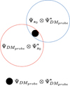 |
Fig. 1 Conceptual drawing of the dOTF contents. |
2.3 dOTF in the small aberrations regime
By removing the redundant information from Eq. (8) (second term) and by neglecting the third term (cross term, see Appendix A for a specific discussion on the cross terms), we can restrict the analysis to the first term, δ𝒪+, from Eq. (8), where
![Mathematical equation: $\[\delta O_{+}=\Psi_{s_{0}} \otimes \Psi_{D M_{probe}}^{*}.\]$](/articles/aa/full_html/2025/08/aa55005-25/aa55005-25-eq12.png) (12)
(12)
Assuming that the pupil modification is purely a phase term that induces only minor phase changes, we can express ![Mathematical equation: $\[\Psi_{D M_{probe}}^{*} \approx i \phi_{probe}\]$](/articles/aa/full_html/2025/08/aa55005-25/aa55005-25-eq13.png) . Here, ϕprobe can be approximated by a Gaussian function or a near-Dirac function (δ) if we use an actuator poke as a probe.
. Here, ϕprobe can be approximated by a Gaussian function or a near-Dirac function (δ) if we use an actuator poke as a probe.
Under the small phase approximation, linearizing the electric field, by combining Eq. (1) and Eq. (12) and by dropping the second-order terms (iαβ), Eq. (12) can be expressed as
![Mathematical equation: $\[\Psi_{s_{0}} \otimes \Psi_{D M_{probe}}^{*} \approx A \times(1+\alpha+i \beta) \otimes(i \delta),\]$](/articles/aa/full_html/2025/08/aa55005-25/aa55005-25-eq14.png) (13)
(13)
which can be simplified to
![Mathematical equation: $\[\Psi_{s_{0}} \otimes \Psi_{D M_{probe}}^{*} \approx i A(1+\alpha)-A \beta.\]$](/articles/aa/full_html/2025/08/aa55005-25/aa55005-25-eq15.png) (14)
(14)
In Nguyen et al. (2023), the authors express the pupil phase (denoted β′, for the sake of clarity) by dividing δ𝒪+by i, taking the imaginary part, and then dividing by the maximum amplitude:
![Mathematical equation: $\[\beta^{\prime} \approx \frac{\mathcal{J}\left\{\delta \mathcal{O}_{+}\right\}}{i \times max \left|\delta \mathcal{O}_{+}\right|},\]$](/articles/aa/full_html/2025/08/aa55005-25/aa55005-25-eq16.png) (15)
(15)
where 𝒥 is the imaginary part. In the following, we express the phase term in a nearly equivalent yet simplified form, adjusting the normalization factor based on the linearization from which it is derived. From Eq. (14), we propose that the phase aberration term can be retrieved from
![Mathematical equation: $\[\beta \approx \frac{\mathcal{R}\left\{\delta \mathcal{O}_{+}\right\}}{max \left(\mathcal{R}\left\{\delta \mathcal{O}_{+}\right\}\right)},\]$](/articles/aa/full_html/2025/08/aa55005-25/aa55005-25-eq17.png) (16)
(16)
where ℛ is the real part.
2.4 dOTF in coronagraphic imaging mode
Our assumption is that Eq. (16) holds in both classical and coronagraphic imaging modes. This will be further examined in the next subsection and supported by numerical simulations and laboratory demonstrations in Sections 4 and 5, as well as in Appendix B by comparing dOTF and PWP.
In the presence of a coronagraph, accurately estimating the amplitude term (α) is crucial, particularly when dark hole digging is the objective. We therefore extend the approach described in the previous subsection to include the amplitude aberration term, which was not considered in Nguyen et al. (2023), in order to propose a comprehensive estimation of the entire complex field. The first contributing term in Eq. (13), A ⊗ iδ (or equivalently iA) in Eq. (14), is assumed to be attenuated or eliminated by the coronagraph and is therefore neglected in the following analysis. Under these circumstances, the amplitude aberration term can be expressed as
![Mathematical equation: $\[\alpha \approx \frac{\mathcal{J}\left\{\delta \mathcal{O}_{+}\right\}}{max \left(\mathcal{J}\left\{\delta \mathcal{O}_{+}\right\}\right)}.\]$](/articles/aa/full_html/2025/08/aa55005-25/aa55005-25-eq18.png) (17)
(17)
We note that the linearization of the electric field imposes a different normalization factor between the phase (β) and amplitude (α) terms.
Finally, the complex pupil field can be reconstructed using these estimates:
![Mathematical equation: $\[\Psi_{s_{0}} \approx \frac{\mathcal{J}\left\{\delta \mathcal{O}_{+}\right\}}{max \left(\mathcal{J}\left\{\delta \mathcal{O}_{+}\right\}\right)}+i \times \frac{\mathcal{R}\left\{\delta \mathcal{O}_{+}\right\}}{max \left(\mathcal{R}\left\{\delta \mathcal{O}_{+}\right\}\right)}.\]$](/articles/aa/full_html/2025/08/aa55005-25/aa55005-25-eq19.png) (18)
(18)
The equivalent complex field in the image plane can be post-processed with a numerical Fourier transform, denoted ℱ, applied on the previous estimator, as
![Mathematical equation: $\[\psi_{s_{0}} \approx \mathcal{F}\left(\frac{\mathcal{J}\left\{\delta \mathcal{O}_{+}\right\}}{max \left(\mathcal{J}\left\{\delta \mathcal{O}_{+}\right\}\right)}+i \times \frac{\mathcal{R}\left\{\delta \mathcal{O}_{+}\right\}}{max \left(\mathcal{R}\left\{\delta \mathcal{O}_{+}\right\}\right)}\right).\]$](/articles/aa/full_html/2025/08/aa55005-25/aa55005-25-eq20.png) (19)
(19)
It is important to note that under the small aberration regime, the combination of the real (Eq. (16)) and imaginary (Eq. (17)) components of the dOTF provides a proxy for the complex pupil field, Ψs0, or similarly the complex focal plane field. However, (i) these terms represent different physical quantities than those expressed in Eqs. (10) and (11) derived from classical imaging dOTF (e.g., α ≠ γ); and (ii) while the optimal probe amplitude in classical imaging dOTF is λ/4 (accounting for the DM’s reflective properties and the round-trip propagation distance being twice the surface displacement, Codona 2013), the pupil modification should induce only minor phase changes (<λ/4).
In addition, from Eq. (14), we can observe that the departure from the Dirac function will reduce the resolution of the complex field estimated. The effect is known as the blurring effect, reported in the literature and is correctable to some extent with deconvolution algorithms (Jiang et al. 2019; Martinez & Dharmadhikari 2023). Compact pupil modification areas are thus preferable to limit the blurring effect and the overlap region.
2.5 Discussion and next steps
Because the OTF is the auto-convolution of the pupil field, the dOTF provides a direct method to retrieve the pupil field from PSF images. PSF and OTF are quadratic forms of the complex field, and differentiating a quadratic form effectively linearizes it, which is the fundamental principle behind dOTF effectiveness. Moreover, using the shift theorem in Fourier transforms, dOTF enables the isolation of complex conjugate terms within the OTF domain. This is why the dOTF method introduces the probe near the edge of the pupil, minimizing the overlap region. By leveraging this inherent property alongside the linearization achieved in the small aberration regime, joint sensing of phase and amplitude aberrations becomes possible in the pupil plane (Eq. (18)) with adapted estimators and expressing it in the image field (Eq. (19)) is possible.
This two-stage linearization process, where the dOTF corresponds to the derivative of the OTF, and the small aberration approximation linearizes the electric field, combined with a compact, near-edge pupil phase modification, makes the dOTF well-suited for coronagraphic imaging. The coronagraph is expected to suppress or eliminate the first contributing term in Eq. (13) (A ⊗ iδ) or iA in Eq. (14), effectively removing its influence. Additionally, the low-phase poke at the pupil edge is assumed to have a negligible impact on coronagraphic performance, with a similar effect regardless of the specific coronagraph used. In the next sections, we demonstrate this capability without requiring any prior knowledge of the system or coronagraph. This is achieved under the assumption that the estimators presented in Eq. (16) and Eq. (17), or Eq. (18) and Eq. (19), are used and that the pupil modification is purely a phase term inducing only minor phase changes (<λ/4). To support our argument, we evaluate in the next sections the quality of the complex field estimation for NCPAs, cophasing correction and dark-hole digging using realistic simulations.
3 Testing environments
In this section, we present a series of comprehensive simulations to demonstrate the applicability of the dOTF to coronagraphic images. These simulations incorporate NCPAs estimation and correction, precise cophasing correction, and dark-hole generation, all implemented within a sophisticated end-to-end (e2e) emulator of an existing optical testbed, the SPEED (Martinez et al. 2022) facility. For context, we begin with a brief overview of the SPEED testbed, which describes the specific features of the e2e code. All simulations include complex pupil architectures, realistic coronagraphic models, and Fresnel propagation effects to ensure fidelity to real-world conditions.
3.1 The SPEED testbed
The SPEED testbed (Martinez et al. 2023a), illustrated in Figure 2, provides two distinct optical paths: (1) an optical path for fine cophasing, and (2) a near-infrared path for high-contrast imaging. SPEED comprises a source module, a telescope simulator (indicated by the orange line), and a dichroic element that reflects visible light to cophasing optics (represented by the blue line) while transmitting near-infrared light (indicated by the red line) towards wavefront shaping, coronagraphy, and the science camera.
The common path incorporates all optics necessary to direct the beam towards both the cophasing and science paths. The telescope simulator comprises two main components: (i) an active segmented mirror (ASM) provided by the IRIS AO vendor, featuring 163 segments controlled in piston and tip-tilt, and (ii) a physical mask securely fixed onto the structure of the tip/tilt mirror (TTM), serving to stabilize the beam and simulate the presence of a large central obscuration and secondary support structures, thus replicating the ESO/ELT pupil. The near-infrared path (H-Band, represented by the red line) incorporates a wavefront control and shaping module comprising two Kilo-C deformable mirrors (DMs) with 952 actuators each (DM1 and DM2, provided by Boston Micromachines), separated by free-space propagation. Both DMs are positioned out-of-pupil plane, allowing for efficient correction of phase and amplitude errors at short angular separations (Beaulieu et al. 2017, 2020; Martinez et al. 2024). The designated field of view (FoV) for the dark hole is set between 1 and 4 λ/D, emphasizing a small inner working angle (IWA) and FoV.
The PIAACMC configuration consists of two mirrors (M1 and M2), a focal plane mask (FPM2), and a Lyot stop (LS). The PIAA mirrors (M1/M2) can be replaced with flat mirrors and a conventional apodizer (APOD) positioned upstream in the bench (in the pupil plane between DM1 and DM2), thereby converting the PIAACMC into an APCMC (Sallard et al. 2024). While the APCMC achieves efficient coronagraphic performance similar to the PIAACMC, its apodization is achieved through transmission, whereas the PIAACMC uses phase-induced amplitude apodization. The science camera, used for infrared imaging, features an air-cooled InGaAs sensor from NIT vendor. While operating at 1.65 μm with a narrow bandwidth filter, a filter wheel (FW6) offers various spectral filters with different bandwidths, all in the H-band. The optical bench is installed on a 1.5 × 2.4 m table, supported by an active vibration isolation system and enclosed within protective panels to create a nearly closed environment.
In the bench (see Fig. 2), the role of any off-axis parabolas (OAPs) is to transform the beam from collimated to converging, or diverging to collimated, so that any pupil or image planes can be easily identified. The first pupil plane is at the TTM plane at the early stage of the bench. Pupil conjugates are then localized at the ASM plane, at 200 mm after DM1 plane (between DM1 and DM2, see APOD position), at the PIAA-M1 plane, and at the Lyot stop (LS) plane. Image conjugates are localized at FM1, FPM1, APOGEE camera, FM3, FM4, FPM2, and NIT camera planes. Residual non-common path aberrations contribute to an average wavefront error of approximately 28 nm RMS using the ASM for the correction and the dOTF in classical imaging mode for the sensing (initial 40 nm RMS). The SPEED testbed near-infrared arm exhibits a Strehl ratio >98% at 1650 nm, NCPAs corrected Martinez et al. (2022).
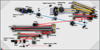 |
Fig. 2 3D CAO view of the SPEED test bed. Color code: telescope simulator and common path (orange), visible path (blue) and near-infrared path (red). Acronyms: TTM – tip/tilt mirror, OAP – off-axis parabola, ASM – active segmented mirror, DM – deformable mirror, FM – flat mirror, DIC – dichroic, L – lens, SCC-PS – self-coherent camera-phasing sensor, FPM – focal plan (mask), PIAA-M1 & PIAA-M2 – phase induced amplitude apodization mirror 1 & 2, LS – Lyot stop, NiR- near-infrared wavelengths, Vis. – optical wavelengths, FF – flip flop mirror, FW – filter wheel. The APCMC apodizer mask is located between the DM1 and DM2. In this configuration the PIAA-M1 and M2 are replaced by blank mirrors. |
3.2 The SPEED e2e model
SPEED e2e is a high-fidelity, end-to-end performance simulator of the bench, developed for specification, contrast analysis, and system verification (Beaulieu et al. 2018, 2020). The simulator incorporates Fresnel diffraction propagation using the PROPER library (Krist 2007), combined with a detailed and realistic system model (Martinez et al. 2023a), ensuring consistency with the latest bench optical design. It employs simulated wavefront sensing and control, integrating as-built optics with measured wavefront errors, and ensures that the emulator aligns with the SPEED bench optical contrast design.
The SPEED e2e reproduces the physical realities of optics positioning and wavefront errors on optical surfaces located far from the pupil plane. These effects, related to the Talbot length, introduce chromatic phase and amplitude perturbations via Fresnel propagation. Additionally, the simulator includes a dark hole generation algorithm that employs two out-of-pupil deformable mirrors (DM1 and DM2). This algorithm optimizes the zone of high contrast in the science image using a linear approach to minimize energy within the dark hole.
The dark hole algorithm is comprehensively detailed in other studies (Beaulieu et al. 2017, 2020; Martinez et al. 2024). Briefly, it begins by calculating the total energy at the image plane for a single deformable mirror, then generalizes to the case of two DMs. A setup matrix representation is used to compute the DM coefficients, which minimize energy within the dark region, referred to as the dark hole. The interaction matrix, representing the system’s response to each DM actuator, is derived by: (i) applying a small poke to each actuator, (ii) propagating the resulting wavefront through the optical setup, and (iii) recording the complex electric field at the focal plane.
The nominal e2e configuration, derived from the SPEED optical setup (Fig. 2), is illustrated in Fig. 3. This figure presents an in-line schematic of the e2e modeling and key assumptions. Pupil planes are marked with red lines, focal planes with red dots, and active optical elements are highlighted in green. Dotted lines (red or green) represent the protective windows of optical elements, appearing twice to account for the round-trip light propagation in the actual SPEED testbed, where optical propagation occurs in reflection. The e2e model includes 26 optical elements: an obscured mask with spiders mounted on a tip-tilt mirror (pupil mask); an imperfectly phased segmented mirror (ASM) with 163 segments including 3 missing segments (see Fig. 3, top map at the ASM plane), incorporating 5 nm RMS piston, 5 nm RMS tip/tilt, and 10 nm RMS focus errors (see Fig. 3, bottom map at the ASM plane); an APCMC coronagraph with a purpose-built focal plane mask (FPM, Martinez et al. 2020), a dedicated apodizer map (APOD, Sallard et al. 2024) manufactured and simulated in microdots, and a Lyot stop (LS) covering the area where segments are missing; and two deformable mirrors (DM1 and DM2) with 34 × 34 actuators, each with a finite stroke of 1.5 μm but infinite stroke precision, located 1.5 m and 0.2 m downstream of the pupil plane. The red circles over-plotted on the DM1 and DM2 surface indicate the beam footprint. All passive and active optics are assumed to have 5 nm RMS aberrations with a power spectral density proportional to f−3, except the dichroic and DM windows, which have 8 nm and 10 nm RMS aberrations, respectively. The total system aberration level is 30 nm RMS, consistent with the SPEED wavefront error after correcting NCPAs. The numerical pupil diameter is represented by 450 pixels, corresponding to a physical diameter of 7.7 mm on a 1024 × 1024 grid. The simulation is monochromatic at a wavelength of 1.65 μm.
To evaluate dOTF as a coronagraphic WFS, we simulated the inclusion of an additional DM, referred to as DM3, with characteristics identical to those of DM1 and DM2. Since the ASM is the only DM located in a pupil plane within the SPEED testbed, and a segment poke would introduce significant blurring in the dOTF estimates, DM3 was positioned in the sole available pupil plane, where SPEED’s PIAACMC M1 mirror is typically located. Consequently, PIAACMC M1 and M2 were replaced in the e2e with DM3 and a flat mirror, respectively. The baseline coronagraph used in the simulation is the APCMC, which employs the same focal plane mask (FPM) as the PIAACMC.
DM3 acts in the same way as a WFS by introducing a localized poke on an actuator near the edge of the pupil (see Fig. 3, top map at the DM3 plane, where the red dot on the top of the red circle marks the poked actuator). Furthermore, DM3 serves as a corrective element in NCPA correction tests. However, during cophasing and dark-hole digging operations, DM3 is used exclusively to generate the probe for the dOTF. The configurations of all DMs, based on the testing setup, are summarized in Table 1. In this context, active indicates that the DM is capable of adapting its shape, static refers to a state where the DM introduces a fixed pattern of wavefront errors, and flatten describes the scenario where the DM surface is flat, corresponding to its nominal map.
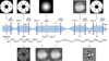 |
Fig. 3 In-line optical schematic design of the SPEED bench as implemented in the e2e emulator code. |
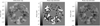 |
Fig. 4 Comparison of phase estimation in coronagraphic imaging mode using the dOTF conventional phase estimator (middle image) or the phase estimator derived under the small aberration regime (right image). The input phase map is provided in the left image. |
4 Numerical simulations
All simulations are monochromatic and the observing wavelength is 1.65 μm. For all testing setups (NCPAs, cophasing, dark-hole), a statistical analysis based on 128 different sets of aberration screen realizations is provided. The statistical validity of using 128 realizations has been verified in the context of dark-hole digging (Beaulieu et al. 2017), and, by extension, this approach is assumed to be valid for NCPAs and cophasing. Where applicable (NCPAs, cophasing), we compare the efficiency of dOTF in coronagraphic images with that in classical imaging, taking into account the off-axis PSF from our e2e code. When dOTF is applied in classical imaging mode, the phase can be estimated using either the conventional phase estimator (see Eq. (10)) or the one defined for the small aberration regime (Eq. (16)). Conversely, when dOTF is used in coronagraphic imaging mode, the phase or complex field can only be estimated using the estimator derived for the small aberration regime (e.g., Eq. (16), Eq. (18), or Eq. (19), depending on the intended application). The conventional phase estimator (Eq. (10)) is not applicable in this specific case. This limitation is illustrated in Fig. 4, which presents an example of a phase map (left image) introduced into our e2e simulation. The resulting phase estimated from coronagraphic images is compared when using the conventional estimator (middle image) and the estimator derived under the small phase approximation (right image). The results clearly demonstrate that the conventional estimator fails in this context, emphasizing the necessity of using the small aberration-based estimators in coronagraphic imaging scenarios. In practice, in all simulations concerned with dOTF in classical imaging, we use Eq. (16) for the sake of comparison with the coronagraphic mode.
For each testing set-up, we first highlight any relevant numerical assumptions or specific details, as well as the estimator used in practice. In all simulations, we compare the results obtained with the dOTF when the phase poke is applied using three different methods: a single pixel, an area of 5 × 5 pixels, or an actuator with a Gaussian influence function. The first two cases represent the use of a spatial light modulator (SLM), while the third case corresponds to a classical face-sheet deformable mirror, as modeled for DM1 and DM2.
Regarding the post-processing of the dOTF, only one of the two pupil fields present in the dOTF is considered and extracted. The overlap region, though limited, is not excluded from the analysis, although the information in this region is erroneous. We recall that it is possible to measure the complex field in the overlap region by using a second dOTF, where the poke is diametrically opposite to the one initially chosen, thereby enabling a reconstruction of the missing information. However, this goes beyond the scope of this study, which aims solely to demonstrate the capabilities of the dOTF in coronagraphic imaging. Therefore, the results presented represent a conservative estimate and define the lower bound of the achievable performance, although they can certainly be improved with further optimization. In addition, for NCPA and cophasing tests, global piston, tip and tilt are removed from the dOTF phase estimation prior to any correction.
For coronagraphs, we use an APCMC (currently in use in SPEED, Sallard et al. 2024) in all scenarios, with details of the FPM provided in the literature (Martinez et al. 2020). Although not explicitly shown in every case, all simulations were conducted using an APRC (apodized pupil Roddier coronagraph, Soummer et al. 2003), a PIAACMC (Guyon et al. 2014; Martinez et al. 2020, 2023b), and a vortex coronagraph (OVC, Foo et al. 2005). The APCMC and APRC coronagraphs offer similar advantages in the context of our NCPA and cophasing simulations. In our simulations, their Lyot stops are identical and can closely match the entrance telescope aperture, resulting in no modification of the FoV nor angular resolution, and thus Strehl ratios (a metric used in NCPA simulations) can be compared between the two situations. With a SPEED-like pupil, the OVC requires an aggressive Lyot stop. The PIAACMC, due to the PIAA unit, alters the entrance pupil diameter and central obscuration ratio by modifying the light ray distribution. For these coronagraphs, factors such as Strehl ratio evaluation, the effective number of actuators per DM, phase map projection onto DM3, localization of DM3, dOTF post-processing adaptations due to a reduced pupil field, and adjustments to poke localization must all be carefully adapted. To avoid adding unnecessary complexity to the system description and implementation, we restrict our presented results to the APCMC and APRC for NCPA and cophasing simulations, and to the APCMC only for the dark hole digging test series. However, in Appendix C, we provide a comparative dark hole result involving the APCMC, APRC, and PIAACMC.
Testing configurations and corresponding states of deformable mirrors.
4.1 Non-common path aberrations
For the NCPA tests, the dOTF phase estimator defined in Eq. (16) is used for both non-coronagraphic and coronagraphic images. In this configuration (see Table 1), DM3 is used to introduce the probe for the dOTF WFS and as the corrective system, while DM1 and DM2 remain flattened. The ASM exhibits no piston, tip/tilt misalignments in this test series, but missing segments are included. To simplify the situation, NCPA errors are introduced using a single phase map in the ASM plane (pupil plane), while all other optics are free of the 5 nm RMS aberrations described in the previous subsection. This approach avoids phase-amplitude mixing issues and eliminates the need for multiple DMs during correction. Since DM3, installed in a pupil plane, is the only DM used for this series of tests, it can only correct phase errors at that plane. A more complex scenario (see Section 4.3), involving both NCPAs correction (wavefront flattening) and wavefront shaping (dark hole creation), will introduce phase errors across all optics, most of which are not located in a pupil plane. In addition, during the correction, the phase measured by the dOTF is projected onto DM3. Since DM3 is a 34 × 34 element DM, with 27 elements spanning the beam diameter, the phase map is first projected and resampled using interpolation onto this reduced number of samples. The resized map is adjusted to account for the actuator influence function, determining the actuator heights required to achieve the desired surface profile.
In Fig. 5, our results are displayed as histograms showing the Strehl ratio (expressed as a percentage) as a function of the number of evaluations performed across 128 statistically independent NCPA realizations. In all plots, the red-dot histograms represent the initial Strehl ratio due to NCPAs before dOTF estimation and correction. The first series of tests assume 100 nm RMS NCPAs (Strehl ratio ranging from 85 to 88%), illustrated in the top left, top right, and bottom left histograms. The second series assumes 50 nm RMS NCPAs (Strehl ratio of ~96/97%), represented in the bottom right histogram. Figure 5 (top left) shows the results obtained in classical imaging mode when the dOTF is performed with a phase modification of λ/10 over a single pixel (green), a 5 × 5 pixel area (blue), or using an actuator with an influence function (yellow) to introduce the pupil modification. In these cases, the improvement is clear, achieving a Strehl ratio of approximately 95% with limited dispersion among the scenarios. A similar analysis is conducted for the coronagraphic imaging mode, as illustrated in Fig. 5 (top right). The results are consistent with those from the classical imaging mode, with no significant differences observed. However, the dispersion between realizations is smaller in the coronagraphic mode, leading to more sharply peaked histograms.
Figure 5 (bottom left) compares the histograms for two different coronagraphic modes (using an APCMC and an APRC) with the classical imaging mode when the dOTF is performed using a phase modification of λ/10 over a single pixel. This test demonstrates that the dOTF technique is compatible with various coronagraphs. Furthermore, the NCPAs improvement observed in coronagraphic mode appears to be independent of the coronagraph type and is comparable to the results obtained in classical imaging mode. Finally, Fig. 5 (bottom right) presents the analysis conducted in a different NCPAs regime (50 nm RMS). In this case, the initial Strehl ratio is higher than in the previous scenarios, but the improvement remains observable. The results are consistent across different coronagraphs and between observing modes, further demonstrating the robustness of the dOTF technique. For illustration, Fig. 6 presents a set of images for a specific NCPAs realization, including the initial phase screen, the dOTF-estimated phase in coronagraphic imaging mode across various implementations (using 1 × 1 pixel, 5 × 5 pixels area or a DM3 actuator as a poke), and the corresponding phase map projected onto DM3 for correction. Additionally, it displays the initial PSF, the corrected PSF, and the ideal reference PSF without aberrations. All simulations were conducted in closed-loop operation, with no convergence issues observed. The analysis was limited to two estimation/correction iterations per scenario.
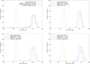 |
Fig. 5 Results of dOTF for NCPAs correction. The panels display Strehl ratio histograms measured before and after NCPAs estimation and correction. They correspond to: classical imaging in a relatively high-NCPAs regime (top left); coronagraphic imaging with various dOTF poke implementations (top right), coronagraph types (bottom left); and coronagraphic imaging in a low-NCPAs regime for different coronagraphs (bottom right). |
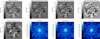 |
Fig. 6 Results of dOTF for NCPAs correction. The top row of panels shows the input phase map (top left), followed by phase maps estimated using different coronagraphic dOTF poke implementations from left to right. The second row sequentially presents the phase map projected onto DM3, the initial PSF, the corrected PSF, and the theoretically ideal PSF for reference. |
4.2 Fine cophasing
For the cophasing tests, the dOTF phase estimator defined in Eq. (16) is used on non-coronagraphic and coronagraphic images. In this configuration (see Table 1), DM3 is used only to introduce the dOTF probe, while DM1 and DM2 remain flattened. The ASM is used to introduce piston, tip/tilt misalignments and to correct them based on the phase analysis post-processed from the dOTF phase estimation. Because the goal of this series of test is to assess the ability of the dOTF to correct for cophasing errors in coronagraphic images, no NCPA errors are assumed, and all the optics are free from the nominal 5 nm RMS aberration level.
Simulations assume the ASM as the segmented hexagonal entrance pupil composed of 163 segments of 30 pixels width (corner to corner) over 7 hexagonal rings. We only consider in the test series, the segments where signal is not hidden by the 30% central obscuration or the edge of the circular pupil. To avoid secondary support to block all or part of the segment signals, we do not consider any secondary support in the entrance pupil. This simplified situation is meant to concentrate on the demonstration of the fundamental ability of the dOTF to operate on coronagraphic images. Dealing with signal partially hidden or biased is out of the scope of this study. Figure 7 (first and second images from the left) illustrates the SPEED entrance pupil along with the segments analyzed in this test series.
From the dOTF phase estimators (β, see Eq. (16)), the piston and tip/tilt values are directly extracted from the phase map using simple dedicated metrics (φ0, φ1, and φ2, for piston, tip, and tilt respectively). No interaction matrix is considered. For the estimation of the piston we calculate the integral of the dOTF phase map over a square zone (H) of side length h centered on each segment position defined by H, where x and y are the coordinate in the phase map plane. The estimator φ0 is expressed as
![Mathematical equation: $\[\varphi_{0}=\iint_{H} \beta \mathrm{~d} x \mathrm{d} y.\]$](/articles/aa/full_html/2025/08/aa55005-25/aa55005-25-eq21.png) (20)
(20)
For the estimation of the tip and tilt, the gradient of the signal β is estimated following the x and y axis respectively, and the estimators φ1 and φ2 are given by
![Mathematical equation: $\[\varphi_{1}=\iint_{H} \nabla_{x}[\beta] ~\mathrm{d} x \mathrm{d} y,\]$](/articles/aa/full_html/2025/08/aa55005-25/aa55005-25-eq22.png) (21)
(21)
![Mathematical equation: $\[\varphi_{2}=\iint_{H} \nabla_{y}[\beta] ~\mathrm{d} x \mathrm{d} y,\]$](/articles/aa/full_html/2025/08/aa55005-25/aa55005-25-eq23.png) (22)
(22)
where ∇x and ∇y stand for the gradient in the direction x and y respectively. Figure 8 compares histograms obtained in both coronagraphic and classical imaging modes for different dOTF poke implementations (using 1 × 1 pixel, 5 × 5 pixels area, or a DM3 actuator as a poke). The red-dot histograms represent the initial RMS values caused by the cophasing misalignment before dOTF estimation and correction. The tests assume an initial cophasing error of 45 nm RMS (comprising 50 nm RMS piston and 20 nm RMS tip-tilt errors). The analysis was limited to ten estimation/correction iterations per scenario, which was sufficient to reach the achievable correction threshold. In all cases, the process converges to small RMS residuals, with dOTF appearing more effective in coronagraphic imaging mode (residuals below 10 nm RMS) than in classical imaging (residuals below 20 nm RMS). Although the loss of resolution due to the spatial scale of the poke is observable (dispersion between histograms), its impact remains limited in coronagraphic mode and is more pronounced in non-coronagraphic imaging. In addition, Fig. 9 illustrates the histogram dispersion in coronagraphic imaging mode, distinguishing between piston and tip/tilt residuals. The probe convolution effect due to the probe spatial scale impacts the tip/tilt estimator more than the piston estimator as expected from classical imaging analysis (Dharmadhikari et al. 2024). Figure 7 (third and fourth images from the left) depicts an initial, un-phased ASM state alongside the final ASM configuration after dOTF fine cophasing, for illustrative purpose.
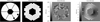 |
Fig. 7 Results of dOTF for cophasing correction. From left to right: the SPEED entrance pupil, the segments used for cophasing tests, an example of the initial ASM misalignment map, and the final ASM map after successive corrections in coronagraphic imaging mode. |
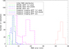 |
Fig. 8 Results of dOTF for cophasing correction. The panels show RMS error histograms measured before and after the final cophasing correction convergence. The histograms represent different scenarios, including classical imaging (dashed and dotted lines) and coronagraphic imaging (dashed lines), using various dOTF poke implementations. |
4.3 Dark hole digging
In this section, we evaluate the capability of the dOTF to operate as a WFS for wavefront shaping, specifically for creating a dark hole. The term “dark hole digging” refers to increasing the contrast within a specific FoV in a coronagraphic image. Consequently, this series of tests exclude the evaluation of dOTF in conventional imaging mode for comparative purposes, as was performed for NCPA and cophasing tests. For dark hole digging, all passive and active optics exhibit 5 nm RMS aberrations with a power spectral density proportional to f−3, except the dichroic and DM windows, which have 8 nm and 10 nm RMS aberrations, respectively, leading to a total system aberration level of ~30 nm RMS, and cophasing errors (5 nm RMS piston, 5 nm RMS tip/tilt, and 10 nm RMS focus errors) are considered. The e2e setup configuration reflects all the assumptions presented in Sect. 3 and in Fig. 3. The dOTF poke used in practice was set to an amplitude of λ/20. In this configuration (see Table 1), DM3 is used exclusively to introduce the dOTF probe and remains flattened otherwise, while DM1 and DM2 are actively employed for wavefront shaping. The ASM introduces static piston and tip/tilt misalignments but does not participate in their correction. Since dark hole digging requires the full complex focal plane electric field, the dOTF estimator used is the one defined in the image plane with Eq. (19) (combining α and β estimators), derived from its initial pupil plane formulation (Eq. (18)). DM3 serves to generate the dOTF probe throughout the dark hole digging process and for estimating the complex field at the detector plane for building the interaction matrix required in our algorithm (see Beaulieu et al. (2017, 2020); Martinez et al. (2024) for more details). Our test setup (SPEED e2e) is specifically designed with DM1 and DM2 positioning on the bench to create a dark hole in a small FoV at small angular separations (Beaulieu et al. 2017). In our work, the dark hole characteristics are those specifically tailored to the SPEED testbed, our testing environment, but the dOTF technique remains compatible with other dark hole configurations, as long as they are managed by the wavefront controller and DMs optical configuration. As a result, our dark hole evaluation is constrained to the range between 1 and 4 λ/D. For comparison, the results obtained with dOTF are compared with those from an ideal, unrealistic WFS that perfectly measures the complex field at the detector plane.
Figure 10 displays examples of dark holes: the leftmost panel shows the dark hole produced by a perfect WFS, while the other panels show those obtained using dOTF with various poke implementations, ranging from a 1-pixel poke to a DM3 actuator poke (rightmost panel). The dark hole created with the ideal WFS yields an unrealistic contrast below the numerical noise floor, while the other implementations reach more realistic contrast levels. The key takeaway from Figure 10 is that dark holes can be effectively generated using dOTF as a wavefront sensor. Figure 11 presents the median contrast ratio histograms obtained using dOTF with various poke implementations (1 × 1 pixel, 5 × 5 pixel area, or a DM3 actuator as the poke). Using the dOTF WFS with a 1-pixel poke (green dashed line) yields contrast ranging from 10−9 to 10−10, while a loss of contrast is observed as the spatial scale of the probe increases. However, in the case of the actuator poke (purple dashed line), the contrast remains at a deeper level around 10−8. It is important to note that the overlap region of the dOTF map, where the information is corrupted, is neither excluded nor estimated using a different dOTF. Nevertheless, this does not prevent the dark hole algorithm from converging and achieving deep contrast. Some divergence in the statistics from 128 realizations is observed for the 5 × 5 pixel poke case, where, in a few instances, the contrast is limited to 10−6 or 10−7 levels. As the spatial scale of the probe increases, we observe a greater number of iterations required for the dark hole to converge. This issue stems from two factors: the blurring effect and the wider overlap and corrupted region in the complex field estimation, neither of which are corrected for, although they could be to some extent.
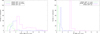 |
Fig. 9 Results of dOTF for cophasing correction. The panels display RMS error histograms measured before and after the final cophasing correction convergence. The left and right plots separately illustrate piston and tip/tilt residuals in coronagraphic imaging across different dOTF poke implementations. |
 |
Fig. 10 Results of dOTF for dark hole generation. From left to right: the dark hole image obtained using a perfect, ideal WFS, followed by the dark hole generated using dOTF WFS with various poke implementations. |
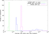 |
Fig. 11 Results of dOTF for dark hole generation. The panel displays the median contrast ratio histograms within the dark hole across different dOTF poke implementations. |
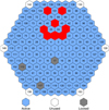 |
Fig. 12 SPEED ASM segment indexing with active, unused, and locked segments, where the segments in red are segments poked to create a smiley-like pattern for testing purpose. |
5 Laboratory experiments
In this section, we present a series of laboratory tests conducted on the near-infrared arm of the SPEED testbed (see Fig. 2) to experimentally validate the numerical results from the previous section. In SPEED, the coronagraph used is the APCMC, as our PIAACMC is awaiting a new generation of M1/M2 mirrors. The ASM is the only DM positioned in a pupil plane, which can be used to create the dOTF probe. This configuration imposes certain limitations on the scope of the tests, with the results constrained by the resolution loss caused by using a single segment as the poke entity. All tests were conducted in H-band (λ = 1650nm, BW = 3 nm), and the poke involved in the dOTF estimation in coronagraphic images is of amplitude λ/10.
In classical imaging mode, the dOTF was successfully used for NCPAs correction (Martinez et al. 2022; Dharmadhikari et al. 2024). During the NCPAs calibration, the mask on the tip/tilt mirror (TTM) was removed, ensuring the pupil was free of central obscuration and secondary supports. This offline calibration configuration allowed wavefront measurements across the entire pupil (full-filled pupil) and restricted the segment used (segment 92, see Fig. 12 that shows the ASM segment indexing) as a poke to cover only a limited portion of the pupil surface (~1 / 163e). For coronagraphic dOTF, the combination of the real SPEED entrance telescope pupil, characterized by its large central obscuration and secondary supports, with the constraints imposed by the APCMC Lyot stop (including a 10% reduction in the entrance pupil’s external diameter, a 10% increase in the central obscuration diameter, and a 20% increase in spider thickness) leads to an overall pupil surface reduction of 32%. Consequently, the poked segment occupies a larger fraction of the remaining pupil surface in this configuration. This leads to a pronounced blurring effect, which is significant and limiting in achieving precise wavefront estimation. In practice, the dOTF on SPEED in coronagraphic mode imaging is primarily limited to qualitative tests, as quantitative tests are not feasible.
A simple principle validation test is presented in Fig. 13. This test involves applying a uniform poke to several adjacent segments to create a recognizable (smiley) pattern without ambiguity. Eight segments were actuated with a piston of amplitude (λ/4). Figure 13 (left) shows the phase estimated in classical imaging using the estimator from Eq. (10), where a clear correspondence is observed between the applied pattern on the ASM mirror and the phase measurement obtained by the dOTF. Figure 13 (middle left) presents the same measurement using the same estimator but in coronagraphic imaging mode. In this case and as expected, the estimator suffers from sign ambiguities and fails to retrieve the phase correctly. Figure 13 (middle right) shows the phase estimated using the β estimator (Eq. (16)), where the smiley pattern is recovered. Notably, the differences in the pupil between this image and the left image arise from the application of the APCMC Lyot stop. Additionally, in Fig. 13 (right), the measurement obtained using the α estimator from Eq. (17) is also shown. These initial experimental results confirm that the classical phase estimator fails to provide meaningful information in coronagraphic imaging mode, while the small-phase approximation estimators offer a qualitatively accurate reconstruction of the complex field. Another simple principle validation test is presented in Fig. 14. This time we applied individual segment pokes of amplitude λ/10 and λ/20, each time with opposite signs. The objective of this test is to confirm that the sign changes are adequately retrieved by the dOTF in coronagraphic imaging mode. Figure 14 left and middle left images present the estimation using the β estimator from Eq. (16) for a λ/10 poke, negative (left) and positive (middle left). A similar result is presented in Fig. 14 middle right and right images but for a λ/20 segment poke. In all cases, the phase introduced by the segment poke as well as the sign change is correctly recovered. In terms of amplitude, the estimator yields values of approximately 115 nm and 130 nm for negative and positive pokes of λ/10 (165 nm), respectively, and 90 nm and 75 nm for negative and positive pokes of λ/20 (82.5 nm), respectively. In Fig. 15, we compare azimuthally averaged radial profiles of the off-axis PSF (black curve) with two APCMC profiles. The first APCMC profile (red curve) corresponds to the raw measurement when NCPAs are corrected by applying an offset map to the ASM, where this offset map was obtained using the dOTF WFS in a classical imaging scenario (APCMC FPM off-axis, no APCMC Lyot stop, and no SPEED entrance pupil, i.e., a full-field pupil). The second APCMC profile (blue curve) represents the result after a secondary NCPAs correction, based on a dOTF measurements in a coronagraphic imaging mode (with the APCMC). While the improvement is limited, an observable contrast enhancement occurs at angular separations close to the star’s center. In practice, the estimated phase is first projected onto Zernike polynomials, followed by an analytical decomposition into Zernike and hexagonal modes, which are then applied to the ASM (where three segments are not responding) over a hexagonal segmented optical aperture.
6 Conclusions
In this paper, we extended the application domain of the dOTF from classical imaging to high-contrast imaging. Specifically, we proposed an extension of the dOTF for estimating the complex field in coronagraphic images, employing either separate or joint phase and amplitude aberration estimators. Our study explored complex numerical simulations under realistic conditions and assumptions, with results supported by preliminary experimental data obtained from the SPEED testbed. Although these experimental results were primarily qualitative due to the limitations of the test apparatus, such as the large spatial scale of the probe and the use of the ASM, a segmented deformable mirror, as both a dOTF WFS and wavefront corrector, they nonetheless provided empirical validation of dOTF wavefront sensing ability in coronagraphic imaging mode.
Our NCPAs and cophasing simulation runs demonstrated the ability of dOTF to accurately estimate the phase using the β estimator (Eq. (16)) with coronagraphic images. Additionally, dark hole digging simulations showed that dOTF effectively estimates both phase and amplitude aberrations using the β (Eq. (16)) and α (Eq. (16)) estimators. Experimental data further supported these findings. The dOTF technique offers an effective and straightforward approach for complex field measurement in coronagraphic imaging, with the DM actively contributing to the process. By reducing the imaging workload, it presents a promising alternative to traditional coronagraphic WFS. Its demonstrated capability to estimate and correct NCPAs and segment misalignments, as well as its potential as a novel WFS for dark hole generation, highlights its significant value for high-contrast imaging applications.
In dark hole digging, two families of WFS (sensing algorithms) and WFC (control algorithms) associations exist, commonly referred to as model-based and model-free. These terms indicate whether a numerically simulated model of the optical system is required. For example, the PWP/EFC technique (Give’on et al. 2007b) is a model-based dark hole digging method that relies on an accurate model of the coronagraph. In contrast, the recent iEFC technique (Haffert et al. 2023; Ahn et al. 2023) merges WFS and WFC (PWP and EFC), providing a model-free alternative. Another commonly used model-free association is SCC (Baudoz et al. 2006) combined with EFC. In this broader framework of WFS and WFC, dOTF, which simplifies PWP (see Appendix B) and combined with EFC, has the potential to introduce yet another model-free approach to this landscape. With a single-actuator probe, the dOTF proves effective joint phase and amplitude wavefront sensing in coronagraphic imaging mode, without prior knowledge of the coronagraph type. In Appendix C, we show that a DH is obtained with various coronagraph types, with no prior information on the coronagraph design, when dOTF is used as a WFS in the DH digging process. dOTF offers an alternative to PWP, implementing a single-actuator to shape the probe and reducing the imaging workload during the sensing operation. The comparison between single-actuator PWP (Laginja et al. 2025) and single-actuator dOTF in terms of performance, contrast, convergence, sensitivity, and exposure times will be the subject of a forthcoming study and is beyond the scope of the present paper. However, Appendix D provides an initial assessment of the convergence and stability of the coronagraphic dOTF, both under nominal conditions and in scenarios where the small-aberration approximation breaks down due to higher levels of NCPAs.
An important expected advantage of dOTF lies in its ability to minimize the number of calibration probes, down to only one per complex field measurement, compared to at least three for traditional PWP-based methods. This reduction represents a system-level optimization that directly translates into more time available for scientific observations. In time-constrained missions such as the Nancy Grace Roman Space Telescope (Mennesson et al. 2022), where efficient use of observation time is critical, such optimization is particularly valuable. As demonstrated in (Laginja et al. 2025), even the choice of probe shapes can yield significant gains; dOTF may further enhance this efficiency by minimizing the number of probes needed. Moreover, iEFC, which relies on image differences rather than explicit focal-plane complex field measurements, indirectly exploits multiple dOTF-like signals without reconstructing the complex pupil field. This suggests that further adaptation is possible within iEFC itself, in addition to the promising potential of combining dOTF with EFC.
Finally, the extension of dOTF to high-contrast imaging has potential implications for both current and future telescopes, including the RST, large observatories, and laboratory testing during instrument integration and validation phases.
 |
Fig. 13 Experimental results of dOTF with the smiley pattern. From left to right: the phase map estimated using classical imaging (φ0 estimator), the phase map estimated using coronagraphic imaging with the classical phase φ0 estimator, the β estimator, and the α estimator. |
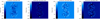 |
Fig. 14 Experimental results of dOTF in coronagraphic imaging mode using the β estimator when a single segment of the ASM is displaced up and down. From left to right: the phase map corresponding to a negative λ/10 poke, the phase map for a positive λ/10 poke, the phase map for a negative λ/20 poke, and the phase map for a positive λ/20 poke. |
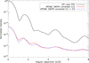 |
Fig. 15 Experimental results of dOTF. Azimuthally averaged radial profiles of the off-axis PSF (black curve) with two APCMC profiles: one when NCPAs are corrected using an offset map applied to the ASM, estimated in classical imaging mode (CLI, red curve), and another when the offset map applied to the ASM combines the one estimated in CLI with an additional correction estimated in coronagraphic imaging mode (CI, blue curve). |
Acknowledgements
The authors sincerely thank R. Soummer and E.H. Por for their valuable discussions and for introducing us to the dOTF concept, which contributed to the development of this work.
Appendix A Pairwise probing dOTF
Since the difference of the numerical Fourier transforms of images is equivalent to performing the numerical Fourier transform on the difference of the images, it is interesting to note that the dOTF can be rewritten such as,
![Mathematical equation: $\[\delta \mathcal{O}=\mathcal{F}^{-1}[\delta \mathcal{I}]=\mathcal{F}^{-1}\left[I_{1}-I_{0}\right],\]$](/articles/aa/full_html/2025/08/aa55005-25/aa55005-25-eq24.png) (A.1)
(A.1)
where I is the intensity image, I0 and I1 are intensity images where for one of them a pupil modification is introduced by an actuator probe. Following the idea proposed by Nguyen et al. (2023), an alternative implementation of dOTF exist, where we can take a difference of OTFs using opposite sign of pupil modification (positive/negative probe), Eq. (5) is expressed as
![Mathematical equation: $\[\delta \mathcal{O}=\mathcal{\mathcal{O}}_{1}^{+}-\mathcal{O}_{1}^{-},\]$](/articles/aa/full_html/2025/08/aa55005-25/aa55005-25-eq25.png) (A.2)
(A.2)
or equivalently as
![Mathematical equation: $\[\delta \mathcal{O}=\mathcal{F}^{-1}\left[I_{1}^{+}-I_{1}^{-}\right],\]$](/articles/aa/full_html/2025/08/aa55005-25/aa55005-25-eq26.png) (A.3)
(A.3)
which conceptually refers to PWP principle (Bordé & Traub 2006; Give’on et al. 2007b). Under this condition, Eq. (A.2) can further be rewritten as
![Mathematical equation: $\[\delta \mathcal{O}=2\left(\Psi_{s_{0}} \otimes \Psi_{D M_{probe}}^{*}+\Psi_{D M_{probe}} \otimes \Psi_{s_{0}}^{*}\right),\]$](/articles/aa/full_html/2025/08/aa55005-25/aa55005-25-eq27.png) (A.4)
(A.4)
where taking pairwise probe for the dOTF, the quadratic terms of Eq. (8) cancels, leaving just the two cross terms, whose magnitudes are doubled. The result presented in Eq. (A.4) was originally proposed by Nguyen et al. (2023) for increasing the dOTF signal-to-noise (S/N) and removing the cross terms.
However, we note that in real-life setups, additional cross terms still exist. Indeed, with non-compact phase pupil modifications (e.g., segment or actuator poke), the introduced phase change is not entirely known, even if we have a good estimate of the movement of a test segment or actuator. The modification of the complex field at the actuator or segment location remains unknown, especially for segment pokes, where the initial piston and tip/tilt alignment are uncertain and suboptimal. This issue has been studied in Martinez & Dharmadhikari (2023) by adding an additional pupil modification term common to the two OTFs, resulting in an additional phase term denoted ΔΨDMprobe, which transforms the dOTF expression into a new one, denoted δ𝒪′. If we assume the classical dOTF form where
![Mathematical equation: $\[\delta \mathcal{O}=\mathcal{O}_{1}-\mathcal{O}_{0},\]$](/articles/aa/full_html/2025/08/aa55005-25/aa55005-25-eq28.png) (A.5)
(A.5)
the resulting modification in the dOTF expression is given by
![Mathematical equation: $\[\delta \mathcal{O}^{\prime}=\delta \mathcal{O}+\Psi_{D M_{probe}} \otimes \Delta \Psi_{D M_{probe}}^{*}+\Delta \Psi_{D M_{probe}} \otimes \Psi_{D M_{probe}}^{*},\]$](/articles/aa/full_html/2025/08/aa55005-25/aa55005-25-eq29.png) (A.6)
(A.6)
where δ𝒪 is the classical dOTF expression as proposed in Eq. (8). Equation (A.6) shows two additional terms that are redundant, and it shows that the estimate of the electric field is subject to a phase offset corresponding to the unknown phase present at the poke location, that adds additional phase term to the dOTF. Now in PWP architecture applied to dOTF, where the dOTF form is modified to Eq. (A.2) the additional phase term remains, only δ𝒪 is expressed by Eq. (A.4) and not Eq. (8).
Appendix B Pairwise probing WFS and dOTF
Pairwise probing (Bordé & Traub 2006; Give’on et al. 2007b, 2011) uses pairs of DM probes of the same magnitude but opposite sign to modulate the electric field in defined regions of the science focal plane. Applying a predefined series of probe patterns to the DM surface, modulates the aberrated intensity distribution in the focal plane. Sinus cardinal functions probes were first proposed by Give’on et al. (2011), and more recently, various authors (e.g., Potier et al. 2020a; Haffert et al. 2023; Ahn et al. 2023; Milani et al. 2024; Laginja et al. 2025) use single-actuator probes as implemented in the dOTF, where recent studies advocate selecting the DM probes in its central area for PWP (Potier et al. 2020a; Haffert et al. 2023)) and the interest of single-actuator probe over sinc probes or other probe shapes (Laginja et al. 2025). Under these conditions, the intensity recorded by the science detector is:
![Mathematical equation: $\[I_{n}=\left|\psi_{s_{0}}+i \mathcal{C}\left[A \phi_{n}\right]\right|^{2},\]$](/articles/aa/full_html/2025/08/aa55005-25/aa55005-25-eq30.png) (B.1)
(B.1)
where 𝒞 is here the linear coronagraph operator, n is the index of the phase probe, and for each phase probe ϕn, a pair of images, denoted ![Mathematical equation: $\[I_{n}^{+}\]$](/articles/aa/full_html/2025/08/aa55005-25/aa55005-25-eq31.png) and
and ![Mathematical equation: $\[I_{n}^{-}\]$](/articles/aa/full_html/2025/08/aa55005-25/aa55005-25-eq32.png) are recorded, corresponding to probes ±ϕn. The difference between these images are computed so as
are recorded, corresponding to probes ±ϕn. The difference between these images are computed so as
![Mathematical equation: $\[I_{n}^{+}-I_{n}^{-}=4\left(\mathcal{R}\left[\psi_{s_{0}}\right] \mathcal{R}\left[i \mathcal{C}\left[A \phi_{n}\right]\right]+\mathcal{J}\left[\psi_{s_{0}}\right] \mathcal{J}\left[i \mathcal{C}\left[A \phi_{n}\right]\right]\right),\]$](/articles/aa/full_html/2025/08/aa55005-25/aa55005-25-eq33.png) (B.2)
(B.2)
The number of probes is, in practice, subject to a tradeoff between ensuring that Eq. (B.2) remains valid for all pixels of interest and minimizing overhead and impact during scientific acquisition. Considering k probes, the previous equation can be generalized and written for each pixel of the science detector with coordinates (i, j) as
![Mathematical equation: $\[\left[\begin{array}{c}I_{1}^{+}-I_{1}^{-} \\ \cdot \\ \cdot \\ \cdot \\ I_{k}^{+}-I_{k}^{-}\end{array}\right]_{(i, j)}=4\left[\begin{array}{cc}\mathcal{R}\left[i \mathcal{C}\left[A \phi_{1}\right]\right] & \mathcal{J}\left[i \mathcal{C}\left[A \phi_{1}\right]\right] \\ \cdot & \cdot \\ \cdot & \cdot \\ \cdot & \cdot \\ \mathcal{R}\left[i \mathcal{C}\left[A \phi_{k}\right]\right] & \mathcal{J}\left[i \mathcal{C}\left[A \phi_{k}\right]\right]\end{array}\right]_{(i, j)}\left[\begin{array}{l}\mathcal{R}\left[\psi_{s_{0}}\right] \\ \mathcal{J}\left[\psi_{s_{0}}\right]\end{array}\right]_{(i, j)}.\]$](/articles/aa/full_html/2025/08/aa55005-25/aa55005-25-eq34.png) (B.3)
(B.3)
To retrieve ψs0, at least two of the probes must induce different electric fields ψDM at a particular pixel location (i, j). For all pixels for which this condition is satisfied, Eq. B.3 can be inverted to estimate the real and imaginary parts of the electric field ψs0:
![Mathematical equation: $\[\left[\begin{array}{l}\mathcal{R}\left[\psi_{s_{0}}\right] \\ \left.\mathcal{J}\left[\psi_{s_{0}}\right]\right]_{(i, j)}\end{array}=\frac{1}{4}\left[\begin{array}{cc}\mathcal{R}\left[i \mathcal{C}\left[A \phi_{1}\right]\right] & \mathcal{J}\left[i \mathcal{C}\left[A \phi_{1}\right]\right] \\ \cdot & \cdot \\ \cdot & \cdot \\ \cdot & \cdot \\ \mathcal{R}\left[i \mathcal{C}\left[A \phi_{k}\right]\right] & \mathcal{J}\left[i \mathcal{C}\left[A \phi_{k}\right]\right]\end{array}\right]_{(i, j)}^{\dagger}\left[\begin{array}{c}I_{1}^{+}-I_{1}^{-} \\ \cdot \\ \cdot \\ \cdot \\ I_{k}^{+}-I_{k}^{-}\end{array}\right]_{(i, j)}\right.,\]$](/articles/aa/full_html/2025/08/aa55005-25/aa55005-25-eq35.png) (B.4)
(B.4)
where 𝒰† is the pseudo inverse of the matrix 𝒰 obtained from singular value decomposition method. Equation B.4 is made of state vector (the unknown to retrieve), a system matrix based on a numerical model of the instrument, and a measurement vector (difference of images).
It is noteworthy that the differential images from PWP is just one Fourier transform away from a series of dOTF images, because the difference of numerical Fourier transform of images is equivalent to performing the numerical Fourier transform of the difference of the images:
![Mathematical equation: $\[\mathcal{F}^{-1}\left[\left[\begin{array}{c}I_{1}^{+}-I_{1}^{-}\\\cdot \\\cdot \\\cdot \\I_{k}^{+}-I_{k}^{-}\end{array}\right]_{(i, j)}\right]=\left[\begin{array}{c}\delta \mathcal{O}_{1} \\\cdot \\\cdot \\\cdot \\\delta \mathcal{O}_{k}\end{array}\right]_{(i, j)}.\]$](/articles/aa/full_html/2025/08/aa55005-25/aa55005-25-eq36.png) (B.5)
(B.5)
Reformulating PWP (Eq. B.4) by projecting it into the Fourier domain enables solving the problem using differences of OTFs rather than differences of images. This approach enables the recovery of the pupil electric field instead of the focal plane electric field. These are two visions of the same problem. This is similarly equivalent, but this perspective emphasizes the fundamental physical similarities between dOTF and PWP, particularly considering their analogous probe application methods (positive/negative actuator pokes) discussed in the previous appendix. It also helps explain why dOTF is especially effective in coronagraphic imaging mode. In PWP, the image differencing method requires a complete and uniform speckle modulation across the entire field, necessitating generally at least three pairs of probes to recover the electric field, and is usually probing at actuators close to the center of the pupil (Potier et al. 2020a; Haffert et al. 2023; Laginja et al. 2025). When viewed in terms of OTF differencing, the overlap region, determined by such probe selection, is inherently broad, which, in turn, demands multiple probe pairs for accurate pupil field reconstruction. We recall that, in the dOTF, the field convolved with the probe and its conjugate, reflected about the origin, significantly overlaps due to the probe’s position in the pupil, as assumed in PWP.
dOTF WFS can be seen as a specific case of PWP, where PWP is simplified to operate with a minimal number of probe pairs. This simplification is achieved by favoring the actuator probe near the pupil edge, effectively isolating the pupil field and reducing the overlap region in the OTF domain (two diametrically opposite probe pairs can be combined to recover the information lost in the overlap region). Additionally, using a single-actuator probe, rather than alternative probe shapes, further minimizes this overlap (a single-actuator probe is conceptually closer to an ideal Dirac function). In this configuration, the PWP formalism, which involves reshaping the 2D electric and intensity fields into vectors and introducing an interaction or control matrix, becomes unnecessary. In this context, the advantage of dOTF becomes evident when considering the overhead associated with multiple probe pairs in PWP. Each additional probe pair requires two extra intensity images, increasing acquisition time and operational costs. While dOTF significantly reduces complexity, its efficiency relative to PWP remains an open question requiring further investigation.
Appendix C Dark hole, dOTF and coronagraphs
In this appendix, we extend the results presented in Sect. 4.3 to the case of DH digging, maintaining the same assumptions regarding the optical system, aberration level, number of DH realizations, etc., while varying only the coronagraph. The goal of this series of tests is to demonstrate that, without any prior knowledge of the coronagraph, high-contrast DH can still be achieved when using the dOTF as a coronagraphic WFS. We consider our APCMC configuration (as in Sect. 4.3) and compare it to an APRC and a PIAACMC (Guyon et al. 2014), designed for the SPEED testbed (Martinez et al. 2020, 2023b). To focus solely on the coronagraphic effects, we assume a dOTF WFS probe architecture using only a 1-pixel poke.
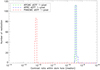 |
Fig. C.1 Results of dOTF for dark hole generation. The panel displays the median contrast ratio histograms within the dark hole across different coronagraph concepts. |
The APRC configuration closely resembles the APCMC; as shown in Fig. 3, the only modifications in the in-line schematic representation of the setup involve replacing the apodizer and FPM with those of the APRC. When using the PIAACMC, additional modifications are made to better match the actual SPEED design, as illustrated in Fig. 2. Specifically, no apodizer is used in the APOD plane, DM3 is removed from the pupil plane, and the PIAA M1 is installed. PIAA M2 is positioned 150 mm downstream from M1. The FPM remains the same as that of the APCMC, as the APCMC FPM reuses the one from the PIAACMC. DM3 is then reintroduced in the LS plane, and the PIAACMC Lyot stop is slightly shifted out of the pupil plane, as originally designed. DM3 could have been placed either in the pupil plane between DM1 and DM2 or in the LS plane. We opted for the LS plane since it is located downstream of the PIAA unit.
Figure C.1 presents the median contrast ratio histograms obtained using dOTF with the APCMC (green line), APRC (blue line) and PIAACMC (red line). Using the dOTF WFS with a 1-pixel poke yields contrast ranging from 10−9 to 10−10 (APCMC and APRC) and even deeper contrast with the PIAACMC. No divergence in the statistics from 128 realizations is observed in the data.
The reason why DH is deeper with the PIAACMC is not yet fully understood and will be the subject of a forthcoming study, which is beyond the scope of this paper. However, we can note that among these three concepts, the PIAACMC is the only one entirely optimized for the SPEED pupil (Martinez et al. 2020, 2023b), as the entire aperture architecture was considered in the optimization process of both the PIAA unit and the FPM. The APCMC, on the other hand, was introduced as a temporary solution while awaiting a new M1/M2 manufacturing campaign. As a result, the PIAA unit was redesigned as a pupil amplitude apodizer mask (Sallard et al. 2024). This was not an optimal design process, as it would have required re-optimizing all components, including the FPM. However, the APCMC retained the FPM of the PIAACMC. For the APRC, the optimization did not account for certain factors, such as the spider support structures. These factors may contribute to the observed discrepancies in achieved contrast.
Appendix D Stability and robustness of the dOTF
This section evaluates the convergence and stability of the coronagraphic dOTF under nominal conditions, followed by an analysis of its robustness when the small-aberration approximation breaks down due to larger NCPA levels.
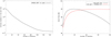 |
Fig. D.1 Convergence and stability as a function of iteration number. Top: Median contrast within the dark hole region during the dark hole digging process. Bottom: Evolution of the Strehl ratio during NCPAs correction. |
In the previous sections, the number of iterations required for convergence varies with the correction task and system configuration: typically 2 to 5 for NCPAs, around 10 for cophasing, and a few tens to hundreds for DH digging (see Fig. D.1, left panel). This depends on factors such as initial wavefront error, dOTF implementation (1-pixel, 5×5 pixels, or actuator-based), and loop gain.
A loop gain of 0.5 is used for NCPAs and cophasing, and is set to unity for DH digging. All loops include a progress-monitoring mechanism that halts iterations when no improvement is detected (for NCPAs and cophasing). DH optimization uses a two-level iterative scheme: first, it progressively includes singular values in the control matrix; then, for each subset, a sub-loop refines DM commands until contrast converges within ~10% of the theoretical value. If contrast stagnates or worsens, the loop reverts to the previous DM shape to avoid local minima caused by closely valued singular modes (Beaulieu et al. 2017).
To simplify the discussion, we focus on the long-term stability of the NCPAs correction loop. For moderate aberrations, convergence is typically fast and stable. However, in some cases (see Fig. D.1, right panel), the solution converges, briefly stabilizes and then diverges after several iterations (black curve). This behavior can be mitigated by reducing the loop gain or by introducing a leakage term, where the DM command at iteration i is a weighted combination of the current and previous commands. This limits the accumulation of systematic errors (red curve, Fig. D.1) that can lead to instability. These errors stem from effects such as unmasked overlap regions in the dOTF signal (that contains erroneous information and are not excluded in our dOTF post-processing), uncorrected blur from the poke’s spatial extent, errors from the interpolation required to project the dOTF-measured phase onto the lower-resolution DM3 actuator grid, and others. As noted in Section 4, the results represent conservative performance estimates that can be improved with dedicated optimization.
We also examine the behavior of the coronagraphic dOTF method when the small-aberration approximation is no longer valid. Specifically, we simulate cases with NCPA levels ranging from 165 to 550 nm RMS (roughly λ/10 to λ/3) using a 1-pixel dOTF. For simplicity, a unit loop gain, no leakage term, and a maximum of 25 iterations are used. Figure D.2 shows the resulting Strehl ratios as a function of iteration number for different NCPA levels (λ/3, λ/4, λ/5, λ/6, λ/8, and λ/10). The smalla-berration regime is considered valid below λ/6 (i.e., phase < 1 rad). Results show that while the estimation degrades outside the small-aberration regime, most notably for the pink and yellow curves (and likely others in terms of peak-to-valley metrics), the algorithm remains stable and does not diverge. Strehl improves in all cases, though for stronger NCPAs, only the PSF core is well reconstructed, while the wings remain uncorrected. The retrieved phase remains globally correlated with the input phase, although local errors, whose number and severity increase with the amount of NCPAs, limit further correction.
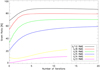 |
Fig. D.2 Convergence of NCPAs correction as a function of the input NCPAs amplitude. |
References
- Ahn, K., Guyon, O., Lozi, J., et al. 2023, A&A, 673, A29 [NASA ADS] [CrossRef] [EDP Sciences] [Google Scholar]
- Bailey, V. P., Bendek, E., Monacelli, B., et al. 2023, SPIE Conf. Ser., 12680, 126800T [NASA ADS] [Google Scholar]
- Baudoz, P., Boccaletti, A., Baudrand, J., & Rouan, D. 2006, in IAU Colloq. 200: Direct Imaging of Exoplanets: Science and Techniques, eds. C. Aime, & F. Vakili, 553 [Google Scholar]
- Beaulieu, M., Abe, L., Martinez, P., et al. 2017, MNRAS, 469, 218 [NASA ADS] [CrossRef] [Google Scholar]
- Beaulieu, M., Martinez, P., Abe, L., et al. 2018, SPIE Conf. Ser., 10700, 1070030 [Google Scholar]
- Beaulieu, M., Martinez, P., Abe, L., et al. 2020, MNRAS, 498, 3914 [NASA ADS] [CrossRef] [Google Scholar]
- Bordé, P. J., & Traub, W. A. 2006, ApJ, 638, 488 [Google Scholar]
- Codona, J. L. 2012, SPIE Conf. Ser., 8447, 84476P [Google Scholar]
- Codona, J. L. 2013, Opt. Eng., 52, 097105 [CrossRef] [Google Scholar]
- Codona, J. L., & Doble, N. 2015, J. Astron. Telesc. Instrum. Syst., 1, 029001 [NASA ADS] [CrossRef] [Google Scholar]
- Delorme, J. R., Galicher, R., Baudoz, P., et al. 2016, A&A, 588, A136 [NASA ADS] [CrossRef] [EDP Sciences] [Google Scholar]
- Dharmadhikari, R., Martinez, P., Gouvret, C., et al. 2024, SPIE Conf. Ser.,. 13097, 130973Q [Google Scholar]
- Foo, G., Palacios, D. M., & Swartzlander, G. A. 2005, Opt. Lett., 30, 3308 [NASA ADS] [CrossRef] [Google Scholar]
- Galicher, R., Baudoz, P., & Rousset, G. 2008, A&A, 488, L9 [NASA ADS] [CrossRef] [EDP Sciences] [Google Scholar]
- Galicher, R., Baudoz, P., Rousset, G., Totems, J., & Mas, M. 2010, A&A, 509, A31 [NASA ADS] [CrossRef] [EDP Sciences] [Google Scholar]
- Galicher, R., Potier, A., Mazoyer, J., et al. 2024, A&A, 686, A54 [NASA ADS] [CrossRef] [EDP Sciences] [Google Scholar]
- Give’on, A., Belikov, R., Shaklan, S., & Kasdin, J. 2007a, Opt. Express, 15, 12338 [Google Scholar]
- Give’on, A., Shaklan, S., & Kern, B. 2007b, in In the Spirit of Bernard Lyot: The Direct Detection of Planets and Circumstellar Disks in the 21st Century, ed. P. Kalas, 29 [Google Scholar]
- Give’on, A., Kern, B. D., & Shaklan, S. 2011, SPIE Conf. Ser., 8151, 815110 [Google Scholar]
- Guyon, O. 2004, ApJ, 615, 562 [NASA ADS] [CrossRef] [Google Scholar]
- Guyon, O., Hinz, P. M., Cady, E., Belikov, R., & Martinache, F. 2014, ApJ, 780, 171 [Google Scholar]
- Haffert, S. Y., Males, J. R., Ahn, K., et al. 2023, A&A, 673, A28 [NASA ADS] [CrossRef] [EDP Sciences] [Google Scholar]
- Herscovici-Schiller, O., Mugnier, L. M., Baudoz, P., et al. 2018, SPIE Conf. Ser., 10703, 1070329 [Google Scholar]
- Hinkley, S., Oppenheimer, B. R., Soummer, R., et al. 2007, ApJ, 654, 633 [NASA ADS] [CrossRef] [Google Scholar]
- Jiang, F., Ju, G., Qi, X., & Xu, S. 2019, Opt. Lett., 44, 4283 [NASA ADS] [CrossRef] [Google Scholar]
- Krist, J. E. 2007, Proc. SPIE, 6675, 66750P [NASA ADS] [CrossRef] [Google Scholar]
- Laginja, I., Baudoz, P., Mazoyer, J., et al. 2025, A&A, 698, A130 [NASA ADS] [CrossRef] [EDP Sciences] [Google Scholar]
- Malbet, F., Yu, J. W., & Shao, M. 1995, PASP, 107, 386 [NASA ADS] [CrossRef] [Google Scholar]
- Martinache, F. 2013, PASP, 125, 422 [NASA ADS] [CrossRef] [Google Scholar]
- Martinez, P. 2019, A&A, 629, L10 [NASA ADS] [CrossRef] [EDP Sciences] [Google Scholar]
- Martinez, P., & Dharmadhikari, R. 2023, A&A, 680, L12 [NASA ADS] [CrossRef] [EDP Sciences] [Google Scholar]
- Martinez, P., Kasper, M., Costille, A., et al. 2013, A&A, 554, A41 [NASA ADS] [CrossRef] [EDP Sciences] [Google Scholar]
- Martinez, P., Beaulieu, M., Barjot, K., et al. 2020, A&A, 635, A126 [NASA ADS] [CrossRef] [EDP Sciences] [Google Scholar]
- Martinez, P., Beaulieu, M., Gouvret, C., et al. 2022, SPIE Conf. Ser., 12184, 121843W [NASA ADS] [Google Scholar]
- Martinez, P., Beaulieu, M., Gouvret, C., Spang, A., & Marcotto, A. 2023a, The Messenger, 190, 55 [Google Scholar]
- Martinez, P., Beaulieu, M., Gouvret, C., et al. 2023b, A&A, 680, A6 [NASA ADS] [CrossRef] [EDP Sciences] [Google Scholar]
- Martinez, P., Beaulieu, M., Abe, L., et al. 2024, MNRAS, 532, 2892 [Google Scholar]
- Mazoyer, J. 2014, PhD thesis, Université Paris Diderot – Paris 7, France [Google Scholar]
- Mazoyer, J., Baudoz, P., Galicher, R., Mas, M., & Rousset, G. 2013, A&A, 557, A9 [NASA ADS] [CrossRef] [EDP Sciences] [Google Scholar]
- Mazoyer, J., Pueyo, L., N’Diaye, M., et al. 2018, AJ, 155, 8 [Google Scholar]
- Mennesson, B., Bailey, V. P., Zellem, R., et al. 2022, SPIE Conf. Ser., 12180, 121801W [NASA ADS] [Google Scholar]
- Milani, K., Douglas, E. S., Haffert, S. Y., & Van Gorkom, K. 2024, arXiv e-prints, [arXiv:2405.03899] [Google Scholar]
- Milli, J., Banas, T., Mouillet, D., et al. 2016, SPIE Conf. Ser., 9909, 99094Z [NASA ADS] [Google Scholar]
- Nguyen, M. M., Por, E. H., Sahoo, A., et al. 2023, in Techniques and Instrumentation for Detection of Exoplanets XI, 12680, SPIE, 834 [Google Scholar]
- Paul, B., Mugnier, L. M., Sauvage, J. F., Ferrari, M., & Dohlen, K. 2013a, Opt. Express, 21, 31751 [Google Scholar]
- Paul, B., Sauvage, J. F., & Mugnier, L. M. 2013b, A&A, 552, A48 [NASA ADS] [CrossRef] [EDP Sciences] [Google Scholar]
- Potier, A., Baudoz, P., Galicher, R., Singh, G., & Boccaletti, A. 2020a, A&A, 635, A192 [NASA ADS] [CrossRef] [EDP Sciences] [Google Scholar]
- Potier, A., Galicher, R., Baudoz, P., et al. 2020b, A&A, 638, A117 [NASA ADS] [CrossRef] [EDP Sciences] [Google Scholar]
- Potier, A., Mazoyer, J., Wahhaj, Z., et al. 2022, A&A, 665, A136 [NASA ADS] [CrossRef] [EDP Sciences] [Google Scholar]
- Pueyo, L., Kay, J., Kasdin, N. J., et al. 2009, Appl. Opt., 48, 6296 [NASA ADS] [CrossRef] [Google Scholar]
- Racine, R., Walker, G. A. H., Nadeau, D., Doyon, R., & Marois, C. 1999, PASP, 111, 587 [NASA ADS] [CrossRef] [Google Scholar]
- Sallard, C., Martinez, P., Spang, A., et al. 2024, SPIE Conf. Ser., 13097, 130976R [Google Scholar]
- Soummer, R., Aime, C., & Falloon, P. E. 2003, A&A, 397, 1161 [CrossRef] [EDP Sciences] [Google Scholar]
- Soummer, R., Pourcelot, R., Por, E. H., et al. 2024, SPIE Conf. Ser., 13092, 130921Z [Google Scholar]
- Vaughan, S. R., Gebhard, T. D., Bott, K., et al. 2023, MNRAS, 524, 5477 [Google Scholar]
All Tables
All Figures
|
Fig. 1 Conceptual drawing of the dOTF contents. |
| In the text | |
|
Fig. 2 3D CAO view of the SPEED test bed. Color code: telescope simulator and common path (orange), visible path (blue) and near-infrared path (red). Acronyms: TTM – tip/tilt mirror, OAP – off-axis parabola, ASM – active segmented mirror, DM – deformable mirror, FM – flat mirror, DIC – dichroic, L – lens, SCC-PS – self-coherent camera-phasing sensor, FPM – focal plan (mask), PIAA-M1 & PIAA-M2 – phase induced amplitude apodization mirror 1 & 2, LS – Lyot stop, NiR- near-infrared wavelengths, Vis. – optical wavelengths, FF – flip flop mirror, FW – filter wheel. The APCMC apodizer mask is located between the DM1 and DM2. In this configuration the PIAA-M1 and M2 are replaced by blank mirrors. |
| In the text | |
|
Fig. 3 In-line optical schematic design of the SPEED bench as implemented in the e2e emulator code. |
| In the text | |
|
Fig. 4 Comparison of phase estimation in coronagraphic imaging mode using the dOTF conventional phase estimator (middle image) or the phase estimator derived under the small aberration regime (right image). The input phase map is provided in the left image. |
| In the text | |
|
Fig. 5 Results of dOTF for NCPAs correction. The panels display Strehl ratio histograms measured before and after NCPAs estimation and correction. They correspond to: classical imaging in a relatively high-NCPAs regime (top left); coronagraphic imaging with various dOTF poke implementations (top right), coronagraph types (bottom left); and coronagraphic imaging in a low-NCPAs regime for different coronagraphs (bottom right). |
| In the text | |
|
Fig. 6 Results of dOTF for NCPAs correction. The top row of panels shows the input phase map (top left), followed by phase maps estimated using different coronagraphic dOTF poke implementations from left to right. The second row sequentially presents the phase map projected onto DM3, the initial PSF, the corrected PSF, and the theoretically ideal PSF for reference. |
| In the text | |
|
Fig. 7 Results of dOTF for cophasing correction. From left to right: the SPEED entrance pupil, the segments used for cophasing tests, an example of the initial ASM misalignment map, and the final ASM map after successive corrections in coronagraphic imaging mode. |
| In the text | |
|
Fig. 8 Results of dOTF for cophasing correction. The panels show RMS error histograms measured before and after the final cophasing correction convergence. The histograms represent different scenarios, including classical imaging (dashed and dotted lines) and coronagraphic imaging (dashed lines), using various dOTF poke implementations. |
| In the text | |
|
Fig. 9 Results of dOTF for cophasing correction. The panels display RMS error histograms measured before and after the final cophasing correction convergence. The left and right plots separately illustrate piston and tip/tilt residuals in coronagraphic imaging across different dOTF poke implementations. |
| In the text | |
|
Fig. 10 Results of dOTF for dark hole generation. From left to right: the dark hole image obtained using a perfect, ideal WFS, followed by the dark hole generated using dOTF WFS with various poke implementations. |
| In the text | |
|
Fig. 11 Results of dOTF for dark hole generation. The panel displays the median contrast ratio histograms within the dark hole across different dOTF poke implementations. |
| In the text | |
|
Fig. 12 SPEED ASM segment indexing with active, unused, and locked segments, where the segments in red are segments poked to create a smiley-like pattern for testing purpose. |
| In the text | |
|
Fig. 13 Experimental results of dOTF with the smiley pattern. From left to right: the phase map estimated using classical imaging (φ0 estimator), the phase map estimated using coronagraphic imaging with the classical phase φ0 estimator, the β estimator, and the α estimator. |
| In the text | |
|
Fig. 14 Experimental results of dOTF in coronagraphic imaging mode using the β estimator when a single segment of the ASM is displaced up and down. From left to right: the phase map corresponding to a negative λ/10 poke, the phase map for a positive λ/10 poke, the phase map for a negative λ/20 poke, and the phase map for a positive λ/20 poke. |
| In the text | |
|
Fig. 15 Experimental results of dOTF. Azimuthally averaged radial profiles of the off-axis PSF (black curve) with two APCMC profiles: one when NCPAs are corrected using an offset map applied to the ASM, estimated in classical imaging mode (CLI, red curve), and another when the offset map applied to the ASM combines the one estimated in CLI with an additional correction estimated in coronagraphic imaging mode (CI, blue curve). |
| In the text | |
|
Fig. C.1 Results of dOTF for dark hole generation. The panel displays the median contrast ratio histograms within the dark hole across different coronagraph concepts. |
| In the text | |
|
Fig. D.1 Convergence and stability as a function of iteration number. Top: Median contrast within the dark hole region during the dark hole digging process. Bottom: Evolution of the Strehl ratio during NCPAs correction. |
| In the text | |
|
Fig. D.2 Convergence of NCPAs correction as a function of the input NCPAs amplitude. |
| In the text | |
Current usage metrics show cumulative count of Article Views (full-text article views including HTML views, PDF and ePub downloads, according to the available data) and Abstracts Views on Vision4Press platform.
Data correspond to usage on the plateform after 2015. The current usage metrics is available 48-96 hours after online publication and is updated daily on week days.
Initial download of the metrics may take a while.