© The Authors 2025

1. Introduction

Interstellar magnetic fields play an important role in the structure and evolution of galaxies. They provide support to the gas against the gravitational field (Boulares & Cox 1990), affect the star formation rate (SFR; Tabatabaei et al. 2018; Krumholz & Federrath 2019) and the multi-phase structure of the interstellar medium (ISM; Ponnada et al. 2022; Gent et al. 2024), regulate galactic outflows and winds (Evirgen et al. 2019), and control the propagation of cosmic rays (CRs; e.g. Zweibel 2013).

Synchrotron radio emission is the best tool to study magnetic fields in the ISM. Synchrotron intensity depends on the strength of the field components in the sky plane and the number density of cosmic-ray electrons (CREs) in the relevant energy range. To measure the field strength, B, additional information about the CRE number density or a relation between B and the CRE number density is needed. Unpolarized synchrotron emission traces magnetic fields that cannot be resolved by the telescope beam, i.e. isotropic turbulent fields or ordered fields with orientations varying on scales smaller than the beam size. Linearly polarized synchrotron emission is a signature of the strength and orientation of resolved ordered fields in the sky plane; these can be regular fields or anisotropic turbulent fields.

Regular (‘mean’) fields, B_reg, are generated by the mean-field α–Ω dynamo (e.g. Beck et al. 1996; Chamandy 2016, Brandenburg & Ntormousi 2023, Chapter 7 in Shukurov & Subramanian 2021), reveal a coherent direction over several kiloparsecs. The mean-field dynamo generates azimuthal magnetic field modes that can be identified via large-scale variations in Faraday rotation measures (RMs; Table 5 in Beck et al. 2019).

Isotropic turbulent fields, B_turb, are generated by turbulent gas motions, the small-scale dynamo (e.g. Brandenburg & Subramanian 2005 and Chapter 6 in Shukurov & Subramanian 2021), and can reach an energy density of some fraction of the energy density of turbulence. Tangling of the regular magnetic field by turbulence also produces isotropic turbulent fields with an energy density similar to that of the regular field (Appendix A in Seta et al. 2018, Section 4.1 in Seta & Federrath (2020), and Section 13.3 in Shukurov & Subramanian 2021).

Anisotropic turbulent fields, B_an, can be generated from turbulent fields by shearing or compressing gas flows; for example, shear by differential rotation (Section 5 in Hollins et al. 2017) with a larger dispersion in azimuthal orientation, or compression by density-wave shocks with a larger dispersion along the shock front. Anisotropic turbulent fields reverse their sign on the scales of turbulence¹. The degree of anisotropy, δ, is computed as δ = (1 + B_an²/B_turb²)^0.5.

Both anisotropic turbulent and regular fields give rise to linearly polarized emission. To distinguish these two components, additional observations of the regular field are required, such as Faraday RM or Zeeman spectral line splitting. The latter can be observed in dense clouds in the Milky Way but not yet in external galaxies. Faraday rotation of the polarization angle of synchrotron emission increases with the square of the wavelength, the density of thermal electrons, and the average strength of the field components along the line of sight. The sign of RM gives the field direction. As RM is sensitive only to the regular field component along the line of sight, its component in the sky plane remains unknown. This fact hinders the construction of a 3D model of the large-scale regular field in a galaxy.

The Andromeda galaxy M 31 (NGC 224) is the nearest spiral galaxy at a distance of 780 kpc, inclined by 75° with respect to the sky plane (see Table 1 of Beck et al. (2020) for basic parameters). Thanks to its proximity, M 31 is particularly suited for investigating the properties of the ISM. The total and linearly polarized emissions are concentrated in a toroidal structure between radii of about 8 kpc and 12 kpc from the galaxy’s centre. This is the region with the highest density of cold molecular gas (Nieten et al. 2006), warm neutral gas (Brinks & Shane 1984; Braun et al. 2009; Chemin et al. 2009), warm ionized gas (Devereux et al. 1994), and dust (Gordon et al. 2006; Fritz et al. 2012), and it is the location of most of the present-day star formation (e.g. Tabatabaei & Berkhuijsen 2010; Rahmani et al. 2016).

The polarization surveys of M 31 at λ6.2 cm and λ11.1 cm observed with the Effelsberg 100–m telescope enabled us to calculate RMs, which were interpreted as a large-scale axisymmetric spiral (ASS) pattern of the regular field, which is regarded as the lowest mode excited by the mean-field (α–Ω) dynamo (Berkhuijsen et al. 2003). Combined with another polarization survey at λ20.5 cm observed with the Very Large Array (VLA) D-array and the Effelsberg telescope (Beck et al. 1998), a model of the large-scale magnetic field was constructed by Fletcher et al. (2004).

With the advent of more sensitive receivers, three new surveys of M 31 were conducted with the Effelsberg telescope at λ3.6 cm, λ6.2 cm, and λ11.3 cm with significantly improved sensitivities and map extensions (Beck et al. 2020). A survey of M 31 at λ4.5 cm (6.6 GHz) covering a large field of 2.4° ×3.1° was conducted by Fatigoni et al. (2021) with the 64–m Sardinia Radio Telescope (SRT).

This paper presents the data used for this work in Section 2. Section 3 discusses the diffusion of CREs. Section 4 presents the maps of magnetic field strengths. Section 5 shows the radial variation in field strengths. Section 6 compares the energy densities of the various components of the ISM in M 31, and Appendix A discusses the origin of Faraday depolarization.

2. Data

Our investigations are based on the radio continuum maps at λ3.6 cm (8.35 GHz) and λ20.5 cm (1.465 GHz) presented by Beck et al. (2020). The original resolutions are 83″ and 45″, respectively. Background sources with flux densities above 5 mJy at λ20.5 cm and above 1.2 mJy at λ3.6 cm were subtracted. The central source of M 31 was also subtracted. Both maps were smoothed to a common resolution of $1\stackrel{\prime }{.}5$. Furthermore, the map at λ6.2 cm (4.85 GHz) at 3′ resolution by Beck et al. (2020) was used for the regions where the λ3.6 cm map lacks large-scale emission.

The original map at λ20.5 cm revealed weak diffuse emission on scales larger than the map size at λ3.6 cm. This was removed by a subtraction of an overall base level of 0.3 mJy/beam.

2.1. Thermal–non-thermal separation

In order to obtain maps of non-thermal (synchrotron) intensity (NTH) at these frequencies, we subtracted maps of thermal emission (TH) from the maps of total emission (I). We used the thermal map at λ20.5 cm that Tabatabaei et al. (2013a) derived from the extinction-corrected Hα map of Devereux et al. (1994), smoothed to HPBW = $1\stackrel{\prime }{.}5$ and scaled to λ3.6 cm by (3.6/20.5)^0.1, assuming a thermal spectral index² of α_th = 0.1. The resulting map is shown in Figure 1. The average thermal contribution to the total flux density in the radial range 8–12 kpc is 45% at λ3.6 cm and 15% at λ20.5 cm.

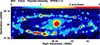Fig. 1. Thermal intensity of M 31 at λ3.6 cm with $1\stackrel{\prime }{.}5$ resolution. The rms noise is ≃0.3 mJy/beam. Contour levels are at 0.5, 1, 2, and 3 mJy/beam. Bright background sources have been subtracted.

2.2. Correction for anomalous microwave emission (AME)

The total spectral indices between λ3.6 cm and λ20.5 cm (Figure 13 in Beck et al. 2020) are smaller (flatter) than the total spectral indices between λ4.5 cm (6.6 GHz) and λ20.5 cm shown in Figure 12 of Fatigoni et al. (2021). Furthermore, the non-thermal spectral indices in Figure 14 of Beck et al. (2020) are smaller (flatter) than the non-thermal spectral indices between λ6.2 cm (4.85 GHz) and λ20.5 cm (Berkhuijsen et al. 2003).

One reason for this discrepancy could be a contribution of anomalous microwave emission (AME) by ultra-small dust grains (‘spinning dust’), as has been proposed by Fatigoni et al. (2021). From the AME flux density spectra of M 31 measured with low resolution by Fernández-Torreiro et al. (2024), referring to an integration area of 42 × 27 kpc, the flux density at 8.35 GHz is (0.44 ± 0.37) Jy, which is still an upper limit (Fernandez-Torreiro, priv. comm.). The large uncertainty arises from the not perfectly matching apertures, the different filtering techniques between instruments, different point source subtractions, and a possible contamination from the Galactic foreground. We measured a total flux density at λ3.6 cm of (1.41 ± 0.20) Jy over an integration area of 16 × 4 kpc (Beck et al. 2020), so that AME contributes less than 31% of the total flux density at λ3.6 cm.

In a pragmatic approach, we assumed that the spectrum of the synchrotron flux density integrated over the emission torus (between 8 kpc and 12 kpc radius) at 3′ resolution is constant between λ20.5 cm and λ3.6 cm. The non-thermal spectral index between λ20.5 cm and λ6.2 cm is 0.87 ± 0.01. To achieve the same non-thermal spectral index between λ20.5 cm and λ3.6 cm, the intensities at λ3.6 cm have to be reduced by 16.9 ± 0.5%. Assuming that the relative AME contribution is constant across the galaxy, we applied a correction factor of 0.831 to all non-thermal intensities at λ3.6 cm. The corrected map is presented in Figure 2 (top panel). As AME is not polarized, polarized intensities are not affected.

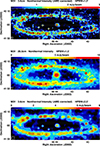Fig. 2. Non-thermal intensity of M 31 at λ3.6 cm with $1\stackrel{\prime }{.}5$ resolution (corrected for AME) (top), at λ20.5 cm with $1\stackrel{\prime }{.}5$ resolution (middle), and at λ3.6 cm with $2\stackrel{\prime }{.}5$ resolution (corrected for AME) (bottom). The rms noise is ≃0.25 mJy/beam (top), ≃0.25 mJy/beam (middle), and ≃0.4 mJy/beam (bottom). Contour levels are at 0.75, 1.5, 2.25, 3.0, and 4.5 mJy/beam (top), 2.5, 5.0, 7.5, 10, 15, 20 mJy/beam (middle), and 1.25, 2.5, 3.75, and 7.5 mJy/beam (bottom). The half-power beam widths are indicated in the bottom left corner. Bright background sources and the unresolved central source of M 31 have been subtracted. At λ3.6 cm, large-scale emission is missing in the central region.

The correction removes the discrepancy between the Effelsberg data at λ3.6 cm and the SRT data at λ4.5 cm (Fatigoni et al. 2021) only partly. We cannot exclude that the AME contribution is larger than estimated above. However, this should lead to a steepening in the synchrotron spectrum between λ6.2 cm and λ3.6 cm. The corresponding break in the CRE energy spectrum would need a synchrotron lifetime of CREs that is shorter than the residence time in the torus, which is not the case (see Section 3).

2.3. Final non-thermal maps

The emission from the toroidal structure between about 8 kpc and 12 kpc from the galaxy’s centre is clumpier at λ3.6 cm than at λ20.5 cm (Fig. 2). Strong emission emerges from regions with high SFRs evident from their Hα emission (Devereux et al. 1994), as discussed by Tabatabaei & Berkhuijsen (2010).

The central region of M 31 appears weaker at λ3.6 cm than at λ20.5 cm. The map at λ3.6 cm was combined from observations of seven small regions. Adjusting base levels when combining these regions was difficult and tended to suppress the extended emission. As a result, the diffuse total (and non-thermal) emission in the central region is weaker at λ3.6 cm compared to the maps at longer wavelengths that were observed in one single field. Consequently, the non-thermal intensities at λ3.6 cm within 8 kpc radius are not used in the following.

Figure 3 shows the radial variations in the average thermal, non-thermal, and polarized intensities at λ3.6 cm in the radial range 6–16.5 kpc. The uncertainties increase beyond 15 kpc radius. Fitting exponential functions I ∝ exp(−R/R_3.6) in the radial range 11–15 kpc gives scale lengths of R_3.6, th = (1.7 ± 0.2) kpc and R_3.6, nth = (2.7 ± 0.3) kpc. The non-thermal emission at λ20.5 cm with 3′ resolution (not shown here) was detected until 20 kpc radius with small uncertainties. The scale length in the radial range 11–20 kpc is R_20.5, nth = (3.1 ± 0.1) kpc.

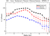Fig. 3. Radial variation in the intensities (in log scale) of the non-thermal (corrected for AME), thermal, and polarized emission at λ3.6 cm at $1\stackrel{\prime }{.}5$ resolution averaged in 0.5–kpc wide rings in the galaxy plane. In this and the following figures, the error bars show the 1-σ uncertainties.

2.4. Non-thermal (synchrotron) spectral index

The AME correction applied to the intensities at λ3.6 cm increases (steepens) all non-thermal spectral indices between λ3.6 cm and λ20.5 cm by a constant offset of 0.106 compared to Fig. 14 of Beck et al. (2020). Figure 4 (top panel) shows the radial variation in the average spectral indices between λ3.6 cm and λ20.5 cm between 6 kpc and 16 kpc radius. The steepening of α_n beyond 15 kpc radius is weaker than in Fig. 15 of Beck et al. (2020). The steep spectral index in the radial range 6–9 kpc is an artefact of missing diffuse λ3.6 cm emission in the central region (see above).

Fig. 4. Top: Radial variation in the average spectral index, αn, of the non-thermal intensities at $1\stackrel{\prime }{.}5$ resolution between λ3.6 cm (corrected for AME) and λ20.5 cm in 0.5–kpc wide rings in the galaxy plane. Middle: Radial variations in the average spectral index, αn, of non-thermal intensities at 3′ resolution between λ3.6 cm (corrected for AME) and λ20.5 cm as well as between λ6.2 cm and λ20.5 cm in 1–kpc wide rings in the galaxy plane. Bottom: Radial variations in the average degrees of polarization, pn, of the non-thermal intensities at λ3.6 cm (corrected for AME) and at λ6.2 cm, both at 3′ resolution, at λ11.3 cm at 5′ resolution, and at λ20.5 cm at 3′ resolution.

The average spectral indices between λ3.6 cm and λ20.5 cm and between λ6.2 cm and λ20.5 cm at 3′ resolution are compared in Figure 4 (middle panel). The agreement is good between 9 kpc and 13 kpc radius. The spectral steepening between λ3.6 cm and λ20.5 cm at smaller and larger radii could be due to energy losses (synchrotron and/or Inverse Compton) of CREs emitting at λ3.6 cm when propagating away from their places of origin in the torus at 8–12 kpc radius. Another reason could be that some large-scale emission is missing at λ3.6 cm due to the low signal-to-noise ratios outside the torus. Total intensity data at λ3.6 cm outside 8–12 kpc radius will not be included in the further analysis of this paper.

2.5. Polarization degree

Figure 4 (bottom panel) shows the average radial variation in the polarization degree p_n of non-thermal intensity, which is a measure of the degree of field order. p_n at λ6.2 cm remains roughly constant over the radial range 8–17 kpc. p_n at λ3.6 cm is similar, except for the radial range 8–9 kpc, which is affected by missing diffuse total intensity (see above). p_n at λ3.6 cm is somewhat smaller than p_n at λ6.2 cm beyond 15 kpc radius. Such a behaviour is hard to explain because p_n should decrease with increasing wavelength due to increasing Faraday depolarization. Some large-scale polarized emission at λ3.6 cm seems to be missing at large radii. Hence, polarization data at λ3.6 cm beyond 15 kpc radius will not be included in the further analysis. p_n at λ11.3 cm and λ20.5 cm are almost constant with radius, with lower percentages than at λ3.6 cm and λ6.2 cm, consistent with significant Faraday depolarization at those wavelengths.

3. Diffusion of cosmic-ray electrons

The map at λ20.5 cm shown in Figure 2 (middle panel) looks like a smoothed version of the map at λ3.6 cm, which is the result of CRE diffusion. The diffusion length in spiral galaxies has been estimated by various authors. By comparing the distributions of star formation surface density and radio continuum, Heesen et al. (2019) found diffusion lengths at λ22 cm of 1.0–3.4 kpc for three spiral galaxies. With a similar method, Vollmer et al. (2020) derived diffusion lengths at λ21 cm of 0.80–2.4 kpc for a sample of eight spiral galaxies. By comparing the distributions of the thermal and non-thermal emission components of M 31, Berkhuijsen et al. (2013) estimated a CRE diffusion length at λ20.5 cm of l_diff, 20.5 = (0.93 ± 0.21) kpc in the sky plane. Applying the method of wavelet cross-correlation between radio and far-infrared intensities, Tabatabaei et al. (2013b) derived l_diff, 20.5 = (0.73 ± 0.09) kpc in the sky plane.

The clumpiness of the emission torus at λ3.6 cm (Fig. 2, top panel) indicates that CRE diffusion does not play a significant role at this wavelength and this resolution, hence $l_{\mathrm{diff},3.6}\lesssim 1\stackrel{\prime }{.}5\equiv 0.34$ kpc in the sky plane. To measure the diffusion length at λ20.5 cm, we smoothed the λ3.6 cm map with Gaussian functions to resolutions increasing in steps of 15″ and correlated the intensities with the intensities at λ20.5 cm on linear and log scales, both above three times the noise levels, pixel by pixel. The highest Pearson correlation coefficient of 0.695 (linear/linear) and 0.675 (log/log) was found for the λ3.6 cm map smoothed to $2\stackrel{\prime }{.}5$. The map at $2\stackrel{\prime }{.}5$ (0.57 kpc) shown in Figure 2 (bottom panel) is most similar to the λ20.5 cm map at $1\stackrel{\prime }{.}5$ (Figure 2, middle panel). We conclude that the average CRE diffusion length at λ20.5 cm is l_diff, 20.5 ≃ 0.57 kpc in the sky plane, similar to the estimate by Tabatabaei et al. (2013b).

The diffusion length, l_diff, depends on the diffusion coefficient, D, and the CRE lifetime, τ, as l_diff = (D ⋅ τ)^0.53. If τ is limited by losses due to synchrotron emission or Inverse Compton scattering (τ ∝ E_CRE^− 1 ∝ λ^0.5), l_diff varies with wavelength λ as l_diff ∝ λ^0.250 for constant D, or l_diff ∝ λ^0.375 for an energy-dependent D ∝ E_CRE^0.5 (Strong 2007). Our estimates of l_diff, 20.5 ≃ 0.57 kpc and l_diff, 3.6 ≲ 0.34 kpc in the sky plane yield an exponent of the wavelength dependence of l_diff of ≳0.3, which is consistent with energy-dependent D and either synchrotron or Inverse Compton losses.

The corresponding diffusion coefficient is D = l_diff²/τ, where τ is the residence time of CREs emitting at λ20.5 cm in the torus. When assuming that τ is dominated by synchrotron losses, τ ≃ 5 ⋅ 10⁷ years in a magnetic field of ≃6.3 μG strength (see Section 4.1), we get D ≃ 2 ⋅ 10²⁷ cm²/s, much smaller than the values of D≃ (3–6) ⋅ 10²⁸ cm²/s favoured in models of CR propagation in the Galaxy (Moskalenko et al. 2002) and below the range of values derived for spiral galaxies of D≃ (1.4–8.9) ⋅ 10²⁸ cm²/s (Mulcahy et al. 2016; Heesen et al. 2019; Vollmer et al. 2020). This result seems to be in conflict with the expectation that CRE diffusion is faster in a galaxy with a strongly ordered field like that in M 31 (Tabatabaei et al. 2013b; Nasirzadeh et al. 2024). With a residence time of CREs in the torus of a few times shorter than their lifetime due to synchrotron losses, we would a achieve a diffusion coefficient typical to those in other spiral galaxies. Inverse Compton losses of CREs with the stellar radiation field in the emission torus of M 31 may play an important role and significantly reduce the CRE lifetime.

4. Magnetic field strengths in the emission torus

4.1. Strength of the total equipartition field

The synchrotron intensity, I_syn, scales with the density, N_CRE, of CREs in the energy range corresponding to the observation frequency and the total magnetic field strength, B_tot, ⊥, in the sky plane as I_syn ∝ N_CRE B_tot, ⊥^{(1 + α_n)}. If no independent information about N_CRE is available, for example from γ rays, a relation between N_CRE and B_tot is needed to find B_tot. A widely used assumption is that of equipartition between the energy densities of the total CRs and of the total magnetic field as developed by Beck & Krause (2005), with improvements by Arbutina et al. (2012).

Equilibrium between magnetic and cosmic-ray energy densities is reasonable at least on the scale of a large spiral galaxy because both quantities are closely related to the rate of star formation. Violation of overall equipartition may be caused by bursts of star formation or massive interaction with a neighbouring galaxy, both of which do not apply to M 31.

Seta & Beck (2019) argued that the equipartition assumption is not valid below scales of the CRE propagation length. In Section 3, we estimated an isotropic diffusion length at λ3.6 cm of l_diff, 3.6 ≲ 0.34 kpc, so that applying the equipartition assumption to our synchrotron map at this wavelength is reasonable.

The equipartition assumption yields N_CRE ∝ N_CR ∝ B_tot². In the ISM, protons dominate the total CRs. Hence, the CR energy density is determined by integrating over the energy spectrum of the protons. This allows us to calculate the total magnetic field strength from the synchrotron intensity, I_syn, according to Beck & Krause (2005):

$$\begin{array}{c}\hfill B_{\mathrm{tot},\perp }\propto {[I_{\mathrm{syn}}(K+1)/L_{\mathrm{syn}}]}^{1/(3+{\alpha }_{\mathrm{n}})},\end{array}$$(1)

where α_n is the synchrotron spectral index and L_syn is the effective pathlength through the synchrotron-emitting source. K is the ratio of number densities of CR protons and electrons in the relevant energy range. For diffusive shock acceleration of CRs in the ISM and moderate shock strengths, K ≃ 100 is a reasonable assumption in the energy range where the spectra of protons and electrons have a similar spectral index, i.e. beyond the rest-mass energy of protons (Bell 1978) and below the energy where losses of CR electrons become important.

The degree of non-thermal polarization, p_n, is needed for the geometrical correction to compute B_tot from B_tot, ⊥ (Beck & Krause 2005). As the equipartition strength is only a weak function of p_n, we used the average value of p_n = 18% at λ3.6 cm for the radial ring 8–12 kpc (see Figure 4, bottom panel) for all pixels in the map.

The emission torus of M 31 can be described by an elliptical profile with a full width, W, in the galaxy plane along the line of sight at 90° inclination and a full height, H, perpendicular to the galaxy plane. The pathlength, L, through the torus seen under the inclination angle, i, is

$$\begin{array}{c}\hfill L=H/{[1-{sin}^{2}i(1-{(H/W)}^2)]}^{0.5}.\end{array}$$(2)

The radial profile of synchrotron emission in Figure 3 yields a torus width of W_syn ≃ 4.5 kpc in the galaxy plane. This is also the pathlength through the torus along the line of sight on the minor axis at 90° inclination, which increases to about 15 kpc on the major axis. Berkhuijsen et al. (2013) found an exponential scale height of the non-thermal emission at λ20.5 cm of H_syn ≃ 0.33 kpc, which is significantly smaller than the average scale height of 1.4 kpc at λ20 cm for a sample of edge-on galaxies (Krause et al. 2018). The full height of 2H_syn ≃ 0.66 kpc means that the synchrotron-emitting torus of M 31 is flat (H_syn/W_syn ≪ 1) and Eq. (2) simplifies to L_syn = H_syn /cos i ≃ 2.5 kpc.

A pixel by pixel map of B_tot in the emission torus was computed from the maps at $1\stackrel{\prime }{.}5$ resolution of the total synchrotron intensities, I_syn, at λ3.6 cm (Fig. 2, top panel) and the spectral index map, α_n, between λ3.6 cm and λ20.5 cm (corrected for AME) that is reliable in the emission torus (8–12 kpc radial range). Only pixels were used where 0.53 ≤ α_n ≤ 1.4, which is the range where the equipartition assumption is applicable. For α_n < 0.53, corresponding to spectral indices ϵ of the CRE energy spectrum of ϵ < 2.06, the total CR energy density is dominated by the largest CRE energies, while for α_n > 1.4 or ϵ > 3.8, the CRE energy spectrum is dominated by synchrotron and/or Inverse Compton losses, so that K ≃ 100 is no longer valid (see Appendix in Heesen et al. 2023). We also discarded the central region of M 31 within 6 kpc radius for two reasons: the spectral index is uncertain in this region (see Fig. 4, top panel) and the pathlength is different from that through the emission torus.

Figure 5 (top panel) shows the strength of the total equipartition field, B_tot. The mean total field strength in the torus, averaged over sectors of 10° azimuthal width in the radial ring 8–12 kpc, is (6.8 ± 0.4) μG. Due to the nonlinear relation between total field strength and synchrotron intensity, this value is biased towards high peaks. The total equipartition field strength based on the mean synchrotron intensity and the mean synchrotron spectral index in the torus is more reliable and yields (6.3 ± 0.2) μG.

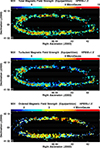Fig. 5. Maps of the strengths (in μG) of the total (top), isotropic turbulent (middle), and ordered magnetic fields in the sky plane (bottom) at $1\stackrel{\prime }{.}5$ resolution, computed from the total, unpolarized, and polarized non-thermal intensities at λ3.6 cm, assuming local equipartition between the energy densities of total magnetic fields and total CRs. Contour levels are at 7, 8, and 9 μG (total field and turbulent field), and 2.5, 3.5, and 4.5 μG (ordered field). Outside of the emission torus, synchrotron spectral indices are uncertain, so that no field strengths were computed.

The total field is decomposed into the isotropic turbulent field and the ordered field, B_tot² = B_turb² + B_ord². The ordered field has two components, the regular (mean) field and the anisotropic turbulent field, B_ord² = B_reg² + B_an². The strength of the isotropic turbulent field is estimated in Section 4.2, that of the ordered field in Section 4.3, that of the regular field in Section 4.6, and that of the anisotropic turbulent field in Section 4.7.

4.2. Strength of the isotropic turbulent equipartition field

Applying the equipartition assumption to the unpolarized intensity, I_unpol, emitted by CREs in an isotropic turbulent field, B_turb, ⊥, in the sky plane yields

$$\begin{array}{cc}\hfill I_{\mathrm{unpol}}& \propto N_{\mathrm{CRE}}{B}_{\mathrm{turb},\perp }^{(1+{\alpha }_{\mathrm{n}})}\hfill \\ \hfill & \propto B_{\mathrm{tot}}^2{B}_{\mathrm{turb},\perp }^{(1+{\alpha }_{\mathrm{n}})}\hfill \\ \hfill & \propto B_{\mathrm{turb}}^2{B}_{\mathrm{turb},\perp }^{(1+{\alpha }_{\mathrm{n}})}+B_{\mathrm{ord}}^2{B}_{\mathrm{turb},\perp }^{(1+{\alpha }_{\mathrm{n}})}.\hfill \end{array}$$(3)

As the degrees of polarization of non-thermal emission are relatively small, we may assume B_ord² ≪ B_turb², so that Equation (3) simplifies to

$$\begin{array}{c}\hfill I_{\mathrm{unpol}}\propto B_{\mathrm{turb}}^2{B}_{\mathrm{turb},\perp }^{(1+{\alpha }_{\mathrm{n}})},\end{array}$$(4)

with B_turb, ⊥² = 2/3 B_turb². Hence, the equipartition estimate can also be applied to derive the strength of B_turb from the unpolarized synchrotron intensity, I_unpol, which follows from

$$\begin{array}{c}\hfill I_{\mathrm{unpol}}=I_{\mathrm{syn}}-I_{\mathrm{pol}}/p_0,\end{array}$$(5)

where I_pol is the polarized intensity and p₀ is the intrinsic degree of polarization, p₀ = 73.5%, for the average non-thermal spectral index of α_n = 0.85.

Figure 5 (middle panel) shows the resulting map of B_turb. The equipartition strength based on the mean unpolarized synchrotron intensity in the torus is (5.4 ± 0.2) μG.

4.3. Strength of the ordered equipartition field

Finally, the linearly polarized emission, I_pol, is related to the ordered equipartition field strength B_ord, ⊥ in the sky plane:

$$\begin{array}{cc}\hfill I_{\mathrm{pol}}& \propto N_{\mathrm{CRE}}{B}_{\mathrm{orb},\perp }^{(1+{\alpha }_{\mathrm{n}})}\hfill \\ \hfill & \propto B_{\mathrm{tot}}^2{B}_{\mathrm{orb},\perp }^{(1+{\alpha }_{\mathrm{n}})}\hfill \\ \hfill & \propto B_{\mathrm{turb}}^2{B}_{\mathrm{orb},\perp }^{(1+{\alpha }_{\mathrm{n}})}+B_{\mathrm{ord}}^2{B}_{\mathrm{turb},\perp }^{(1+{\alpha }_{\mathrm{n}})}.\hfill \end{array}$$(6)

With B_ord² ≪ B_turb², Equation (6) simplifies to

$$\begin{array}{c}\hfill I_{\mathrm{pol}}\propto B_{\mathrm{turb}}^2{B}_{\mathrm{orb},\perp }^{(1+{\alpha }_{\mathrm{n}})}.\end{array}$$(7)

Equation (7) demonstrates that B_ord, ⊥ cannot be estimated from I_pol using the equipartition formula. Instead, B_ord, ⊥ can be computed via the relation B_ord, ⊥² = B_tot² − B_turb, ⊥². The resulting map is shown in Fig. 5 (bottom panel). The equipartition strength based on the mean polarized synchrotron intensity in the torus is (3.2 ± 0.3) μG.

4.4. Uncertainties in the equipartition field strengths

The equipartition field strengths, B, shown in Figure 5 are subject to various uncertainties:

(1) To be conservative, we assume that the parameters K and L_syn are known only to ≲50% accuracy, which leads to a total systematical uncertainty in B of ≲20%.

(2) The root mean square (rms) noise, σ, of the radio intensity maps causes statistical uncertainties. At the lowest level of 5σ the maximum uncertainty in B is ≃20%.

(3) Another statistical uncertainty emerges from that in α_n. An uncertainty of δα_n = 0.1 leads to an uncertainty in B of ≃7% for α_n = 0.7, ≃8% for α_n = 0.8, and ≃10% for α_n ≥ 1.0.

(4) The volume filling factor, f_syn, of synchrotron emission may be smaller than one, so that the pathlength, L_syn, has to be replaced by L_syn ⋅ f_syn, which increases the average total field strength, B_tot, ⊥.

(5) Fluctuations of B within the telescope beam and/or along the line of sight lead to an overestimate of the equipartition value. Due to the highly nonlinear dependence of I_syn on B_tot, ⊥ (Sect. 4.1), the average equipartition value ⟨B_tot, ⊥⟩ derived from synchrotron intensity is biased towards large field strengths and hence is an overestimate if B_tot varies along the line of sight and/or across the telescope beam (Beck et al. 2003).

For α_n = 1 and constant density of CRE (the non-equipartition case), the overestimation factor g of the total field is

$$\begin{array}{c}\hfill g={⟨B_{\mathrm{tot},\perp }^2⟩}^{1/2}/⟨B_{\mathrm{tot},\perp }⟩={(1+q^2)}^{1/2},\end{array}$$(8)

while for α_n = 1 and the equipartition case the overestimation factor, g, of the total field (Appendix A in Stepanov et al. 2014) is

$$\begin{array}{c}\hfill g={⟨B_{\mathrm{tot},\perp }^4⟩}^{1/4}/⟨B_{\mathrm{tot},\perp }⟩={(1+\frac{8}{3}{q}^2+\frac{8}{9}{q}^4)}^{1/4},\end{array}$$(9)

where ⟨  ⟩ indicates the volume average along the line of sight and across the beam, and q = ⟨δB_tot, ⊥²⟩^1/2 /⟨B_tot, ⊥⟩ is the amplitude of the field fluctuations relative to the average field. For extreme fluctuations of q = 1, the overestimation factor is 1.41 and 1.46 for the non-equipartition and equipartition cases, respectively. As equipartition is not valid on the spatial scale of field fluctuations, Equation (8) is the more realistic case.

The dispersion in B_tot in Figure 5 (top panel), determined in several regions of a few beam sizes extent, serves as an estimate of the 2D field fluctuations in the sky plane on the scale of our spatial resolution of 0.34 pc and is measured to be q_2D = 0.13 ± 0.02. Assuming isotropic turbulence yields q_3D = 3/2 q_2D = 0.20 ± 0.03 in 3D. As our spatial resolution is close to the largest scale of the Kolmogorov power spectrum of small-scale fields, the dispersion is representative for the total small-scale field (Amit Seta, private communication). q_3D ≃ 0.2 gives overestimation factors of g ≃ 1.02 and g ≃ 1.03 for the non-equipartition and equipartition cases, respectively.

The ratio, q_3D, is related to the volume filling factor, f_B, of the total field via

$$\begin{array}{cc}\hfill ⟨\delta B_{\mathrm{tot},\perp }^2⟩& ={⟨B_{\mathrm{tot},\perp }⟩}^2+⟨\delta B_{\mathrm{tot},\perp }^2⟩\hfill \\ \hfill & ={⟨B_{\mathrm{tot},\perp }⟩}^2/f_{\mathrm{B}},\hfill \\ \hfill f_{\mathrm{B}}=1/(q_{3\mathrm{D}}^2+1).\end{array}$$(10)

With q_3D ≃ 0.2, we get f_B ≃ 0.96. To our knowledge, this is the first estimate of the volume filling factor of the magnetic field in the diffuse ISM based on observations.

The Bayesian approach presented by Zychowicz & Chyży (2025) allows one to get a better handle on the uncertainties of the input parameters. A further development would be to allow curved radio spectra to be included.

4.5. Strength of the non-equipartition total field

The maps shown in Figure 5 are based on the assumption of equipartition at the scale of our spatial resolution of ≃0.34 kpc × 1.31 kpc in the galaxy plane along the major and the minor axis, respectively. The average diffusion length of l_diff, 20.5 ≃ 0.57 kpc, estimated in Section 3, indicates that the equipartition assumption is not valid at λ20.5 cm on the scale of our spatial resolution.

The CR diffusion is anisotropic (Chuvilgin & Ptuskin 1993; Yan & Lazarian 2004) and expected to be faster in a highly ordered magnetic field (Tabatabaei et al. 2013b; Nasirzadeh et al. 2024), like that in the emission torus of M 31. The diffusion length along the torus may well be larger than the average isotropic one of ≲0.48 kpc obtained in Section 3. Furthermore, Tharakkal et al. (2023a) concluded from their MHD model of the Parker instability that there are no signs of equipartition at kiloparsec scales. Signatures of Parker instabilities in M 31 were indeed observed (Beck et al. 1989).

In the following, we consider the extreme case of rapid CRE diffusion, ignoring energy losses and escape, resulting in constant CRE density along the torus, hence on a scale of several 10 kpc. Then, variations in I_syn are solely caused by variations in the total magnetic field strength, B_tot, ⊥:

$$\begin{array}{c}\hfill B_{\mathrm{tot},\perp }\propto {[I_{\mathrm{syn}}(K+1)/L]}^{1/(1+{\alpha }_{\mathrm{n}})}.\end{array}$$(11)

The non-equipartition map of B_tot (Figure 6) was computed from the maps of total intensities I_syn at λ20.5 cm (Fig. 2, middle panel) and the spectral index map α_n from Beck et al. (2020), corrected for AME. To calibrate the overall level of B_tot, ⊥, a minimal assumption was required, i.e. that equipartition is valid on average in the emission torus.

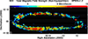Fig. 6. Map of the strength of the total magnetic field (in μG), determined from the total non-thermal intensities at λ20.5 cm at $1\stackrel{\prime }{.}5$ resolution, assuming global (but not local) equipartition between the energy densities of total magnetic fields and total CRs. Contour levels are at 7, 8, and 9 μG. The colour scale is the same as that in Fig. 5 (top panel).

The non-equipartition total field presented in Figure 6 shows larger variations compared to the equipartition total field (Fig. 5, top panel), as expected. The largest field strengths occur in star-forming regions with a maximum of 16.4 μG, compared to 10.6 μG for the equipartition field. This is illustrated in Figure 7 where equipartition and non-equipartition total field strengths are compared along azimuthal angle in the radial ring 8–12 kpc. The mean non-equipartition field strength in the torus, averaged in sectors of 10° azimuthal width in the ring 8–12 kpc, is (7.0 ± 1.0) μG, hence similar but with a larger dispersion compared to the equipartition field.

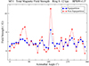Fig. 7. Variations in the strengths of the equipartition and non-equipartition total fields at $1\stackrel{\prime }{.}5$ resolution with azimuthal angle in the galaxy plane, counted from the north-eastern major axis in the sky plane (left side in Fig. 6), averaged in 10°–sectors of the radial ring 8–12 kpc.

4.6. Strength of the regular field

The ordered field, B_ord, ⊥, in the sky plane presented in Fig. 5 (bottom panel) has two components: the regular field, B_reg, ⊥, and the anisotropic turbulent field, B_an, ⊥. A separation of these two components is not possible based on polarized emission alone but needs additional data from RMs that are a tracer of regular fields along the line of sight. Faraday rotation is an ideal tool to study the structure of regular fields because it is insensitive to anisotropic turbulent fields. The mean-field dynamo generates large-scale modes of the regular field with spiral structures that are visible as large-scale RM patterns. Gas motions may tangle the regular field and distort the RM pattern. As is discussed in Beck et al. (2020), B_reg and B_an may have spiral structures with different pitch angles that are shaped by different physical processes.

In a perfectly ASS regular field, the basic (m = 0) dynamo mode, RM is expected to vary with azimuthal angle (Krause et al. 1989) as

$$\begin{array}{c}\hfill \mathrm{RM}={\mathrm{RM}}_{\mathrm{fg}}+{\mathrm{RM}}_{0}cos(\varphi -{\xi }_{\mathrm{reg}},\Vert ),\end{array}$$(12)

where RM_fg is the RM contribution from the Milky Way in the foreground of M 31, ϕ is the azimuthal angle in the galaxy plane, and the phase shift, ξ_reg, ∥, is the spiral pitch angle of the ASS field, expected to be constant along ϕ. RM₀ is the RM amplitude of the ASS mode near the north-eastern major axis of the projected emission torus, i.e. at the azimuthal angle ϕ = 0° +ξ_reg, ∥.

The variation in RM with azimuthal angle in the galaxy plane is close to sinusoidal (Beck 1982; Berkhuijsen et al. 2003; Beck et al. 2020). Figure 8 shows the average RMs at 3′ resolution in the radial ring 8–12 kpc. The cosine function gives an excellent fit to the data, yielding RM_fg = ( − 124 ± 5)  rad m⁻² and amplitude RM₀ = ( − 113 ± 10)  rad m⁻². The negative sign of RM₀ means that the regular field points away from us near the north-eastern major axis (azimuthal angle 0°).

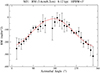Fig. 8. Variation in RMs between λ3.6 cm and λ6.2 cm at 3′ resolution with azimuthal angle in the galaxy plane, averaged in 10°–sectors of the radial ring 8–12 kpc, and fitted by a sinusoidal line (in red).

The pitch angle of ξ_reg, ∥ = −8° ±3° obtained from the fit is larger than that of −15° ±4° measured by Fletcher et al. (2004) for the radial range 9–13 kpc (at 780 kpc distance). The probable reason is that the method applied by Fletcher et al. (2004) is based on the position angles of the ordered fields, which are affected by anisotropic turbulent fields that have a smaller pitch angle (Beck et al. 2020) (see also Section 4.7).

The observed amplitude, RM₀, is given by

$$\begin{array}{c}\hfill {\mathrm{RM}}_0=0.5·0.812·B_{\mathrm{reg}}sini⟨n_{\mathrm{e}}⟩L_{\mathrm{th}},\end{array}$$(13)

where B_reg (in μG) is the volume-averaged strength of the regular field, i is the galaxy’s inclination, B_regsin i is the component, B_reg, ∥, of the average regular field along the line of sight, ⟨n_e⟩ is the average thermal electron density (in cm⁻³), and L_th (in parsecs) is the pathlength through the ionized medium. The factor 0.5 accounts for the fact that the observed average RM is smaller than the total RM from the far side of the emission region by this factor, assuming symmetric distributions of B_reg and ⟨n_e⟩ along the line of sight.

Equation (13) allows one to compute the strength of the regular field, B_reg, if L_th and ⟨n_e⟩ are known. An exponential scale height of the warm thermal gas of H_th, exp = (0.55 ± 0.1) kpc in the radial range 9–11 kpc (at 780 kpc distance) was obtained from fitting the Faraday depolarization data at λ6.2 cm and λ20.5 cm with 3′ resolution (Fletcher et al. 2004). We adopt a full thickness of H_th = (1.1 ± 0.2) kpc. The full width of the torus of thermal gas in the galaxy plane of W_th ≃ 3 kpc (Fig. 3) is smaller than that of the synchrotron emission, giving a pathlength through the torus at 90° inclination of 3 kpc on the minor axis and about 10 kpc on the major axis. The torus of thermal emission has a thicker profile than that of non-thermal emission. As the amplitude RM₀ is dominated by the pathlength around the major axis, H ≪ W is still valid, and, according to Eq. (2), the average pathlength at 75° inclination becomes L_th ≃ (4.25 ± 0.77) kpc.

⟨n_e⟩ is a quantity that is hard to measure. The typical emission measure (EM) of Hα emission from diffuse warm ionized gas in the torus of M 31 of 15 pc cm⁻⁶ (Walterbos & Braun 1994), a filling factor of 0.2, and the above pathlength of 4.25 kpc yields ⟨n_e⟩  ≃ 0.026 cm⁻³. Beck et al. (2019) estimated ⟨n_e⟩  ≃ 0.033 cm⁻³ from the total field strength B_tot based on the relation B_tot ∝ SFR^0.34 (Tabatabaei et al. 2017).

We applied a more direct method with the help of the thermal radio emission (Fig. 3), smoothed to 3′, the same resolution as the RM data. The thermal intensity, I_th (in mJy per beam), was transformed into the emission measure EM (in cm⁻⁶ pc) via (Ehle & Beck 1993; Dickinson et al. 2003):

$$\begin{array}{c}\hfill \mathrm{EM}=4.12I_{\mathrm{th}}{T}_{\mathrm{e}}^{0.35}{\nu }^{0.1}{\theta }^{-2}{a}^{-1}/1.08,\end{array}$$(14)

where T_e is the electron temperature (in Kelvin), ν is the observation frequency (in GHz), and θ is the telescope beamsize (in arcminutes). a is a correction factor depending on electron temperature and frequency (see Table 3 in Dickinson et al. 2003), and the factor 1.08 accounts for the contribution of helium atoms (Dickinson et al. 2003). We assume that T_e = (7000 ± 1000) K (see Fig. 1 in Tabatabaei et al. 2013b), θ = 3′, and a = 0.98. I_th = (2.02 ± 0.06) mJy/beam at ν = 8.35 GHz in the radial range 8–12 kpc yields EM = (24.0 ± 1.2) cm⁻⁶ pc, which is about twice larger than the average EM derived from Hα emission (Walterbos & Braun 1994) that is affected by absorption. Finally, ⟨n_e⟩ follows from

$$\begin{array}{c}\hfill ⟨n_{\mathrm{e}}⟩={(\mathrm{EM}{f}_{\mathrm{th}}/L_{\mathrm{th}})}^{0.5},\end{array}$$(15)

where L_th is the pathlength and f_th is the volume filling factor of the diffuse warm ionized gas. f_th was measured so far only in the Milky Way with help of pulsar dispersion measures and Hα emission measures. Berkhuijsen et al. (2006) found f_th = 0.05–0.3 at heights of 0–1 kpc from the mid-plane. Due to the lack of data on M 31, we adopt f_th = 0.20 ± 0.05. For the radial range 8–12 kpc, we obtain ⟨n_e⟩  = (0.034 ± 0.005) cm⁻³, similar to the previous estimates.

The strength of the regular field follows from

$$\begin{array}{c}\hfill B_{\mathrm{reg}}={\mathrm{RM}}_0/[0.5·0.812·sini{(L_{\mathrm{th}}\mathrm{EM}{f}_{\mathrm{th}})}^{0.5}].\end{array}$$(16)

With RM₀ = ( − 113 ± 10)  rad m⁻², Eq. (16) yields B_reg = (2.0 ± 0.5) μG. The uncertainty in B_reg includes the noise error in EM (from the noise error in I_th) and the systematic uncertainties in f_th and L_th. The radial variation in B_reg is discussed in Section 5.

4.7. Strength of the anisotropic turbulent field

To compute the anisotropic turbulent field, we subtracted the regular field in the sky plane from the observed ordered field in the sky plane. From Sect. 4.6 we know that the regular field is homogeneous along azimuthal angle in the radial range 8–12 kpc and has the strength B_reg.

The ASS regular field in the sky plane, B_reg, ⊥, varies with the azimuthal angle, ϕ, as

$$\begin{array}{c}\hfill B_{\mathrm{reg}},\perp =B_{\mathrm{reg}}|sin(\varphi -{\xi }_{\mathrm{reg}},\perp )|.\end{array}$$(17)

B_reg and ξ_reg, ⊥ ≃ ξ_reg, ∥ are taken from Section 4.6. The anisotropic turbulent field, B_an, ⊥, in the sky plane follows from

$$\begin{array}{c}\hfill B_{\mathrm{an}},\perp ={(B_{\mathrm{orb},\perp }^2-B_{\mathrm{reg}},{\perp }^2)}^{0.5}.\end{array}$$(18)

The azimuthal variations in B_ord, ⊥, B_reg, ⊥, and B_an, ⊥ are shown in Figure 9. The anisotropic field strength shows a similar variation with azimuthal angle, ϕ, as that of B_ord, ⊥, though with a lower amplitude. Averaging the ratio ⟨B_an, ⊥/B_ord, ⊥⟩ gives 0.84 with a low dispersion of 0.09. Hence, the ordered field is dominated by the anisotropic turbulent field. Around the minor axis (azimuthal angles ϕ ≃ 90° and ≃270°) B_reg, ⊥ is largest and almost reaches the level of B_ord, ⊥. As both quantities are measured with independent methods, this demonstrates that the equipartition assumption is reasonable.

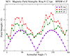Fig. 9. Variations in the strengths of the (plane-of-sky) ordered, axisymmetric (ASS) regular, and anisotropic turbulent fields at $1\stackrel{\prime }{.}5$ resolution with azimuthal angle, measured in the galaxy plane in the radial ring 8–12 kpc, using the spiral pitch angle of the ASS field of −8° taken from the fit shown in Fig. 8.

A phase shift between the variations in B_an, ⊥ and B_reg, ⊥ is obvious from Fig. 9. One reason could be deviations from a constant spiral pitch angle of the regular field, similar to what is observed for the gaseous spiral arms (Braun 1991; Nieten et al. 2006). The phase ξ_reg, ∥ of the RM variation in Fig. 8 is mostly constrained by the regions around the minor axis, while the phase ξ_reg, ⊥ in Fig. 9 is constrained by the regions around the major axis where the pitch angle may be different.

Furthermore, B_an and B_reg may have different average spiral pitch angles, as proposed by Beck et al. (2020), based on the different phases the variation in RM and of polarized intensity (their Table 6). A steeper pitch angle of ξ_reg, ⊥ ≃ −15° brings the peaks of B_an, ⊥ and B_reg, ⊥ closer together (Fig. 10).

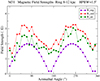Fig. 10. ariations in the strengths of the plane-of-sky ordered, axisymmetric (ASS) regular, and anisotropic turbulent fields at $1\stackrel{\prime }{.}5$ resolution with azimuthal angle, measured in the galaxy plane in the radial ring 8–12 kpc, assuming a spiral pitch angle of the ASS field of −15°.

The azimuthal variation in RM in Fig. 8 shows deviations from the fit, suggesting the existence of higher modes of the regular field with low amplitudes, e.g. the bisymmetric (BSS) dynamo mode superimposed onto the ASS mode, as suggested by Sofue & Beck (1987) and Beck et al. (2020). We allowed the fit to include the higher modes cos (2ϕ − ξ₂), cos (3ϕ − ξ₃), or cos (4ϕ − ξ₄) but none improved the fit significantly. The refined analysis by Paul et al. (2025) shows that several higher modes contribute to the pattern of the regular field in M 31.

Fig. 11 shows the variations in the isotropic turbulent field strength, B_turb, and the anisotropic turbulent field strength, B_an, ⊥, with azimuthal angle in the radial ring 8–12 kpc. The average strength of B_an, ⊥ is 2.0 μG with a dispersion of 0.5 μG. Applying the same bias correction as for B_ord, ⊥ (Sect. 4.3) yields (2.7 ± 0.7) μG. The average ratio ⟨B_an, ⊥/B_turb⟩ from Fig. 11 is 0.32 ± 0.10 or 0.50 ± 0.16 after correction for bias. The relatively small dispersion indicates that the generation of anisotropic turbulent fields is related to isotropic turbulent fields. As large-scale density-wave shock fronts are weak or missing in M 31, shearing by differential rotation is the probable origin of the anisotropy (Stepanov et al. 2014; Hollins et al. 2017).

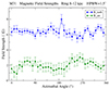Fig. 11. Variations in the isotropic turbulent field strength, Bturb, (Fig. 5, middle panel) and the strength of the (plane-of-sky) anisotropic turbulent field Ban, ⊥ (taken from Fig. 10) at $1\stackrel{\prime }{.}5$ resolution with azimuthal angle in the galaxy plane in the radial ring 8–12 kpc. The uncertainties in Bturb reflect the dispersion of the values in the map of Bturb in each sector. The uncertainties in Ban, ⊥ come from the dispersion of the values in the map of Bord, ⊥ (Fig. 5, bottom panel) in each sector and the general uncertainty of Breg, ⊥ as determined in Sect. 4.6.

5. Radial variations in magnetic field strength

Based on equipartition assumed to be valid on average within each radial ring of 1 kpc width in the galaxy plane, we computed the average strengths of the total, turbulent, and ordered fields at 3′ resolution as a function of radius. We used the average values of the non-thermal intensities at λ20.5 cm, of the non-thermal spectral index between λ6.2 cm and λ20.5 cm (Fig. 4, middle panel), and of the non-thermal degree of polarization at λ6.2 cm (Fig. 4, bottom panel). For the central region (0–3 kpc radius), we used a pathlength of L_syn = 0.5 kpc and an inclination of 43° (Gießübel & Beck 2014). For the radial range 3–20 kpc, we used the same inclination of 75° and pathlength of L_syn = 2.5 kpc as for the emission torus (Section 4.1). For the radial range 18–20 kpc, where the uncertainties are large, we used a constant non-thermal spectral index of 1.0 and a constant non-thermal degree of polarization of 17%.

The result is shown in Figure 12. The total and ordered fields peak at about 10 kpc radius, the turbulent field peaks at about 11 kpc radius, always followed by a slow decrease with increasing radius. Fits to the averages of total, turbulent, and ordered fields in the radial range 11–20 kpc by exponential functions B ∝ exp(−R/R₀) give similar scale lengths of R₀ = (14.1 ± 0.6) kpc, R₀ = (13.8 ± 0.4) kpc, and R₀ = (15.3 ± 1.4) kpc, respectively. Compared with the exponential scale length of the total non-thermal emission at λ20.5 cm at 3′ resolution of (3.1 ± 0.1) kpc (Section 2.2), the scale length of the total magnetic field is larger by a factor of 4.5 ± 0.2. This is consistent with the expectation from the assumption of energy equipartition for which a factor of (3 + α_n)≃4 is expected.

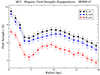Fig. 12. Average strengths (on a log scale) of the total, turbulent, and ordered fields at 3′ resolution in 1–kpc wide rings in the galaxy plane. The statistical uncertainties are assumed to be 10%. The systematical uncertainty of ≲20% (see Section 4.4) affects all values by the same amount and is not included.

Exponential scale lengths of the total equipartition field were estimated in five spiral galaxies by Basu & Roy (2013), with values ranging between 5 kpc and 18 kpc. Berkhuijsen et al. (2016) found a scale length in the outer disc of the spiral galaxy M 101 of about 20 kpc for the total and turbulent fields.

Profiles of the total magnetic field strength were determined for 198 analogues of the Milky Way and M 31 in the TNG50 simulation (Figure 19 in Pillepich et al. 2024). The average strength is 5 μG at 10 kpc radius and 3 μG at 20 kpc radius, similar to our observations (Fig. 12).

The radial variation in the strength B_reg of the regular field was obtained from the fit results of the sinusoidal azimuthal variation of RM between λ3.6 cm and λ6.2 cm at 3′ resolution in five rings between 7 kpc and 12 kpc (Beck et al. 2020). To estimate the densities of the diffuse warm ionized gas ⟨n_e⟩ in these rings with help of Equations (14) and (15), we measured the thermal intensities ⟨I_th⟩ in the same five rings from the map shown in Fig. 1, smoothed to 3′ resolution. We assumed the same constant pathlength through the warm ionized gas of L_th = 4.25 kpc and constant volume filling factor f_th = 0.2 (Section 4.6).

The strengths of the regular field, B_reg, in the five rings follow from Eq. (16), are listed in Table 1, and are shown in Figure 13. B_reg is on average smaller by about 40% than the equipartition strength of B_ord, ⊥ (containing regular and anisotropic turbulent fields). As B_reg and B_ord, ⊥ were measured with independent methods, this gives indication that the data are consistent with the equipartition assumption.

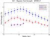Fig. 13. Average strengths (on a linear scale) of the turbulent and ordered fields (from Fig. 12) and of the regular field (Table 1) at 3′ resolution in 1–kpc wide rings in the galaxy plane. The uncertainties in Breg are estimated from the statistical uncertainties in RM and assuming a 5% uncertainty in ⟨ne⟩. The systematic uncertainties in Lth and fth of about 18% and 25%, respectively, affect all Breg values by the same amount and are not included.

Table 1 gives the strengths of the isotropic turbulent field B_turb, the ordered field B_ord, ⊥, and the anisotropic turbulent field B_an, ⊥ in the sky plane (derived from B_an, ⊥² = B_ord, ⊥² − B_reg²). The ratio B_reg/B_turb ≃ 0.39 is almost constant over all five rings. The ratio B_an, ⊥/B_turb ≃ 0.57 and the degree of anisotropy δ ≃ 1.15 are constant until 10 kpc radius and then decrease. Similarly, the ratio B_an, ⊥/B_ord, ⊥ ≃ 0.82 is constant until 10 kpc radius (similar to the average ratio in Fig. 10) and then decreases.

B_reg remains about constant in the radial range 7–12 kpc, while B_ord, ⊥ decreases (Fig. 13). If confirmed by future data at larger radii, possible reasons for this divergence are:

(1) The anisotropic turbulent field, B_an, ⊥, decreases radially faster than the regular field, B_reg, and gradually contributes less to the ordered field (see last column of Table 1). B_an, ⊥ decreases because the shear rate⁴ decreases with radius together with the gradient of angular velocity Ω, while the large-scale dynamo generating B_reg remains efficient until large radii.

(2) If the disc of warm thermal gas flares beyond about 10 kpc radius, as proposed by Fletcher et al. (2004), the pathlength L_th increases with radius and B_reg decreases with L_th^−0.5 (Eq. 16).

6. Energy densities

The dynamical importance of magnetic fields can be estimated by comparing the magnetic energy density with the thermal energy density of the diffuse warm ionized gas and the kinetic energy density of the turbulent neutral gas. We restricted our estimates to the emission torus at 8–12 kpc radius.

• The average equipartition strength of the total field in the emission torus (radial range 8–12 kpc) of 6.3 μG (Sect. 4.1) corresponds to a magnetic energy density of ϵ_mag ≃ 1.58 ⋅ 10⁻¹² erg cm⁻³. For a systematic uncertainty in B of ≲20%, the systematic uncertainty in ϵ_mag is ≲40%.

• To compute the kinetic energy density of the turbulent neutral gas, ϵ_kin, the mass density, ⟨ρ⟩, and the turbulent velocity, v_turb, need to be known. We computed a map of the column densities of the neutral gas from the HI and CO data (Braun 1991; Nieten et al. 2006) and measured N_gas ≃ 2.6 ⋅ 10²¹ cm⁻². The scale height of HI gas in the emission torus of H_gas ≃ 350 pc (Braun 1991), similar to the synchrotron scale height at λ20.5 cm (Sect. 4.1), yields a pathlength of L_gas ≃ 2.7 kpc and hence a volume density of the HI gas of ⟨n⟩  = 0.31 cm⁻³ and a mass density of ⟨ρ⟩  = 5.2 ⋅ 10⁻²⁵ g cm⁻³. Allowing for a helium contribution of ≃30% to the mass yields ⟨ρ⟩  = 6.8 ⋅ 10⁻²⁵ g cm⁻³. Caldú-Primo et al. (2013) measured a typical turbulent velocity of v_turb = 12 km/s for nearby spiral galaxies from spectral line observations that refers to one dimension. For three dimensions, we get ϵ_kin = 1.5 ⟨ρ⟩ v_turb² ≃ 1.4 ⋅ 10⁻¹² erg cm⁻³. This number could slightly increase if the spin temperature of 20–60 K assumed by Braun et al. (2009) is too low, as indicated by HI data from the Milky Way (Dickey & Brinks 1988; Basu et al. 2022), so that the HI column density could be underestimated. In conclusion, the kinetic and magnetic energy densities are similar.

• The thermal energy density of the diffuse warm ionized medium (WIM) is ϵ_th, WIM = 2.1 n_e k T (Ferrière 2001), where n_e = ⟨n_e⟩/f_th is the local electron density within a cloud⁵. With ⟨n_e⟩  = (0.034 ± 0.005) cm⁻³, T = (7000 ± 1000) K, and f_th = 0.20 ± 0.05 (Sect. 4.6), we get ϵ_th, WIM ≃ (3.5 ± 1.1)⋅10⁻¹³ erg cm⁻³. The plasma–β parameter is β = ϵ_th, WIM/ϵ_mag ≃ 0.22 with an uncertainty of ≲0.11. The average magnetic energy density in the emission torus of M 31 is 4.6 times (with an uncertainty of ≲2.3) larger than the thermal energy density of the warm ionized gas. The total magnetic field strength in the local ISM of the Milky Way of (6.1 ± 0.5) μG (Han et al. 2004) and the local thermal density of the warm ionized gas of ⟨n_e⟩  = (0.025 ± 0.005) cm⁻³ (Table 1 in Gaensler et al. 2008), with the same T and f_th as in M 31, gives β ≃ 0.17 ± 0.07, similar to our result for M 31. As ϵ_kin > ϵ_th, WIM, turbulence appears to be supersonic in the warm ionized gas in M 31 as well as in the solar neighbourhood.

• The thermal energy density of the diffuse warm neutral medium (WNM) is ϵ_th, WNM = 1.1 ⟨n⟩ k T (Ferrière 2001). ⟨n⟩  = 0.31 cm⁻³ (see above), plus 10% for helium, and T = 5000 K (Ferrière 2020) give ϵ_th, WNM ≃ 2.6 ⋅ 10⁻¹³ erg cm⁻³, similar to ϵ_th, WIM.

7. Discussion and conclusions

In this paper, separate maps of the strengths of the various components of interstellar magnetic fields in M 31 (i.e. isotropic turbulent, anisotropic turbulent, ordered, and regular) are computed for the first time, based on physically reasonable assumptions, such as that of energy density equipartition between total magnetic fields and total CRs, and with proper estimates of the uncertainties. Our results are of fundamental importance for comparisons with models of a magnetic field origin.

The equipartition assumption has been a matter of intense discussion. Stepanov et al. (2014) and Seta & Beck (2019) argued that equipartition is not valid on scales smaller than the CR propagation scale of a few 100 pc. Tharakkal et al. (2023b) showed from numerical modelling that equipartition is not valid on spatial scales smaller than the correlation scale of magnetic fields; CRs spend more time in magnetic traps where the magnetic field is weaker. Ponnada et al. (2022, 2024) modelled synchrotron intensities in spiral galaxies and concluded that equipartition is roughly valid on scales of > 1 kpc but not valid on smaller scales due to the small volume filling factor of the emission. In contrast, the synchrotron intensities predicted from a MHD simulation of a Milky Way-like galaxy, assuming equipartition, are at least an order of magnitude lower than the ones observed (Dacunha et al. 2025). These authors suggested that the equipartition field strengths inferred from observations are typically a factor of 2–3 too high and may even be overestimated by two dex in low-intensity inter-arm regions.

Ruszkowski & Pfrommer (2023, Section 4.3.2) argued that there is no physical mechanism that ensures equipartition, found that in starburst and dwarf galaxies equipartition is invalid, and summarized that energy equipartition needs time to develop and may not be applicable on small time and spatial scales.

The total equipartition field in the ISM of the local Milky Way of ≃6 μG (Fig. 5 in Beck et al. 1996) was confirmed by the in situ measurements of the two Voyager spacecrafts just outside of the solar system of (4.8 ± 0.4) μG and (6.8 ± 0.3) μG, respectively (Brandt et al. 2023).

Our main results are :

• The strength, B_reg, of the regular field is on average about 40% smaller than the strength, B_ord, ⊥, of the ordered field (containing regular and anisotropic turbulent fields). As those two quantities were measured with independent methods (i.e. Faraday rotation and polarized synchrotron emission), this is consistent with the assumption of energy density equipartition between total magnetic fields and total CRs.

• A comparison of our maps of synchrotron emission at λ3.6 cm and λ20.5 cm yields an estimate of the diffusion length of CREs emitting at λ3.6 cm of ≲0.34 kpc in the sky plane, setting a lower limit for the validity of the equipartition assumption.

• Fluctuations in field strength are used to estimate a volume filling factor of the total magnetic field in the diffuse ISM of ≃0.96, which is much larger than in the MHD model of the small-scale dynamo by Ponnada et al. (2024), while models of the mean-field dynamo including tangling of the regular field by turbulence produce a turbulent field that fills the volume and is comparable in strength to the regular field (Section 13.3 in Shukurov & Subramanian 2021).

• The magnetic field energy, ϵ_mag, is a primary dynamical agent in the ISM of M 31 (ϵ_mag/ϵ_th ≃ 5 or plasma–β ≃ 0.2 for the warm ionized gas) and reaches the level of kinetic energy (ϵ_mag ≃ ϵ_kin). For the spiral galaxy M 33, Tabatabaei et al. (2008) found ϵ_mag ≃ ϵ_kin in the whole disc, as well as for the inner discs of the massive spiral galaxies NGC 6946 (Beck 2007) and IC 342 (Beck 2015), while ϵ_mag dominates in the outer discs of NGC 6946 and IC 342. The similarity between the energy densities of the total magnetic field and the turbulent gas motions is in conflict with numerical MHD simulations of the small-scale dynamo (e.g. Federrath et al. 2014; Rieder & Teyssier 2017; Seta & Federrath 2022; Gent et al. 2023), which predict a ratio between magnetic and kinetic energy densities of only a few percent. Higher saturation levels can be reached in massive galaxies with fast rotation (Pakmor et al. 2024). Present-day numerical MHD simulations are still insufficient to model the magnetic ISM in a realistic way. Possible reasons could be the limited spatial resolution, which prevents the small-scale dynamo from developing a strong turbulent field. The warm ionized ISM has a Reynolds number of about 5 ⋅ 10⁷ and a magnetic Prandtl number of about 10¹¹ (Table 2 in Ferrière 2020), many orders of magnitude larger than what is achieved in simulations. The lack of resolution in low-density regions can globally distort the magnetic field (Section 13.14.2 in Shukurov & Subramanian 2021). Furthermore, none of the above simulations included the mean-field dynamo. Modelling the simultaneous action of the small-scale and mean-field dynamos, Gent et al. (2024) showed that tangling of the regular (mean) field is able to amplify small-scale fields beyond the saturation level, possibly up to the equipartition level with kinetic energy.

• Thanks to the high inclination of M 31, RMs are strong and allow us to measure the mean strength of the regular field of (2 ± 0.5) μG. This value is consistent with the results of the large-scale dynamo model for massive galaxies presented by Rodrigues et al. (2019).

• The prominent sinusoidal RM variation with azimuthal angle in the emission torus of M 31 enabled us to construct a 3D model of the regular field. An exceptionally efficient large-scale dynamo operates in the emission torus of M 31 and generates a regular field with a dominating basic mode characterized by an ASS pattern. In all other spiral galaxies observed so far, the regular field reveals a spectrum of dynamo modes (Table 5 in Beck et al. 2019), so that more effort is needed to construct a 3D model.

• The ratio between the strengths of regular and isotropic turbulent fields of ≃0.39 is almost constant with the azimuth in the 8–12 kpc ring as well as almost constant with the radius over the radial range 7–12 kpc. A semi-analytical simulation of the simultaneous operation of the small-scale and the mean-field dynamos by Bhat et al. (2016) gave a ratio of ≃0.2 for their largest (though still too small) Reynolds numbers. Improved MHD models are being developed (Gent et al. 2024) and will profit from the result obtained in this paper.

• The ratio between the strengths of the anisotropic and isotropic turbulent fields of ≃0.57 is almost constant from 7 to 10 kpc and decreases towards larger radii. This indicates that shearing of isotropic turbulent fields by differential rotation is an important mechanism to generate anisotropic turbulent fields, as has been proposed by Hollins et al. (2017).

New insights into the magnetic field of M 31 can be expected from deep observations of a large number of polarized background sources and their RMs, expanding the work by Han et al. (1998), to investigate the detailed field structure. Rotation measure data of the diffuse synchrotron emission of M 31 with improved sensitivity and angular resolution are required for a better understanding of the origin of the various field components. While the southern locations of MeerKAT and the Square Kilometre Array (SKA, under construction) hamper observations of M 31, the Jansky Very Large Array (JVLA) is a suitable instrument for such investigations.

This is the last in a series of more than 30 refereed papers on M 31 published by us since 1973.

Acknowledgments

We wish to thank many colleagues for inspiring discussions, namely Aritra Basu, Luke Chamandy, Katia Ferrière, Andrew Fletcher, René Gießübel, Jürgen Kerp, Sui Ann Mao, Rüdiger Pakmor, Wolfgang Reich, Amit Seta, Anvar Shukurov, Dmitry Sokoloff, and Fatemeh Tabatabaei. We thank the anonymous referee for many valuable suggestions.

References

Appendix A: Faraday depolarization

The results from this paper can be used for a consistency check with help of another observable, internal Faraday dispersion, which is caused by turbulent magnetic fields embedded in ionized gas (Sokoloff et al. 1998; Arshakian & Beck 2011), and dominates in spiral galaxies (Williams et al. 2024).

Additional depolarization could be caused by differential Faraday rotation by regular fields and depends on RM (Sokoloff et al. 1998; Arshakian & Beck 2011). Although RMs in M 31 are sufficiently large to cause significant depolarization at λ20.5 cm, internal Faraday dispersion reduces the observable layer of polarized emission and reduces the effective RM.

For an emitting and Faraday-rotating region, internal Faraday dispersion reduces the degree of polarization p_n, 0 of synchrotron emission by the factor DP_λ:

$$\begin{array}{c}\hfill {\mathrm{DP}}_{\lambda }=p_{\mathrm{n}}/p_{\mathrm{n},0}=(1-\exp (-S))/S,\end{array}$$(A.1)

where S = 2σ_RM² λ⁴ at short wavelengths where Faraday effects are small or moderate (S ≤ 1), as is the case for M 31 at λ3.6 cm and λ6.2 cm. σ_RM is the dispersion in the RM. In a random-walk approach, σ_RM = 0.812 B_turb, ∥  n_e d N_∥^1/2 (Beck 2007), where $B_{\mathrm{turb},\Vert }=\sqrt{1/3}{B}_{\mathrm{turb}}$ is the strength of the isotropic turbulent field and n_e the electron density within each turbulent cell of size d. N_∥ = L f/d is the number of cells along the line of sight, L, with a volume filling factor f. The volume-averaged electron density along the line of sight is ⟨n_e⟩=n_e ⋅ f_th, so that we get

$$\begin{array}{c}\hfill {\sigma }_{\mathrm{RM}}=0.812B_{\mathrm{turb}},\Vert ⟨n_{\mathrm{e}}⟩\sqrt{L_{\mathrm{syn}}d/f_{\mathrm{th}}}.\end{array}$$(A.2)

σ_RM was computed as a function of radius in the plane of M 31 from B_turb derived in Section 5 and ⟨n_e⟩ from the emission measure EM, as described in Section 4.3. We used d ≃ 50 pc from Fletcher et al. (2011) and f_th = 0.2 from Sect. 4.6. The pathlength was assumed to be the same as that through the region of synchrotron emission, L_syn = 2.5 kpc, where the turbulent field is located. The depolarization factor at λ6.2 cm, DP₆, was computed from Eq. (A.1). However, application of Eq. (A.1) to λ20.5 cm would lead to DP factors much smaller than observed.

Internal Faraday dispersion causes the (spatial) correlation length of the polarized emission to decrease with increasing wavelength. Beyond the wavelength where the correlation length drops below the size of the turbulent cells, no extended polarized emission is visible anymore, as is the case for M 31 at λ20.5 cm (Beck et al. 1998). Tribble (1991) developed a model for depolarization by an external Faraday screen at long wavelengths. A model of depolarization by internal Faraday dispersion at long wavelengths (S > 1) is still lacking. Assuming that the results by Tribble (1991) can be applied to our data at λ20.5 cm, the depolarization factor is

$$\begin{array}{c}\hfill {\mathrm{DP}}_{20}=1/(2{\sigma }_{\mathrm{RM}}{\lambda }^2).\end{array}$$(A.3)

Figure A.1 shows the observed depolarization DP = p_n, 20/p_n, 6 compared to the ratio of depolarization factors DP = DP₂₀/DP₆ as predicted by our model (Table A.1). The agreement is excellent. This gives support that our magnetic field measurements obtained from the equipartition assumption as well as Eq. A.2 are reasonable.

A model for internal Faraday depolarization at long wavelengths is needed for the analysis of radio polarization data from the LOFAR and SKA-Low telescopes.

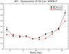Fig. A.1. Observed depolarization DP = pn, 20/pn, 6 between λ20.5 cm and λ6.2 cm in 1–kpc wide rings in the galaxy plane at 3′ resolution and predicted depolarization DP = DP20/DP6 by internal Faraday dispersion, using the observed variation in isotropic turbulent fields Bturb and thermal electron densities ⟨ne⟩. The statistical uncertainty in Bturb of ≃10% leads to an uncertainty of the predicted DP of ≃7%. The systematical uncertainty in ⟨ne⟩ of ≃20% causes a systematical uncertainty in DP of ≃14%.

All Tables

All Figures

	Fig. 1. Thermal intensity of M 31 at λ3.6 cm with $1\stackrel{\prime }{.}5$ resolution. The rms noise is ≃0.3 mJy/beam. Contour levels are at 0.5, 1, 2, and 3 mJy/beam. Bright background sources have been subtracted.
In the text

Fig. 2. Non-thermal intensity of M 31 at λ3.6 cm with $1\stackrel{\prime }{.}5$ resolution (corrected for AME) (top), at λ20.5 cm with $1\stackrel{\prime }{.}5$ resolution (middle), and at λ3.6 cm with $2\stackrel{\prime }{.}5$ resolution (corrected for AME) (bottom). The rms noise is ≃0.25 mJy/beam (top), ≃0.25 mJy/beam (middle), and ≃0.4 mJy/beam (bottom). Contour levels are at 0.75, 1.5, 2.25, 3.0, and 4.5 mJy/beam (top), 2.5, 5.0, 7.5, 10, 15, 20 mJy/beam (middle), and 1.25, 2.5, 3.75, and 7.5 mJy/beam (bottom). The half-power beam widths are indicated in the bottom left corner. Bright background sources and the unresolved central source of M 31 have been subtracted. At λ3.6 cm, large-scale emission is missing in the central region.

In the text

	Fig. 3. Radial variation in the intensities (in log scale) of the non-thermal (corrected for AME), thermal, and polarized emission at λ3.6 cm at $1\stackrel{\prime }{.}5$ resolution averaged in 0.5–kpc wide rings in the galaxy plane. In this and the following figures, the error bars show the 1-σ uncertainties.
In the text

Fig. 4. Top: Radial variation in the average spectral index, αn, of the non-thermal intensities at $1\stackrel{\prime }{.}5$ resolution between λ3.6 cm (corrected for AME) and λ20.5 cm in 0.5–kpc wide rings in the galaxy plane. Middle: Radial variations in the average spectral index, αn, of non-thermal intensities at 3′ resolution between λ3.6 cm (corrected for AME) and λ20.5 cm as well as between λ6.2 cm and λ20.5 cm in 1–kpc wide rings in the galaxy plane. Bottom: Radial variations in the average degrees of polarization, pn, of the non-thermal intensities at λ3.6 cm (corrected for AME) and at λ6.2 cm, both at 3′ resolution, at λ11.3 cm at 5′ resolution, and at λ20.5 cm at 3′ resolution.

In the text

Fig. 5. Maps of the strengths (in μG) of the total (top), isotropic turbulent (middle), and ordered magnetic fields in the sky plane (bottom) at $1\stackrel{\prime }{.}5$ resolution, computed from the total, unpolarized, and polarized non-thermal intensities at λ3.6 cm, assuming local equipartition between the energy densities of total magnetic fields and total CRs. Contour levels are at 7, 8, and 9 μG (total field and turbulent field), and 2.5, 3.5, and 4.5 μG (ordered field). Outside of the emission torus, synchrotron spectral indices are uncertain, so that no field strengths were computed.

In the text

	Fig. 6. Map of the strength of the total magnetic field (in μG), determined from the total non-thermal intensities at λ20.5 cm at $1\stackrel{\prime }{.}5$ resolution, assuming global (but not local) equipartition between the energy densities of total magnetic fields and total CRs. Contour levels are at 7, 8, and 9 μG. The colour scale is the same as that in Fig. 5 (top panel).
In the text

	Fig. 7. Variations in the strengths of the equipartition and non-equipartition total fields at $1\stackrel{\prime }{.}5$ resolution with azimuthal angle in the galaxy plane, counted from the north-eastern major axis in the sky plane (left side in Fig. 6), averaged in 10°–sectors of the radial ring 8–12 kpc.
In the text

	Fig. 8. Variation in RMs between λ3.6 cm and λ6.2 cm at 3′ resolution with azimuthal angle in the galaxy plane, averaged in 10°–sectors of the radial ring 8–12 kpc, and fitted by a sinusoidal line (in red).
In the text

	Fig. 9. Variations in the strengths of the (plane-of-sky) ordered, axisymmetric (ASS) regular, and anisotropic turbulent fields at $1\stackrel{\prime }{.}5$ resolution with azimuthal angle, measured in the galaxy plane in the radial ring 8–12 kpc, using the spiral pitch angle of the ASS field of −8° taken from the fit shown in Fig. 8.
In the text

	Fig. 10. ariations in the strengths of the plane-of-sky ordered, axisymmetric (ASS) regular, and anisotropic turbulent fields at $1\stackrel{\prime }{.}5$ resolution with azimuthal angle, measured in the galaxy plane in the radial ring 8–12 kpc, assuming a spiral pitch angle of the ASS field of −15°.
In the text

Fig. 11. Variations in the isotropic turbulent field strength, Bturb, (Fig. 5, middle panel) and the strength of the (plane-of-sky) anisotropic turbulent field Ban, ⊥ (taken from Fig. 10) at $1\stackrel{\prime }{.}5$ resolution with azimuthal angle in the galaxy plane in the radial ring 8–12 kpc. The uncertainties in Bturb reflect the dispersion of the values in the map of Bturb in each sector. The uncertainties in Ban, ⊥ come from the dispersion of the values in the map of Bord, ⊥ (Fig. 5, bottom panel) in each sector and the general uncertainty of Breg, ⊥ as determined in Sect. 4.6.

In the text

	Fig. 12. Average strengths (on a log scale) of the total, turbulent, and ordered fields at 3′ resolution in 1–kpc wide rings in the galaxy plane. The statistical uncertainties are assumed to be 10%. The systematical uncertainty of ≲20% (see Section 4.4) affects all values by the same amount and is not included.
In the text

Fig. 13. Average strengths (on a linear scale) of the turbulent and ordered fields (from Fig. 12) and of the regular field (Table 1) at 3′ resolution in 1–kpc wide rings in the galaxy plane. The uncertainties in Breg are estimated from the statistical uncertainties in RM and assuming a 5% uncertainty in ⟨ne⟩. The systematic uncertainties in Lth and fth of about 18% and 25%, respectively, affect all Breg values by the same amount and are not included.

In the text

Fig. A.1. Observed depolarization DP = pn, 20/pn, 6 between λ20.5 cm and λ6.2 cm in 1–kpc wide rings in the galaxy plane at 3′ resolution and predicted depolarization DP = DP20/DP6 by internal Faraday dispersion, using the observed variation in isotropic turbulent fields Bturb and thermal electron densities ⟨ne⟩. The statistical uncertainty in Bturb of ≃10% leads to an uncertainty of the predicted DP of ≃7%. The systematical uncertainty in ⟨ne⟩ of ≃20% causes a systematical uncertainty in DP of ≃14%.

In the text

References

- Arbutina, B., Urošević, D., Andjelić, M. M., Pavlović, M. Z., & Vukotić, B. 2012, ApJ, 746, 79 [Google Scholar]
- Arshakian, T. G., & Beck, R. 2011, MNRAS, 418, 2336 [NASA ADS] [CrossRef] [Google Scholar]
- Basu, A., & Roy, S. 2013, MNRAS, 433, 1675 [NASA ADS] [CrossRef] [Google Scholar]
- Basu, A., Roy, N., Beuther, H., et al. 2022, MNRAS, 517, 5063 [Google Scholar]
- Beck, R. 1982, A&A, 106, 121 [NASA ADS] [Google Scholar]
- Beck, R. 2007, A&A, 470, 539 [NASA ADS] [CrossRef] [EDP Sciences] [Google Scholar]
- Beck, R. 2015, A&A, 578, A93 [NASA ADS] [CrossRef] [EDP Sciences] [Google Scholar]
- Beck, R., & Krause, M. 2005, Astron. Nachr., 326, 414 [Google Scholar]
- Beck, R., Loiseau, N., Hummel, E., et al. 1989, A&A, 222, 58 [NASA ADS] [Google Scholar]
- Beck, R., Brandenburg, A., Moss, D., Shukurov, A., & Sokoloff, D. 1996, ARA&A, 34, 155 [NASA ADS] [CrossRef] [Google Scholar]
- Beck, R., Berkhuijsen, E. M., & Hoernes, P. 1998, A&AS, 129, 329 [NASA ADS] [CrossRef] [EDP Sciences] [Google Scholar]
- Beck, R., Shukurov, A., Sokoloff, D., & Wielebinski, R. 2003, A&A, 411, 99 [NASA ADS] [CrossRef] [EDP Sciences] [Google Scholar]
- Beck, R., Chamandy, L., Elson, E., & Blackman, E. G. 2019, Galaxies, 8, 4 [NASA ADS] [CrossRef] [Google Scholar]
- Beck, R., Berkhuijsen, E. M., Gießübel, R., & Mulcahy, D. D. 2020, A&A, 633, A5 [EDP Sciences] [Google Scholar]
- Bell, A. R. 1978, MNRAS, 182, 443 [Google Scholar]
- Berkhuijsen, E. M., Beck, R., & Hoernes, P. 2003, A&A, 398, 937 [NASA ADS] [CrossRef] [EDP Sciences] [Google Scholar]
- Berkhuijsen, E. M., Mitra, D., & Müller, P. 2006, Astron. Nachr., 327, 82 [NASA ADS] [CrossRef] [Google Scholar]
- Berkhuijsen, E. M., Beck, R., & Tabatabaei, F. S. 2013, MNRAS, 435, 1598 [Google Scholar]
- Berkhuijsen, E. M., Urbanik, M., Beck, R., & Han, J. L. 2016, A&A, 588, A114 [NASA ADS] [CrossRef] [EDP Sciences] [Google Scholar]
- Bhat, P., Subramanian, K., & Brandenburg, A. 2016, MNRAS, 461, 240 [Google Scholar]
- Boulares, A., & Cox, D. P. 1990, ApJ, 365, 544 [NASA ADS] [CrossRef] [Google Scholar]
- Brandenburg, A., & Ntormousi, E. 2023, ARA&A, 61, 561 [CrossRef] [Google Scholar]
- Brandenburg, A., & Subramanian, K. 2005, Phys. Rep., 417, 1 [NASA ADS] [CrossRef] [Google Scholar]
- Brandt, P. C., Provornikova, E., Bale, S. D., et al. 2023, Space Sci. Rev., 219, 18 [NASA ADS] [CrossRef] [Google Scholar]
- Braun, R. 1991, ApJ, 372, 54 [NASA ADS] [CrossRef] [Google Scholar]
- Braun, R., Thilker, D. A., Walterbos, R. A. M., & Corbelli, E. 2009, ApJ, 695, 937 [Google Scholar]
- Brinks, E., & Shane, W. W. 1984, A&AS, 55, 179 [NASA ADS] [Google Scholar]
- Caldú-Primo, A., Schruba, A., Walter, F., et al. 2013, AJ, 146, 150 [CrossRef] [Google Scholar]
- Chamandy, L. 2016, MNRAS, 462, 4402 [NASA ADS] [CrossRef] [Google Scholar]
- Chemin, L., Carignan, C., & Foster, T. 2009, ApJ, 705, 1395 [NASA ADS] [CrossRef] [Google Scholar]
- Chuvilgin, L. G., & Ptuskin, V. S. 1993, A&A, 279, 278 [NASA ADS] [Google Scholar]
- Dacunha, T., Martin-Alvarez, S., Clark, S. E., & Lopez-Rodriguez, E. 2025, ApJ, 980, 197 [Google Scholar]
- Devereux, N. A., Price, R., Wells, L. A., & Duric, N. 1994, AJ, 108, 1667 [Google Scholar]
- Dickey, J. M., & Brinks, E. 1988, MNRAS, 233, 781 [Google Scholar]
- Dickinson, C., Davies, R. D., & Davis, R. J. 2003, MNRAS, 341, 369 [NASA ADS] [CrossRef] [Google Scholar]
- Ehle, M., & Beck, R. 1993, A&A, 273, 45 [NASA ADS] [Google Scholar]
- Evirgen, C. C., Gent, F. A., Shukurov, A., Fletcher, A., & Bushby, P. J. 2019, MNRAS, 488, 5065 [Google Scholar]
- Fatigoni, S., Radiconi, F., Battistelli, E. S., et al. 2021, A&A, 651, A98 [NASA ADS] [CrossRef] [EDP Sciences] [Google Scholar]
- Federrath, C., Schober, J., Bovino, S., & Schleicher, D. R. G. 2014, ApJ, 797, L19 [NASA ADS] [CrossRef] [Google Scholar]
- Fernández-Torreiro, M., Génova-Santos, R. T., Rubiño-Martín, J. A., et al. 2024, MNRAS, 527, 11945 [Google Scholar]
- Ferrière, K. M. 2001, Rev. Mod. Phys., 73, 1031 [NASA ADS] [CrossRef] [Google Scholar]
- Ferrière, K. 2020, Plasma Phys. Contr. Fus., 62, 014014 [Google Scholar]
- Fletcher, A., Berkhuijsen, E. M., Beck, R., & Shukurov, A. 2004, A&A, 414, 53 [NASA ADS] [CrossRef] [EDP Sciences] [Google Scholar]
- Fletcher, A., Beck, R., Shukurov, A., Berkhuijsen, E. M., & Horellou, C. 2011, MNRAS, 412, 2396 [CrossRef] [Google Scholar]
- Fritz, J., Gentile, G., Smith, M. W. L., et al. 2012, A&A, 546, A34 [NASA ADS] [CrossRef] [EDP Sciences] [Google Scholar]
- Gaensler, B. M., Madsen, G. J., Chatterjee, S., & Mao, S. A. 2008, PASA, 25, 184 [NASA ADS] [CrossRef] [Google Scholar]
- Gent, F. A., Mac Low, M.-M., Korpi-Lagg, M. J., & Singh, N. K. 2023, ApJ, 943, 176 [NASA ADS] [CrossRef] [Google Scholar]
- Gent, F. A., Mac Low, M.-M., & Korpi-Lagg, M. J. 2024, ApJ, 961, 7 [NASA ADS] [CrossRef] [Google Scholar]
- Gießübel, R., & Beck, R. 2014, A&A, 571, A61 [NASA ADS] [CrossRef] [EDP Sciences] [Google Scholar]
- Gordon, K. D., Bailin, J., Engelbracht, C. W., et al. 2006, ApJ, 638, L87 [Google Scholar]
- Han, J. L., Beck, R., & Berkhuijsen, E. M. 1998, A&A, 335, 1117 [NASA ADS] [Google Scholar]
- Han, J. L., Ferriere, K., & Manchester, R. N. 2004, ApJ, 610, 820 [Google Scholar]
- Heesen, V., Buie, E. I., Huff, C. J., et al. 2019, A&A, 622, A8 [NASA ADS] [CrossRef] [EDP Sciences] [Google Scholar]
- Heesen, V., Klocke, T. L., Brüggen, M., et al. 2023, A&A, 669, A8 [NASA ADS] [CrossRef] [EDP Sciences] [Google Scholar]
- Hollins, J. F., Sarson, G. R., Shukurov, A., Fletcher, A., & Gent, F. A. 2017, ApJ, 850, 4 [NASA ADS] [CrossRef] [Google Scholar]
- Krause, M., Hummel, E., & Beck, R. 1989, A&A, 217, 4 [NASA ADS] [Google Scholar]
- Krause, M., Irwin, J., Wiegert, T., et al. 2018, A&A, 611, A72 [NASA ADS] [CrossRef] [EDP Sciences] [Google Scholar]
- Krumholz, M. R., & Federrath, C. 2019, Front. Astron. Space Sci., 6, 7 [NASA ADS] [CrossRef] [Google Scholar]
- Moskalenko, I. V., Strong, A. W., Ormes, J. F., & Potgieter, M. S. 2002, ApJ, 565, 280 [NASA ADS] [CrossRef] [Google Scholar]
- Mulcahy, D. D., Horneffer, A., Beck, R., et al. 2014, A&A, 568, A74 [NASA ADS] [CrossRef] [EDP Sciences] [Google Scholar]
- Mulcahy, D. D., Fletcher, A., Beck, R., Mitra, D., & Scaife, A. M. M. 2016, A&A, 592, A123 [NASA ADS] [CrossRef] [EDP Sciences] [Google Scholar]
- Nasirzadeh, M. R., Tabatabaei, F. S., Beck, R., et al. 2024, A&A, 691, A199 [NASA ADS] [CrossRef] [EDP Sciences] [Google Scholar]
- Nieten, C., Neininger, N., Guélin, M., et al. 2006, A&A, 453, 459 [CrossRef] [EDP Sciences] [Google Scholar]
- Pakmor, R., Bieri, R., van de Voort, F., et al. 2024, MNRAS, 528, 2308 [NASA ADS] [CrossRef] [Google Scholar]
- Paul, I., Vasanth Kashyap, R., Ghosh, T., et al. 2025, MNRAS, submitted [arXiv:2506.13954] [Google Scholar]
- Pillepich, A., Sotillo-Ramos, D., Ramesh, R., et al. 2024, MNRAS, 535, 1721 [NASA ADS] [CrossRef] [Google Scholar]
- Ponnada, S. B., Panopoulou, G. V., Butsky, I. S., et al. 2022, MNRAS, 516, 4417 [NASA ADS] [CrossRef] [Google Scholar]
- Ponnada, S. B., Panopoulou, G. V., Butsky, I. S., et al. 2024, MNRAS, 527, 11707 [Google Scholar]
- Rahmani, S., Lianou, S., & Barmby, P. 2016, MNRAS, 456, 4128 [NASA ADS] [CrossRef] [Google Scholar]
- Rieder, M., & Teyssier, R. 2017, MNRAS, 471, 2674 [NASA ADS] [CrossRef] [Google Scholar]
- Rodrigues, L. F. S., Chamandy, L., Shukurov, A., Baugh, C. M., & Taylor, A. R. 2019, MNRAS, 483, 2424 [NASA ADS] [CrossRef] [Google Scholar]
- Ruszkowski, M., & Pfrommer, C. 2023, A&ARv, 31, 4 [NASA ADS] [CrossRef] [Google Scholar]
- Seta, A., & Beck, R. 2019, Galaxies, 7, 45 [NASA ADS] [CrossRef] [Google Scholar]
- Seta, A., & Federrath, C. 2020, MNRAS, 499, 2076 [NASA ADS] [CrossRef] [Google Scholar]
- Seta, A., & Federrath, C. 2022, MNRAS, 514, 957 [NASA ADS] [CrossRef] [Google Scholar]
- Seta, A., Shukurov, A., Wood, T. S., Bushby, P. J., & Snodin, A. P. 2018, MNRAS, 473, 4544 [NASA ADS] [CrossRef] [Google Scholar]
- Shukurov, A. M., & Subramanian, K. 2021, Astrophysical Magnetic Fields: From Galaxies to the Early Universe (Cambridge: Cambridge University Press) [Google Scholar]
- Sofue, Y., & Beck, R. 1987, PASJ, 39, 541 [NASA ADS] [Google Scholar]
- Sokoloff, D. D., Bykov, A. A., Shukurov, A., et al. 1998, MNRAS, 299, 189 [Google Scholar]
- Stepanov, R., Shukurov, A., Fletcher, A., et al. 2014, MNRAS, 437, 2201 [Google Scholar]
- Strong, A. W. 2007, Ap&SS, 309, 35 [Google Scholar]
- Tabatabaei, F. S., & Berkhuijsen, E. M. 2010, A&A, 517, A77 [NASA ADS] [CrossRef] [EDP Sciences] [Google Scholar]
- Tabatabaei, F. S., Krause, M., Fletcher, A., & Beck, R. 2008, A&A, 490, 1005 [NASA ADS] [CrossRef] [EDP Sciences] [Google Scholar]
- Tabatabaei, F. S., Schinnerer, E., Murphy, E. J., et al. 2013a, A&A, 552, A19 [NASA ADS] [CrossRef] [EDP Sciences] [Google Scholar]
- Tabatabaei, F. S., Berkhuijsen, E. M., Frick, P., Beck, R., & Schinnerer, E. 2013b, A&A, 557, A129 [NASA ADS] [CrossRef] [EDP Sciences] [Google Scholar]
- Tabatabaei, F. S., Schinnerer, E., Krause, M., et al. 2017, ApJ, 836, 185 [Google Scholar]
- Tabatabaei, F. S., Minguez, P., Prieto, M. A., & Fernández-Ontiveros, J. A. 2018, Nat. Astron., 2, 83 [Google Scholar]
- Tharakkal, D., Shukurov, A., Gent, F. A., Sarson, G. R., & Snodin, A. 2023a, MNRAS, 525, 2972 [CrossRef] [Google Scholar]
- Tharakkal, D., Snodin, A. P., Sarson, G. R., & Shukurov, A. 2023b, Phys. Rev. E, 107, 065206 [Google Scholar]
- Tribble, P. C. 1991, MNRAS, 250, 726 [NASA ADS] [CrossRef] [Google Scholar]
- Vollmer, B., Soida, M., Beck, R., & Powalka, M. 2020, A&A, 633, A144 [NASA ADS] [CrossRef] [EDP Sciences] [Google Scholar]
- Walterbos, R. A. M., & Braun, R. 1994, ApJ, 431, 156 [NASA ADS] [CrossRef] [Google Scholar]
- Williams, A. L., Heald, G., Wilcots, E. M., & Zweibel, E. G. 2024, ApJ, 961, 238 [Google Scholar]
- Yan, H., & Lazarian, A. 2004, ApJ, 614, 757 [NASA ADS] [CrossRef] [Google Scholar]
- Zweibel, E. G. 2013, Phys. Plasmas, 20, 055501 [NASA ADS] [CrossRef] [Google Scholar]
- Zychowicz, A. A., & Chyży, K. T. 2025, ApJS, 276, 41 [Google Scholar]