| Issue |
A&A
Volume 700, August 2025
|
|
|---|---|---|
| Article Number | A106 | |
| Number of page(s) | 13 | |
| Section | Planets, planetary systems, and small bodies | |
| DOI | https://doi.org/10.1051/0004-6361/202555457 | |
| Published online | 08 August 2025 | |
A complete census of planet-hosting binaries
1
LIRA, Observatoire de Paris, Université PSL,
5 Place Jules Janssen,
92195
Meudon,
France
2
Sapienza Università di Roma,
Piazzale Aldo Moro 5,
00185
Rome,
Italy
★ Corresponding author.
Received:
9
May
2025
Accepted:
23
June
2025
Abstract
Aims. Estimating the effect that binarity can have on planet formation is of crucial importance, as almost half of field stars reside in multiple systems. One effective way to assess this effect is to get an accurate picture of the population of planet-hosting binaries and compare the characteristics to those of field star binaries.
Methods. We have constructed an extensive database through intensive literature exploration to achieve a complete census of all planet-hosting binaries known to date. Despite the heterogeneous character of the different surveys this database is built on and the biases and selection effects that unavoidably affect any sample of planet-hosting binaries, we looked for statistically significant trends and correlations within our sample.
Results. Our database provides the characteristics (orbit or projected separation, stellar masses, distance, dynamical stability) for 759 systems (among which 31 are circumbinaries), representing an increase by a factor of nine with respect to the previous complete census of planet-hosting binaries. Of the 728 S-type systems, 651 are binaries, 73 are triples, and 4 are quadruples. The raw distribution of planet-hosting binary separations peaks around 500 au instead of 50 au for field binaries. By analysing the distribution of on-sky angular separations as a function of distance (db) to the systems, we argue that the observed deficit of planet-hosting close-in binaries cannot be explained solely by observational biases. Likewise, by exploring how multiplicity fractions among planet hosts vary with db, we suggest that the subsample of known planet-hosting binaries at <500 pc is not bias dominated (but also not bias-free). In this <500 pc domain, the multiplicity fraction of planet-hosting stars is ~22.5%, which is approximately half of the value for field stars, and the deficit of binaries extends to separations of ~500 au, giving an approximate estimate of the detrimental effect binarity has on planet formation.
Key words: planets and satellites: formation / binaries: general
© The Authors 2025
 Open Access article, published by EDP Sciences, under the terms of the Creative Commons Attribution License (https://creativecommons.org/licenses/by/4.0), which permits unrestricted use, distribution, and reproduction in any medium, provided the original work is properly cited.
This article is published in open access under the Subscribe to Open model. This email address is being protected from spambots. You need JavaScript enabled to view it. to support open access publication.
1 Introduction
The multiplicity fraction of field stars in the solar neighbourhood is almost 50% (Raghavan et al. 2010). Given that binarity should thus be a relatively common environment, the study of exoplanets in the context of binaries is of crucial importance. Theoretical studies have shown that some stages of the planet-formation process can be significantly affected by the presence of a stellar companion. Binary perturbations could, for example, truncate primordial protoplanetary discs (Savonije et al. 1994), which on the one hand could deplete them of too much mass to be able to form planets and, on the other hand, shorten their lifetime below what is required for core accretion (e.g. Müller & Kley 2012). A stellar companion could also affect the planetesimal-accretion stage by increasing impact velocities to values that could prevent, or at least slow, growth by mutual accretion (Thebault et al. 2006; Thebault 2011), even though disc self-gravity could counteract, to some extent, this detrimental effect (Silsbee & Rafikov 2021). (For a review on planet formation in the context of binaries, see Thebault & Haghighipour 2015 and Marzari & Thebault 2019.)
Regardless of these theoretical considerations, another way to assess the influence of binarity on planet formation is to consider the population of observed exoplanet systems and look for potential differences between systems around single stars and systems in binaries. The most straightforward procedure would be to compare the occurrence rate of planets in single systems to that of planets in binaries. Such an analysis is, however, very difficult to perform in practice, as it requires precise information about the samples of binaries that have been explored in every planet-searching survey. One of the few attempts at comparing planet occurrence rates in single systems and binaries was carried out by Hirsch et al. (2021), who considered a volume-limited (<25pc) and unbiased sample of single and multiple stellar systems for which a relative velocity (RV) search for giant (>0.1 MJup) exoplanets was performed. They concluded that giant planet occurrence is ~12% in binaries and ~18% for single systems. However, the occurrence rate in wide >100 au binaries seemed to be compatible with that in singles. It is only occurrences in close binaries that are significantly lower (~4%), thus supporting the argument of a detrimental effect of close binaries on planet formation. These results, however, should be considered with caution given the limited size of the binaries-with-planets sample they are based on (eight systems in total and only one closer than 100 au).
In practice, the most common way to investigate the effect binarity can have on planetary systems is to consider the problem the other way around, that is, to look for differences in the binarity fraction between exoplanet hosts and field stars. Early on, it was noticed that the multiplicity fraction among planet hosts is relatively low: 23% in Raghavan et al. (2006), 17% in Mugrauer & Neuhäuser (2009), or 12% in Roell et al. (2012), as compared to the derived value of 46% for FGK field stars in the solar vicinity (Raghavan et al. 2010). It was quickly understood that these low values were, at least partially, due to strong observational biases. For the RV method, companion stars too close to the primary can indeed pollute the signal so that binaries with separations ≲1–2″ (and even sometimes up to 5″) were initially excluded from most surveys (Eggenberger et al. 2007; Hirsch et al. 2021). The transit method, in principle, does not suffer from such strong adverse selection effects, even though it is not fully bias-free – the additional flux of the companion star decreases the transit depth and could make it sink below the (S/N) threshold for identifying, for example, Kepler objects of interest (KOIs) or Tess objects of interest (TOIs) (Wang et al. 2015; Ziegler et al. 2020). In addition, stars targeted by transit surveys, in particular the ones performed with the Kepler telescope, are generally relatively distant and had often not been vetted for binarity so that, at least initially, a significant fraction could have been wrongly mislabelled as singles. To alleviate this issue, large surveys have been undertaken using adaptive optics (AO) or ‘lucky imaging’ to search for stellar companions around KOIs and TOIs (e.g. Kraus et al. 2016; Furlan et al. 2017; Ziegler et al. 2020). More recently this search for companions has been performed by mining the Gaia DR2 and DR3 catalogues to look for common parallaxes and proper motions (Mugrauer & Michel 2020, 2021; Fontanive & Bardalez Gagliuffi 2021; González-Payo et al. 2024; Michel & Mugrauer 2024).
Interestingly, these surveys reach conclusions that sometimes contradict each other, even when considering the same category of planet-hosts. For the subsample of KOIs, for example, Horch et al. (2014) conclude that the multiplicity fraction is comparable to that of field stars, while Kraus et al. (2016) find a strong deficit of planet-hosting binaries with separations ≲50–100 au, and Wang et al. (2014) conclude that the binary deficit even extends to separations of 1500au. We note, however, that the most recent surveys considering large samples of planet hosts all find raw global multiplicity rates of around 20%, i.e. about one half of that for field stars: 23.2% in Fontanive & Bardalez Gagliuffi (2021), 19% for Michel & Mugrauer (2024), or 21.7% in González-Payo et al. (2024). However, a debate remains as to whether these low values are uniquely due to selection effects and the incompleteness of close (typically ≲50 au) binary censuses for distant targets (such as KOIs) or if this ~50% deficit of planet-hosting binaries is real and physical. González-Payo et al. (2024) attributes all the deficit to biases and adverse selection effects, while Fontanive & Bardalez Gagliuffi (2021) and Michel & Mugrauer (2024) remain more cautious.
In this work, we present a census of all known planet-hosting multiples to date, compiling 759 systems (among which 31 are circumbinaries), which corresponds to a factor of nine increase with respect to the last complete census of Martin (2018). Our goal is twofold. First, we seek to provide a complete database to the community that will be regularly updated in an online-accessible file. Second, our aim is to use the unprecedented size of our sample (allowing us to explore correlations, such as multiplicity fraction as a function of distance, which has not been explored before) to derive statistically robust results about the characteristics of planet-hosting binaries despite the unavoidable observational biases affecting our sample.
The paper is organised as follows: in Sect. 2 we describe the procedure by which the database was built and the information it provides. Sect. 3 presents the complete database and an exploration of the statistical correlations between crucial parameters (e.g. separation, system distance, multiplicity fractions). The robustness and reliability of our results is discussed in Sect. 4. In Sect. 5, we summarise our results and main conclusions.
2 Building the database
2.1 Definition and boundaries
Our database compiles all the confirmed stellar companions of confirmed (i.e. not candidate) planet hosts. We adopted the conservative policy of excluding brown dwarfs and only considering hosts of ‘planets’ with a mass (or a minimum mass) ≤13 MJup, the limit for deuterium burning (Morley et al. 2024). Likewise, we only considered ‘stellar’ companions of mass M ≥ 75MJup, thus again excluding brown dwarfs (Chabrier et al. 2023). This allowed us to have a well-defined separation between planetary and stellar companions. Our main database concerns systems with an ‘S-type’ configuration, where the planet(s) orbits(-) one component of the binary, but we also compiled a separate database for circumbinary cases (‘P-type’ orbits), which is presented in Sect. 3.6. The following information is provided for all systems: name(s), masses of the stellar components, orbital parameters of the binary (ab, eb, and, for some rare cases, ib), distance to the system, method of planet detection, number of known planets (nPl), mass (mPl), and orbit (aPl and epl) of the outermost planet (i.e. the one most affected by the stellar companion’s perturbations).
2.2 Orbital stability
For each system, we also estimated the outer limit for orbital stability, acrit, which is the maximum radial distance to the planet-host star for which orbits are stable despite the companion’s perturbations. We derived acrit using the widely used empirical formula from Holman & Wiegert (1999). We note that for most systems (especially those of separation ≥50 au), only the projected separation between the stars is known, while the actual orbit of the binary remains unconstrained. In this case the database only provides the projected separation (ρb). To derive acrit for these non-constrained orbits, we considered a ‘statistical’ semi-major axis using the average relation log(ab) = log(ρb) + 0.13 derived by Duquennoy & Mayor (1991) for randomly distributed orbits and an eccentricity <eb> corresponding to the average value of 0.45 derived by Raghavan et al. (2010) for field binaries near the sun. For these cases, the estimated stability limit thus only gives a first-order estimate and should be taken with caution.
2.3 Higher-order multiples
Some of the ‘binaries’ listed in the database are in fact higher-order multiple systems, mostly triple or even quadruple stellar systems. However, most of these systems can be approximated as binaries from a dynamical point of view. The vast majority of them are indeed highly hierarchical and fall into two main categories:
Systems where the companion star is itself a tight or spectroscopic binary. In this A-(BC) case, the dynamical behaviour of the circumprimary planetary system is very close to the case with one ‘virtual’ stellar companion of mass MB + MC.
Systems where the third star is much more distant (typically more than ten times) from the central primary than the secondary. In this case, the third star does not significantly impact the dynamical evolution of the planetary system, and its influence can be neglected in a first approximation.
Therefore, for the sake of clarity and simplicity and in order to not artificially reduce the size of the sample on which we derived the general trends (see Sect. 3), the hierarchical triples are presented as binaries in the main database by means of a ‘virtual’ merged BC companion or by neglecting the too distant C component. The dynamical stability outer limit (acrit) of the planet was then computed with these simplified approximations. These hierarchical triples are indicated with an asterisk (*) placed at the end of the system’s name. The exact description of these systems is given in the ‘Notes and references on individual systems’ Table C.1.
Complete database of planet-hosting ‘S-type’ binaries, sorted by increasing binary separation.
2.4 Sources
Our database is mostly based on a deep and thorough investigation of the literature. Our main sources are surveys that searched for stellar companions to planet-hosting stars. As mentioned in Sect. 1, these surveys are mainly of two different types: high-precision imaging (AO, speckle) or mining of the Gaia DR2 and DR3 database. We note that we only compiled confirmed stellar companions, so the companions identified in the imaging surveys were only considered if there was an additional analysis that allowed to distinguish between a physical bound companion and a background object. This additional vetting was generally either astrometric (looking for common parallaxes and proper motions) or photometric (multi-band analysis to check if colors are consistent with a main-sequence companion rather than a background object). We made an exception to this rule for a handful of companions detected in imagery for which the statistical chances of being a background object were less than 1% (Ziegler et al. 2020). We note that we also only considered systems with confirmed (i.e. not candidate) planets, thus eliminating a significant fraction of stellar companions found around KOIs or TOIs that have not yet been confirmed as planets. It is thus necessary to regularly go back to the source surveys, as some planets that were candidates at the time of the survey have since been confirmed.
In some cases, the binarity of the system is not assessed in a later survey but directly in the planet-discovery study. Notably, this is the case for most systems detected by microlensing (e.g. Gould et al. 2014; Poleski et al. 2014), but it also occurs for a non-negligible number of RV or transit detections (e.g. Howard et al. 2010; Buchhave et al. 2011; Beatty et al. 2012). Finally, there is a small (but non-negligible) fraction of our sample for which the binarity has been long known and taken from catalogues, such as the Washington Double Star Catalog (WDS, Mason et al. 2001).
There is a significant fraction of stellar companions that have been identified in several separate surveys. In these cases, we tried to give credit (see the “Notes and references on individual systems” Table C.1) to the earliest work that assessed the binarity. With respect to the binary characteristics (e.g. stellar mass, distance, projected separation), we considered the constraints obtained from the most recent study. Table A.1 gives a non-exhaustive list of the main sources we used.
3 Results
Table 1 presents our complete database, which compiles 728 ‘S-type’ planet-hosting multiples. This is more than twice the size of the largest samples considered in earlier studies (348 systems in Michel & Mugrauer 2024) and almost ten times the size of the last published full census of planets in binaries (Martin 2018). This database will be regularly updated and will be available to the community in an online version1 hosted on the website of the Encyclopaedia of Exoplanetary Systems (Schneider et al. 2011).
3.1 Separation distribution
We present in Fig. 1 a histogram of the distribution of the binary semi-major axis (ab) in our planet-hosting binaries sample. This distribution peaks at around 500 au, which corresponds to a pronounced deficit of close-in companions when compared to the canonical distribution of Raghavan et al. (2010). Using a bootstrap resampling procedure on the log(ab) distribution of our planet-hosting binaries sample, we obtained ![Mathematical equation: $\[< ~a_{b}>=737_{-88}^{+133}\]$](/articles/aa/full_html/2025/08/aa55457-25/aa55457-25-eq1.png) au at the 3σ confidence level, confirming that this distribution is statistically different from that of field binaries, which peaks at 45 au2. This deficit of tight planet-hosting binaries is a well known feature, and it was identified in earlier studies for smaller binary samples (e.g. Kraus et al. 2016). As mentioned in Sect. 1, the main questions are to what extent this depletion is due to observational biases or adverse selection effects and to what extent is it a real physical feature. Answering these questions might appear less straightforward for the present sample given the all-encompassing nature of our census and the heterogeneity of the sources it is built on compared to more limited and homogeneous surveys (such as volume-limited studies targeting only KOIs or TOIs). The size of our sample does, however, allow us to explore parameters that can help put constraints on the level of bias (or lack thereof) affecting our census.
au at the 3σ confidence level, confirming that this distribution is statistically different from that of field binaries, which peaks at 45 au2. This deficit of tight planet-hosting binaries is a well known feature, and it was identified in earlier studies for smaller binary samples (e.g. Kraus et al. 2016). As mentioned in Sect. 1, the main questions are to what extent this depletion is due to observational biases or adverse selection effects and to what extent is it a real physical feature. Answering these questions might appear less straightforward for the present sample given the all-encompassing nature of our census and the heterogeneity of the sources it is built on compared to more limited and homogeneous surveys (such as volume-limited studies targeting only KOIs or TOIs). The size of our sample does, however, allow us to explore parameters that can help put constraints on the level of bias (or lack thereof) affecting our census.
A compelling indication that the lack of planet-hosting tight binaries cannot be entirely due to observational biases follows from plotting binary projected angular separations (θb) as a function of distance (db) to the system (Fig. 2). Since the main adverse selection effects (see Sect. 1) against binaries are, to a first order, inversely proportional to the angular separation between stellar components, we would indeed expect the lower envelope of the (θb,db) distribution to be horizontal in a bias-dominated sample. This is clearly not what is observed in Fig. 2, which shows that, on the contrary, the lower envelope of the (θb,db) distribution follows an inclined ρb~cst line (see Sect. 4.1 for more discussion on this issue).
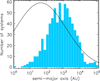 |
Fig. 1 Histogram of planet-hosting binary semi-major axis for the complete sample. When only the projected separation (ρb) is known, a ‘statistical’ semi-major axis is considered following the relation derived by Duquennoy & Mayor (1991) for randomly distributed orbits (see text for details). The black line corresponds to the normalised distribution for field stars derived by Raghavan et al. (2010). |
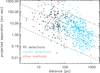 |
Fig. 2 On-sky projected angular separation (θb) between binary components as a function of distance (db) to the system. The four black lines correspond (from bottom to top) to physical separations of 10, 100, 1000, and 10 000 au. We note that Proxima Centauri has been left out of this graph in order not to ‘squeeze’ the graph’s Y-axis. |
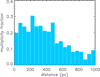 |
Fig. 3 Multiplicity fraction of confirmed planet hosts as a function of distance to the system. |
3.2 Multiplicity fraction
To compute the multiplicity fractions amongst the planet host stars, we took the up-to-date population of planet-hosting systems in the Encyclopaedia of Exoplanetary Systems3 as a reference. As of May 2025, the total number of systems hosting at least one ≤13 MJup planet is 4504. This gives a raw multiplicity fraction (fM) for the whole sample that is equal to 728/4504=0.161. This is slightly lower than the ~20% found in recent surveys (see Sect. 1) and much lower than the 0.46 fraction derived by Raghavan et al. (2010) for field stars.
As with the separation distribution, the issue to assess here is to what extent this fM value is affected by observation biases and selection effects. Plotting how this parameter varies with distance can here again provide some important clues. As can be seen in Fig. 3, the multiplicity fraction is indeed almost constant in the db < 500 pc domain, which is not what would be expected for a sample dominated by biases, for which fM should decrease with increasing distance. This is here again because the main adverse biases affecting our sample become more pronounced with a decreasing on-sky angular separation between the binary components, thus leading to lower fM values at larger db. This expected decrease of fM values is in fact observed, but only beyond ~500 pc4, indicating that it is only in this distance domain that the sample becomes bias dominated. We discuss these issues in more detail in Sect. 4.2, but we assume from here on that the region at db < 500 pc provides global statistics that are, to a first order, reliable. For these db < 500 pc systems, the global multiplicity fraction increases to fM = 22.5% (Table 2), which is comparable to the 23.2% in Fontanive & Bardalez Gagliuffi (2021), 19% for Michel & Mugrauer (2024), or 21.7% in González-Payo et al. (2024). We argue that this value is probably close to the real unbiased value for planet-bearing binaries (see discussion in Sect. 4).
Multiplicity fraction (fM) for the whole population of exoplanet hosts as well as a function of stellar type (for the planet-bearing star).
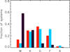 |
Fig. 4 Fraction of planet-hosting primaries (blue) and stellar companions (deep purple) in our database as a function of stellar type. The red histogram corresponds to the distribution for planet-hosting single stars (taken from the Encyclopaedia of Exoplanetary Systems). |
3.3 Stellar types
The vast majority of the planet-hosting primaries consist of K-G-F stellar types (Fig. 4), which make up more than 90% of our sample. We note that this stellar type distribution of primaries is a close match to that for planet-hosting single stars, the only difference being a slight deficit of M stars and a slight excess of F types. In contrast, the population of companion stars is completely dominated by low-mass M stars, which account for 58% of this subsample. These results agree relatively well with those obtained by Fontanive & Bardalez Gagliuffi (2021) on a more limited sample.
When looking at the multiplicity fraction for each stellar type (Table 2), we observed that it progressively increases from M to F stars, which does qualitatively agree with the trend observed among field binaries (Raghavan et al. 2010). However, the differences between the different stellar types are more pronounced than for field binaries. As an example, fM(Fstars)/ fM(Mstars) ~ 3 for planet hosts, whereas this ratio is only equal to ~1.6 for field stars. This could indicate that the detrimental effect of binarity on planet formation increases with decreasing stellar mass.
Planet semi-major axis (aPl) and projected separations (ρAB and ρAC) of the stellar companions for the three non-hierarchical planetbearing triples.
3.4 Triples and higher-order multiples
3.4.1 Occurrence rate
Our census lists 77 higher-order multiples (73 triples and 4 quadruples), corresponding to 10.6% (or 12.4% if only considering systems at <500 pc) of our total sample of 728 planet-hosting S-type multiples. This value is close to the one obtained by Michel & Mugrauer (2024), 12%, but it is significantly lower than the 19.5% for field stars found by Raghavan et al. (2010). As pointed out by González-Payo et al. (2024), such lower values might be due to the fact that if planet-hosting primaries have been investigated by companion-search surveys, their identified companions (especially wide ones) have not been investigated as thoroughly, so a significant fraction of wide planet-hosting binaries might in fact be triples (where the companion star itself is a yet undetected binary).
3.4.2 Non-hierarchical triples
As mentioned in Sect. 2.3, the vast majority of the triples in our subsample are hierarchical, with the ratio between the separations of the two different binary pairs being higher than ten. However, we identified three rare non-hierarchical triples (see Table 3) for which the dynamical role of the third component cannot in principle be neglected. We note, however, that for all three systems, only the projected separations (ρAB and ρAC) of the stellar companions are known, and the inclination between the A-B and B-C orbital planes is not constrained. Thus, we could not rule out that these three cases are in fact hierarchical because the third component is in reality much farther away from the primary than ρAC.
3.4.3 Planets on both S-type and P-type orbits
In four systems (HD 155555, BX Tri, Kepler-64, and KIC 7177553), the central planet-hosting star is itself a very tight binary (ab ≤ 0.2 au). In these cases, the planet is actually on both an S-type and a P-type orbit. Since all four systems are highly hierarchical, we list them in our main database as S-types, for which we assume a ‘virtual’ primary by adding the masses of the two inner components, and also in our separate database of circumbinary systems (see Sect. 3.6), in which we neglect the influence of the third outer stellar component.
3.5 Architecture and stability
Figure 5 presents the dynamical architecture for the 100 tightest planet-hosting binaries, with projected separation up to ~75 au. For each system we plot (as a vertical bar) the location of the outer planetary orbit stability limit (acrit) given by the empirical formula of Holman & Wiegert (1999) as a function of ab, eb, and μb (mass ratio between the binary components). For the cases where ab and eb are unconstrained and only the projected separation (ρb) is known, we considered three different (ab, eb) configurations (and thus three different acrit): one reference case assuming the ‘statistical orbit’ log(ab) = log(ρb) + 0.13 and eb = 0.45 (see Sect. 2.2); one ‘low eb’ case with ab = ρb and eb = 0; and one ‘high-eb’ case with ab = ρb and eb = 0.7. It can be seen that for almost all systems, planets are located in the dynamically ‘safe’ ap ≤ acrit region around the planet-hosting star. There are only three systems with constrained binary orbits for which ap lies beyond acrit: HD 59686, Kepler-1505, and TOI-4633. In all three cases it is the very high value of eb − 0.91 for TOI-4633, 0.97 for Kepler-1505 (but with a very large uncertainty on eb, see Lester et al. 2023) and 0.73 for HD 59686 – that is responsible for this dynamically ‘unsafe’ situation. Trifonov et al. (2018) thoroughly investigated HD 59686’s dynamics and found that there is nevertheless a relatively large parameter space for dynamical stability for coplanar but retrograde orbits (a configuration that was not considered in Holman & Wiegert 1999).
For systems with unconstrained binary orbits, there is no case for which planets are located beyond all three different acrit. For one system, OGLE-2008BLG-092L, the ap of the outermost planet is beyond both the ‘statistical’ and the ‘high-eb ’ acrit, but this result should be taken with caution given that the mass of the companion is largely unconstrained (it could even be a brown dwarf, see Poleski et al. 2014). It nevertheless remains the system with the highest ap/ρb ratio (close to 1/3). Finally, there are two systems, TOI-1736 and GJ 9714, for which the ap of the outermost planet is beyond the ‘high-eb’ acrit.
We emphasise that the ap ≤ acrit criteria of Holman & Wiegert (1999) should only be taken as a first-order estimate. It is for example only valid for coplanar orbits and breaks down for eb ≥ 0.7–0.8. It also ignores complex islands of stability, such as mean motion resonances (Pilat-Lohinger 2005). Last but not least, we repeat that in many cases, the orbital parameters (notably ab and eb) of the binary are not known and that the location of acrit can strongly vary depending on the values of these unconstrained parameters, even though the ‘statistical orbit’ presented in Sect. 2.2 might give a reasonable estimate.
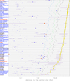 |
Fig. 5 Architecture of the 100 tightest planet-hosting binaries. Blue circles show aPl, while yellow circles show ab. The radius of the blue circle is proportional to the estimated radius of the planet. The radius of the yellow circle is proportional to the cubic root of the mass ratio between the companion and the central star (for the sake of visibility, planet sizes have been inflated by a factor of 20 with respect to star sizes). For planets and stars, the horizontal purple line represents the radial excursion due to the object’s eccentricity. For systems for which the semi-major axis of the binary is unknown, we simply plot the projected separation between the stellar components. These cases are indicated with a ‘|’ symbol overlaid onto the companion star. The black vertical bars between the planet and the stellar companion show the outer limit, acrit, for long-term orbital stability as estimated with the empirical formula of Holman & Wiegert (1999). When only the projected separation (ρb) of the binary is known, then the black bar represents acrit for a system with ab = ρb and eb = 0, while an additional green bar shows acrit assuming a ‘statistical’ binary orbit (log(ab) = log(ρb) + 0.13 and eb = 0.45), and an additional blue bar represents a ‘high-eccentricity’ case with ab = ρb and eb = 0.7. Systems detected by the RV method are written in black, those detected by transit are in blue, and those detected by other methods are in red. For systems where a brown dwarf exists in addition to planet(s), the BD location is plotted in orange. |
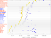 |
Fig. 6 Architecture of the 31 circumbinary planetary systems known to date. We note that we plot here, for both the companion star and the planet(s), the semi-major axis centred on the binary’s centre of mass. |
3.6 Circumbinary systems
Even if the main focus of this study is first and foremost binaries with S-type orbits, we also compiled a database of all known circumbinary (P-type) systems, which we present in Table B.1 and illustrate in Fig. 6. The size of this sample is much more limited, as there are only 31 circumbinary planetary systems known to date, more than 20 times less than in our main S-type database. Adding these systems to the 728 S-type binaries thus only marginally changes the global multiplicity fraction, which increases from 16.1% to 16.7% and from 22.5% to 23.0% for the db ≤ 500 domain.
As mentioned in the previous section, four of these circumbinaries also host a more distant stellar companion and are hierarchical triples for which the planet is both on a P-type and an S-type orbit. Interestingly, 4 out of 31 gives an S-type multiplicity fraction of ~13%, which is roughly comparable to our global S-type multiplicity rate of 16.1%, even if this conclusion suffers from obvious small number statistics.
4 Discussion
In the previous section, we argued that despite the heterogeneity of the sources our database is built on, some robust statistical results and trends can be derived. This is notably the case for the deficit of planet-hosting close-in binaries and the reliability of the global multiplicity fraction we derived in the db < 500 domain. In this section, we discuss these important issues in more detail.
4.1 Deficit of close-in binaries
The lack of close-in companion stars displayed in Fig. 1 is a feature that has been identified in numerous previous surveys of planet-hosting multiples (Wang et al. 2014; Kraus et al. 2016; Mugrauer 2019; Ziegler et al. 2020). Even if such a deficit makes sense from a theoretical point of view, because of the expected detrimental effect of close companions on the planet-formation process (Thebault & Haghighipour 2015), there is an ongoing debate as to whether or not this observed feature is due to observational biases or not (see Sect. 1). We argue that Fig. 2, which shows that the lower envelope of the (θb,db) distribution is not horizontal, convincingly demonstrates that the close-binary deficit cannot be entirely due to biases. This is because the two major biases potentially affecting our sample, namely the adverse selection effect against tight binaries in RV surveys (Hirsch et al. 2021) and the difficulty of finding close companions around planet-hosts in deep imaging surveys (Kraus et al. 2016), depend not on the physical separation (ρb) between binary components but on their on-sky angular separation (θb). This would lead to a horizontal lower envelope in a (θb, d) graph, which is clearly not the case. One could argue that this non-horizontal lower envelope is due to the fact that the (θb,db) graph is dominated by RV systems (black dots) at small db and transit systems (blue dots) at large db and to the fact that the different biases affecting these two different populations lead to a jump at the interface between the two distance domains. However, it is easy to see that the non-horizontal envelope is observed even when only restricting the sample to RV systems or when only considering transit systems. In addition, not only is the lower envelope non-horizontal, but it almost follows a diagonal ρb=cst line, which is what would be expected if the depletion of close binaries was a real physical feature. This analysis expands on the argument made by Ziegler et al. (2020) that the depletion of close-in companions must be real because it is of comparable amplitude for KOIs and TOIs despite the fact that Kepler targets are located at larger distances.
Of course, we are aware that our sample cannot be fully bias-free and that some of the lack of close-in binaries is due to adverse selection effects and limits to companion-seeking imaging searches, but it cannot account for all of it. In contrast, it is almost certain that the lack of wide separation binaries in the (db ≥ 500 pc, θb ≥2″) upper right-hand corner of Fig. 2 is a fully artificial feature. It likely results from the fact that two of the largest companion-searching surveys, Mugrauer (2019) and Michel & Mugrauer (2024), which account for roughly 40% of our sample, were limited to db ≤ 500–600 pc (because of precision limits on Gaia DR2 + DR3 parallax and proper motion measurements) and that most objects beyond 500 pc come from the surveys by Hirsch et al. (2017) and Sullivan et al. (2023, 2024), which vetted numerous stellar companion candidates identified in Furlan et al. (2017) but only for a on-sky separation of θb ≤2″.
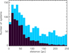 |
Fig. 7 Number of planet-hosting systems as a function of distance for the whole sample of 4504 systems listed in https://exoplanet.eu/. Blue is for transit-detected planets, and deep purple is for RV planets. |
4.2 Multiplicity fraction at d < 500 pc
A similar argument can be made with respect to the fM versus db distribution (shown in Fig. 3) not being bias dominated. Indeed, the fact that the two major adverse biases affecting binary statistics become more pronounced with a decreasing θb should mathematically lead to smaller fM values at larger distances in a bias-dominated sample. Granted, such a decrease is observed, but only in the db > 500 pc region. In the db ≲ 500 pc domain, fM is almost constant, thus strongly supporting that, even if a bias is present, it is not strong enough to skew the global fM statistics in this domain.
As with the separation distribution, this does not imply that our sample is bias-free, even at <500 pc. As an example, a 50 au physically separated binary is highly likely to be excluded from RV surveys if it is farther than ~50 pc, corresponding to an on-sky separation of ≤1″. We note, however, that the vast majority of RV-detected systems are relatively close, with ~70% of them lying at less than 60 pc, and that the population of exoplanets is largely dominated by transiting planets beyond this distance (Fig. 7). Therefore, the RV systems significantly affect the global value of fM(db) only in a distance domain where the selection bias, albeit real, is relatively limited. In addition, the ~1–2″ limit for excluding stellar companions is in fact not an absolute rule in RV surveys. When the magnitude difference (ΔM) between the stellar components is higher than ~3–4, the signal pollution by the companion becomes small enough to allow for correct RV analysis even when the companion is closer than 1″ (Eggenberger et al. 2007). This is the explanation for most of the planets detected by RV in ≲25 au binaries, such as HIP 90988, HD 72892, HD 144899, HD 28192, HD 199509, and HD 145934. In some rare cases, RV detections are even possible in tight binaries with ΔM < 3 (e.g. HD 196885, HD 87646).
Having identified the ≲500 pc domain as providing more reliable (if not fully bias-free) statistics, we could use this domain to derive more accurate results regarding the separation distribution of planet-hosting binaries. Fig. 8 shows the fraction, fM(ab), of planet-hosting stars that have a stellar companion with a given semi-major axis for both the total sample and the volume-limited db ≤ 500 pc sample, as compared to the empirical distribution for field stars derived by Raghavan et al. (2010). It can be seen that while the fM(ab) curve for the whole sample always stays below that of field stars, the distribution of fM(ab) in the db ≤ 500 pc domain becomes comparable to that of field stars for ab ≳300–500 au5. This is a clear indication of the completeness of the search for stellar companions to planet-hosts, at least for wide companions. It also strongly suggests that the deficit of planet-hosting close-in binaries could extend to separations of ~300–500 au.
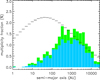 |
Fig. 8 Fraction, fM(ab), of planet-hosting stars that have a stellar companion in a given semi-major axis range. The blue histogram corresponds to the whole population of planet-hosting binaries, while the green one was computed for systems at a distance of less than 500pc. Values of fM(ab) were calculated by dividing the number of systems in each ab bin by the total number (or the total number at db ≤ 500 au) of planet-hosting stars found in the https://exoplanet.eu/ database. The black segments represent the multiplicity fraction distribution for the canonical binary distribution of Raghavan et al. (2010). We note that contrary to Fig. 1, here the Raghavan et al. (2010) distribution has not been normalised, and thus it allows for direct comparison to our database. |
4.3 Accounting for completeness issues
Our main result that the deficit of planet-hosting companions at ≲ 500 au separations cannot be fully explained by biases is essentially based on a visual analysis of the angle versus distance (Fig. 2) and fM versus distance (Fig. 3) plots. Another, and in principle more reliable (and more direct), way to derive this result would have been to accurately quantify all the observational biases (completeness and detection limits) affecting our database in order to debias it and compare it to the characteristics of field binaries. Unfortunately, the extreme diversity and heterogeneity of observational sources used in constructing the database prevented us from carrying out this procedure. Even when only considering surveys that have provided more than 10 objects, there are still 21 different observational sources left, each with its own specific detection limits and target-selection policy. In addition, there are the complex (and frequent) cases for which the companion stars have been visually detected in an AO or Speckle imaging survey but have been confirmed as bound companions in one or several later studies, whose limitations and target-selection policy also have to be factored into the bias estimate.
We did make an attempt at partially assessing the level of bias by focusing on the several surveys that have mined the Gaia catalogue, which have relatively coherent detection limits. This is especially true for the series of surveys that Mugrauer and collaborators published since 2019, which make up almost 40% of our database, for which we assumed the empirical detection limit, ΔM(θ), derived by Mugrauer et al. (2022), where ΔM is the magnitude difference between the binary components and θ is their angular separation (see Fig. 3 of Michel & Mugrauer 2024). We then used a Monte Carlo scheme to generate a sample of 105 binaries following the canonical distribution for field binaries by Raghavan et al. (2010) and the target distance distribution displayed in Fig. 1 of Michel & Mugrauer (2024), and we retained only those satisfying the aforementioned detection limit. Fig. 9 presents the obtained separation distribution for this sample, and in the figure we compare it to the distribution for the ‘MG’ subsample of companions obtained by Mugrauer (2019), Michel & Mugrauer (2021), and Michel & Mugrauer (2024). It can be seen that while the two distribution profiles do approximately match in the ≳1000 au domain, there is a significant lack of short separation binaries for the MG subsample as compared to what would be expected for an observationally biased field binary population. The Monte Carlo population peaks at a separation of ~500 au, while the MG subsample peaks around 2000 au. Using a bootstrap resampling procedure on the MG subsample, we found that its mean separation is comprised between 1645 and 2432 au at a confidence level of 3σ on the logarithmic distribution of separations. It is thus statistically different from that of the Monte-Carlo-generated population, whose average separation (calculated from the logarithmic distribution) is 727 au. Furthermore, there are only four planet-hosting binaries with ab ≤ 100 au in our MG subsample, when we should have had ~56 such systems for a canonical Raghavan et al. (2010) distribution (Fig. 9).
This analysis confirms that, for this important subsample of the database, the population of planet-hosting binaries physically differs from that of field binaries. However, it is also clear that some observational bias is present, as indicated by the difference between the Monte Carlo distribution profile and that of the unbiased Raghavan et al. (2010) binary population displayed in Fig. 1.
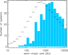 |
Fig. 9 Histogram (in blue) of the ab distribution for the subsample of Gaia-derived planet-hosting binaries obtained from Mugrauer (2019), Michel & Mugrauer (2021), and Michel & Mugrauer (2024). We also present the normalised ab distribution for a Monte Carlo generated population of field binaries following the canonical distribution of Raghavan et al. (2010) and the Gaia detection limit presented in Mugrauer et al. (2022). (See main text for details.) |
4.4 Stability and dynamical environment
The detailed study of individual systems is not the purpose of the present work. We present, however, in Fig. 5 a global view of the dynamical architecture of the tightest binaries in our sample. In particular, we show the location of the planet(s) with respect to the empirical orbital stability limit, acrit (Holman & Wiegert 1999). As discussed in Sect. 4.4, all but three planets are in the ‘safe’ ab ≤ acrit region, and even these three planets could in fact be on a stable orbit. It is, however, important to stress that the ab ≤ acrit criteria should only be taken as a first approximation and that precise orbital stability can only be assessed by means of thorough numerical exploration.
Going beyond the sole stability criteria, we note that a handful of planets, such as HIP 90988b, HD 41004Ab, TOI1736c, HD 196885b, γ Ceph b, GJ9714b, and HD 217958b (all of which are giants), orbit at locations that are below acrit but relatively close to it (Fig. 5). Thus, even if their orbits are stable, their dynamical environment is strongly perturbed by the companion star. Investigating planet formation processes in binaries goes far beyond the scope of the present paper, but it is highly likely that the presence of a companion star strongly perturbed the formation of these planets. As briefly mentioned in Sect. 1, the formation stage that is probably most affected by binary perturbations is the planetesimal accretion phase, as it requires a dynamically quiet environment with low enough impact velocities. Quantifying this detrimental effect is, however, a (very) arduous task, as it depends on the complex interplay between several mechanisms, such as binary secular perturbations, gas friction, disc self-gravity, or collisional output prescriptions (Marzari & Thebault 2019). Several analytical and numerical studies have nevertheless investigated this issue, but they often have conflicting conclusions regarding the detrimental effect of binarity (see, for instance, Thebault et al. 2008; Paardekooper et al. 2008; Xie & Zhou 2009; Xie et al. 2011; Fragner et al. 2011; Rafikov 2013; Silsbee & Rafikov 2021). Explaining the presence of giant planets in the dynamically highly perturbed environment close to acrit thus remains an open issue. Furthermore, planet formation in binaries has so far only been investigated in the context of the ‘classical’ incremental core-accretion scenario, in which kilometre-sized planetesimals slowly form from the local mutual sticking of smaller grains and in turn grow by mutual gravity during two-body impacts (e.g. Lissauer 1993). To our knowledge, no study has attempted to explore the new paradigm of planet formation that has emerged in recent years and the role of, for instance, streaming instability (e.g. Johansen et al. 2015), pebble accretion (Johansen & Lambrechts 2017), or snow-line induced pressure bumps (Izidoro et al. 2022) in the context of binarity. We believe that our database could be of great use for future studies investigating these issues. It could be exploited to test these mechanisms observationally and, in particular, the predictions they make regarding the correlations between binary separations and some other key observables, especially planetary masses and planetary locations.
5 Summary and conclusion
We have compiled the most extensive database of planet-hosting multiple systems (mainly binaries) ever assembled. This database currently lists the main characteristics (e.g. binary orbit or projected separation, distance, stellar masses, number of planets, stability limits for planets) of 728 S-type (circum-primary or circum-secondary) and 31 P-type (circumbinary) systems. It is made available to the community in an online version that will be regularly updated.
The heterogeneity of the sources this database is built on and the different observational biases that affect them represent a clear challenge for deriving precise statistical correlations. Nonetheless, some important qualitative trends and results can be derived. We confirm that the raw separation distribution of planet-hosting binaries shows a pronounced deficit of close-in companions. When plotting the distribution of binary angular separations as a function of system distance (db), we observed a non-horizontal lower envelope that indicates that this deficit of planet-hosting close-in binaries cannot be entirely due to adverse observational biases. We also showed that the multiplicity fraction (fM) among planet-hosting stars does not vary with system distance up to db ~ 500 pc, indicating that the subsample of db ≲ 500 pc planet-hosting binaries is not bias dominated (though it is not bias-free). For this subsample, we find fM = 22.5%, which is roughly half the multiplicity fraction of solar-type field stars, and it gives a first-order estimate of the detrimental effect binarity has on planet formation. For the same db ≲ 500 pc subsample, we find that the distribution of the multiplicity fraction, fM(ab), as a function of binary separation closely matches that of field stars beyond ~300–500 au, indicating that the search for stellar companions to planet-hosting stars is mostly complete at these separations. It also strongly suggests that the detrimental effect of binarity on planet formation can be felt up to separations of ~500 au.
Appendix A Sources used in compiling the database
Non-exhaustive list of main past surveys, looking for (or inventorying) stellar companions to exoplanet-hosts, used in compiling our database of systems with "S-type" configurations.
Appendix B Circumbinary database
Database of planet-hosting "P-type" (circumbinary) binaries, sorted by increasing binary separation. This is just an excerpt of the full table that is available, in a machine-readable form, at this URL: https://exoplanet.eu/planets_binary_circum/.
Appendix C Notes and references on S-type planet-hosting binaries
Notes and references for each individual system of the S-type database. This is only a highlight of the full notes that can be accessed at the following URL: https://exoplanet.eu/planets_binary_notes/.
Appendix D Notes and references on P-type (circumbinary) planet-hosting binaries
Notes and references for each individual system of the P-type (circumbinary) database. This is only a highlight of the full notes that can be accessed at the following URL: https://exoplanet.eu/planets_binary_notescirc/.
References
- Adams, E. R., Ciardi, D. R., Dupree, A. K., et al. 2012, AJ, 144, 42 [Google Scholar]
- Adams, E. R., Dupree, A. K., Kulesa, C., & McCarthy, D. 2013, AJ, 146, 9 [NASA ADS] [CrossRef] [Google Scholar]
- Baranec, C., Ziegler, C., Law, N. M., et al. 2016, AJ, 152, 18 [NASA ADS] [CrossRef] [Google Scholar]
- Barbato, D., Ségransan, D., Udry, S., et al. 2023, A&A, 674, A114 [NASA ADS] [CrossRef] [EDP Sciences] [Google Scholar]
- Beatty, T. G., Pepper, J., Siverd, R. J., et al. 2012, ApJ, 756, L39 [Google Scholar]
- Benedict, G. F., Harrison, T. E., Endl, M., & Torres, G. 2018, RNAAS, 2, 7 [NASA ADS] [Google Scholar]
- Beuermann, K., Hessman, F. V., Dreizler, S., et al. 2010, A&A, 521, L60 [NASA ADS] [CrossRef] [EDP Sciences] [Google Scholar]
- Bonavita, M., & Desidera, S. 2007, A&A, 468, 721 [NASA ADS] [CrossRef] [EDP Sciences] [Google Scholar]
- Borkovits, T., Hajdu, T., Sztakovics, J., et al. 2016, MNRAS, 455, 4136 [Google Scholar]
- Buchhave, L. A., Latham, D. W., Carter, J. A., et al. 2011, ApJS, 197, 3 [Google Scholar]
- Chabrier, G., Baraffe, I., Phillips, M., & Debras, F. 2023, A&A, 671, A119 [NASA ADS] [CrossRef] [EDP Sciences] [Google Scholar]
- Chauvin, G., Lagrange, A. M., Udry, S., et al. 2006, A&A, 456, 1165 [NASA ADS] [CrossRef] [EDP Sciences] [Google Scholar]
- Chauvin, G., Videla, M., Beust, H., et al. 2023, A&A, 675, A114 [NASA ADS] [CrossRef] [EDP Sciences] [Google Scholar]
- Colton, N. M., Horch, E. P., Everett, M. E., et al. 2021, AJ, 161, 21 [Google Scholar]
- Conroy, K. E., Prša, A., Stassun, K. G., et al. 2014, AJ, 147, 45 [NASA ADS] [CrossRef] [Google Scholar]
- Desidera, S., & Barbieri, M. 2007, A&A, 462, 345 [NASA ADS] [CrossRef] [EDP Sciences] [Google Scholar]
- Duquennoy, A., & Mayor, M. 1991, A&A, 248, 485 [NASA ADS] [Google Scholar]
- Eggenberger, A., Udry, S., Chauvin, G., et al. 2007, A&A, 474, 273 [NASA ADS] [CrossRef] [EDP Sciences] [Google Scholar]
- Eggenberger, A., Udry, S., Chauvin, G., et al. 2011, in IAU Symposium, 276, The Astrophysics of Planetary Systems: Formation, Structure, and Dynamical Evolution, eds. A. Sozzetti, M. G. Lattanzi, & A. P. Boss, 409 [Google Scholar]
- Evans, D. F., Southworth, J., Maxted, P. F. L., et al. 2016, A&A, 589, A58 [NASA ADS] [CrossRef] [EDP Sciences] [Google Scholar]
- Evans, D. F., Southworth, J., Smalley, B., et al. 2018, A&A, 610, A20 [NASA ADS] [CrossRef] [EDP Sciences] [Google Scholar]
- Fontanive, C., & Bardalez Gagliuffi, D. 2021, Front. Astron. Space Sci., 8, 16 [NASA ADS] [CrossRef] [Google Scholar]
- Fragner, M. M., Nelson, R. P., & Kley, W. 2011, A&A, 528, A40 [NASA ADS] [CrossRef] [EDP Sciences] [Google Scholar]
- Furlan, E., Ciardi, D. R., Everett, M. E., et al. 2017, AJ, 153, 71 [NASA ADS] [CrossRef] [Google Scholar]
- Ginski, C., Mugrauer, M., Seeliger, M., et al. 2016, MNRAS, 457, 2173 [Google Scholar]
- González-Payo, J., Caballero, J. A., Gorgas, J., et al. 2024, A&A, 689, A302 [NASA ADS] [CrossRef] [EDP Sciences] [Google Scholar]
- Gould, A., Udalski, A., Shin, I. G., et al. 2014, Science, 345, 46 [CrossRef] [Google Scholar]
- Hirsch, L., Ciardi, D. R., Howard, A. W., et al. 2017, AJ, 153, 117 [NASA ADS] [CrossRef] [Google Scholar]
- Hirsch, L., Rosenthal, L., Fulton, B. J., et al. 2021, AJ, 161, 134 [NASA ADS] [CrossRef] [Google Scholar]
- Holman, M., & Wiegert, P. 1999, AJ, 117, 621 [CrossRef] [Google Scholar]
- Horch, E. P., Howell, S. B., Everett, M. E., & Ciardi, D. R. 2014, ApJ, 795, 60 [NASA ADS] [CrossRef] [Google Scholar]
- Howard, A. W., Johnson, J. A., Marcy, G. W., et al. 2010, ApJ, 721, 1467 [Google Scholar]
- Howell, S. B., Everett, M. E., Sherry, W., Horch, E., & Ciardi, D. R. 2011, AJ, 142, 19 [Google Scholar]
- Izidoro, A., Dasgupta, R., Raymond, S. N., et al. 2022, Nat. Astron., 6, 357 [NASA ADS] [CrossRef] [Google Scholar]
- Janson, M., Gratton, R., Rodet, L., et al. 2021, Nature, 600, 231 [NASA ADS] [CrossRef] [Google Scholar]
- Jing, Y., Mao, T.-X., Wang, J., Liu, C., & Chen, X. 2025, ApJS, 277, 15 [Google Scholar]
- Johansen, A., & Lambrechts, M. 2017, Annu. Rev. Earth Planet. Sci., 45, 359 [Google Scholar]
- Johansen, A., Mac Low, M.-M., Lacerda, P., & Bizzarro, M. 2015, Sci. Adv., 1, 1500109 [CrossRef] [Google Scholar]
- Kostov, V. B., McCullough, P. R., Hinse, T. C., et al. 2013, ApJ, 770, 52 [NASA ADS] [CrossRef] [Google Scholar]
- Kraus, A., Ireland, M., Huber, D., Mann, A., & Dupuy, T. 2016, AJ, 152, 8 [NASA ADS] [CrossRef] [Google Scholar]
- Lehmann, H., Borkovits, T., Rappaport, S. A., et al. 2016, ApJ, 819, 33 [Google Scholar]
- Lester, K. V., Howell, S. B., Matson, R. A., et al. 2023, AJ, 166, 166 [NASA ADS] [CrossRef] [Google Scholar]
- Lillo-Box, J., Barrado, D., & Bouy, H. 2012, A&A, 546, A10 [NASA ADS] [CrossRef] [EDP Sciences] [Google Scholar]
- Lillo-Box, J., Barrado, D., & Bouy, H. 2014, A&A, 566, A103 [NASA ADS] [CrossRef] [EDP Sciences] [Google Scholar]
- Lissauer, J. J. 1993, ARA&A, 31, 129 [NASA ADS] [CrossRef] [Google Scholar]
- Martin, D. V. 2018, Handbook of Exoplanets, eds. H. J. Deeg & J. A. Belmonte (Springer International Publishing AG) [Google Scholar]
- Marzari, F., & Thebault, P. 2019, Galaxies, 7, 84 [NASA ADS] [CrossRef] [Google Scholar]
- Mason, B. D., Wycoff, G. L., Hartkopf, W. I., Douglass, G. G., & Worley, C. E. 2001, AJ, 122, 3466 [Google Scholar]
- Matson, R. A., Howell, S. B., Horch, E. P., & Everett, M. E. 2018, AJ, 156, 31 [NASA ADS] [CrossRef] [Google Scholar]
- Michel, K. U., & Mugrauer, M. 2021, Front. Astron. Space Sci., 8, 14 [NASA ADS] [CrossRef] [Google Scholar]
- Michel, K.-U., & Mugrauer, M. 2024, MNRAS, 527, 3183 [Google Scholar]
- Morley, C. V., Mukherjee, S., Marley, M. S., et al. 2024, ApJ, 975, 59 [NASA ADS] [CrossRef] [Google Scholar]
- Mugrauer, M. 2019, MNRAS, 490, 5088 [Google Scholar]
- Mugrauer, M., & Neuhäuser, R. 2009, A&A, 494, 373 [NASA ADS] [CrossRef] [EDP Sciences] [Google Scholar]
- Mugrauer, M., & Michel, K.-U. 2020, Astron. Nachr., 341, 996 [NASA ADS] [CrossRef] [Google Scholar]
- Mugrauer, M., & Michel, K.-U. 2021, Astron. Nachr., 342, 840 [NASA ADS] [CrossRef] [Google Scholar]
- Mugrauer, M., Neuhäuser, R., Mazeh, T., et al. 2006, Astron. Nachr., 327, 321 [NASA ADS] [CrossRef] [Google Scholar]
- Mugrauer, M., Ginski, C., & Seeliger, M. 2014, MNRAS, 439, 1063 [Google Scholar]
- Mugrauer, M., Zander, J., & Michel, K.-U. 2022, Astron. Nachr., 343, e24017 [NASA ADS] [Google Scholar]
- Mugrauer, M., Rück, J., & Michel, K. U. 2023, Astron. Nachr., 344, e20230055 [Google Scholar]
- Müller, T., & Kley, W. 2012, A&A, 539, A18 [NASA ADS] [CrossRef] [EDP Sciences] [Google Scholar]
- Ngo, H., Knutson, H. A., Hinkley, S., et al. 2015, ApJ, 800, 138 [Google Scholar]
- Ngo, H., Knutson, H. A., Hinkley, S., et al. 2016, ApJ, 827, 8 [Google Scholar]
- Ngo, H., Knutson, H. A., Bryan, M. L., et al. 2017, AJ, 153, 242 [Google Scholar]
- Özdönmez, A., Er, H., & Nasiroglu, I. 2023, MNRAS, 526, 4725 [CrossRef] [Google Scholar]
- Paardekooper, S. J., Thebault, P., & Mellema, G. 2008, MNRAS, 386, 973 [NASA ADS] [CrossRef] [Google Scholar]
- Patience, J., White, R. J., Ghez, A. M., et al. 2002, ApJ, 581, 654 [NASA ADS] [CrossRef] [Google Scholar]
- Pilat-Lohinger, E. 2005, in IAU Colloq. 197: Dynamics of Populations of Planetary Systems, eds. Z. Knežević & A. Milani, 71 [Google Scholar]
- Poleski, R., Skowron, J., Udalski, A., et al. 2014, ApJ, 795, 42 [Google Scholar]
- Qian, S. B., Liao, W. P., Zhu, L. Y., & Dai, Z. B. 2010, ApJ, 708, L66 [CrossRef] [Google Scholar]
- Rafikov, R. R. 2013, ApJ, 765, L8 [Google Scholar]
- Raghavan, D., Henry, T. J., Mason, B. D., et al. 2006, ApJ, 646, 523 [NASA ADS] [CrossRef] [Google Scholar]
- Raghavan, D., McAlister, H. A., Henry, T. J., et al. 2010, ApJS, 190, 1 [Google Scholar]
- Rizzuto, A. C., Ireland, M. J., Robertson, J. G., et al. 2013, MNRAS, 436, 1694 [Google Scholar]
- Roell, T., Neuhäuser, R., Seifahrt, A., & Mugrauer, M. 2012, A&A, 542, A92 [NASA ADS] [CrossRef] [EDP Sciences] [Google Scholar]
- Savonije, G., Papaloizou, J., & Lin, D. N. C. 1994, MNRAS, 268, 13 [NASA ADS] [CrossRef] [Google Scholar]
- Schlagenhauf, S., Mugrauer, M., Ginski, C., et al. 2024, MNRAS, 529, 4768 [Google Scholar]
- Schneider, J., Dedieu, C., Le Sidaner, P., Savalle, R., & Zolotukhin, I. 2011, A&A, 532, A79 [NASA ADS] [CrossRef] [EDP Sciences] [Google Scholar]
- Schwamb, M. E., Orosz, J. A., Carter, J. A., et al. 2013, ApJ, 768, 127 [Google Scholar]
- Silsbee, K., & Rafikov, R. 2021, A&A, 652, A104 [NASA ADS] [CrossRef] [EDP Sciences] [Google Scholar]
- Sullivan, K., Kraus, A. L., Huber, D., et al. 2023, AJ, 165, 177 [NASA ADS] [Google Scholar]
- Sullivan, K., Kraus, A. L., Berger, T. A., et al. 2024, AJ, 168, 129 [Google Scholar]
- Thebault, P. 2011, Celest. Mech. Dyn. Astron., 111, 29 [NASA ADS] [CrossRef] [Google Scholar]
- Thebault, P., & Haghighipour, N. 2015, in Planetary Exploration and Science: Recent Results and Advances, eds. S. Jin, N. Haghighipour, & W.-H. Ip, 309 [Google Scholar]
- Thebault, P., Marzari, F., & Scholl, H. 2006, Icarus, 183, 193 [NASA ADS] [CrossRef] [Google Scholar]
- Thebault, P., Marzari, F., & Scholl, H. 2008, MNRAS, 388, 1528 [Google Scholar]
- Trifonov, T., Lee, M. H., Reffert, S., & Quirrenbach, A. 2018, AJ, 155, 174 [Google Scholar]
- Wang, J., Fischer, D. A., Xie, J.-W., & Ciardi, D. R. 2014, ApJ, 791, 111 [CrossRef] [Google Scholar]
- Wang, J., Fischer, D. A., Horch, E. P., & Xie, J.-W. 2015, ApJ, 806, 248 [NASA ADS] [CrossRef] [Google Scholar]
- Xie, J.-W., & Zhou, J.-L. 2009, ApJ, 698, 2066 [Google Scholar]
- Xie, J.-W., Payne, M. J., Thebault, P., Zhou, J.-L., & Ge, J. 2011, ApJ, 735, 10 [Google Scholar]
- Ziegler, C., Law, N. M., Morton, T., et al. 2017, AJ, 153, 66 [NASA ADS] [CrossRef] [Google Scholar]
- Ziegler, C., Law, N. M., Baranec, C., et al. 2018, AJ, 156, 83 [Google Scholar]
- Ziegler, C., Tokovinin, A., Briceño, C., et al. 2020, AJ, 159, 19 [Google Scholar]
- Ziegler, C., Tokovinin, A., Latiolais, M., et al. 2021, AJ, 162, 192 [NASA ADS] [CrossRef] [Google Scholar]
Histograms produced with different prescriptions between projected separation, ρb, and real semi-major axis, ab, do not lead to statistically different results. As an example, the extreme case ab = ρb leads to ![Mathematical equation: $\[<a_{b}>=686_{-79}^{+117}\]$](/articles/aa/full_html/2025/08/aa55457-25/aa55457-25-eq2.png) au.
au.
The difference between fM values in the d ≤ 500 au and d ≥ 500 au domains is statistically significant, with the 3σ error bars being ![Mathematical equation: $\[<f_{M}>_{d<500}=0.225_{-0.012}^{+0.013}\]$](/articles/aa/full_html/2025/08/aa55457-25/aa55457-25-eq3.png) and
and ![Mathematical equation: $\[<f_{M}>_{d>500}=0.120_{-0.025}^{+0.027}\]$](/articles/aa/full_html/2025/08/aa55457-25/aa55457-25-eq4.png) .
.
One could argue that the match beyond ab ≳300–500 au is not perfect, with an excess of companions in the 1000–5000 au range and a deficit of companions beyond ~10 000 au, but these features are actually also observed for field stars; the empirical law derived by Raghavan et al. (2010) indeed underestimates fM(ab) for 1000 ≲ ab ≲ 5000 au and overestimates it beyond ~10 000 au (see Fig. 13 of that paper).
All Tables
Complete database of planet-hosting ‘S-type’ binaries, sorted by increasing binary separation.
Multiplicity fraction (fM) for the whole population of exoplanet hosts as well as a function of stellar type (for the planet-bearing star).
Planet semi-major axis (aPl) and projected separations (ρAB and ρAC) of the stellar companions for the three non-hierarchical planetbearing triples.
Non-exhaustive list of main past surveys, looking for (or inventorying) stellar companions to exoplanet-hosts, used in compiling our database of systems with "S-type" configurations.
Database of planet-hosting "P-type" (circumbinary) binaries, sorted by increasing binary separation. This is just an excerpt of the full table that is available, in a machine-readable form, at this URL: https://exoplanet.eu/planets_binary_circum/.
Notes and references for each individual system of the S-type database. This is only a highlight of the full notes that can be accessed at the following URL: https://exoplanet.eu/planets_binary_notes/.
Notes and references for each individual system of the P-type (circumbinary) database. This is only a highlight of the full notes that can be accessed at the following URL: https://exoplanet.eu/planets_binary_notescirc/.
All Figures
|
Fig. 1 Histogram of planet-hosting binary semi-major axis for the complete sample. When only the projected separation (ρb) is known, a ‘statistical’ semi-major axis is considered following the relation derived by Duquennoy & Mayor (1991) for randomly distributed orbits (see text for details). The black line corresponds to the normalised distribution for field stars derived by Raghavan et al. (2010). |
| In the text | |
|
Fig. 2 On-sky projected angular separation (θb) between binary components as a function of distance (db) to the system. The four black lines correspond (from bottom to top) to physical separations of 10, 100, 1000, and 10 000 au. We note that Proxima Centauri has been left out of this graph in order not to ‘squeeze’ the graph’s Y-axis. |
| In the text | |
|
Fig. 3 Multiplicity fraction of confirmed planet hosts as a function of distance to the system. |
| In the text | |
|
Fig. 4 Fraction of planet-hosting primaries (blue) and stellar companions (deep purple) in our database as a function of stellar type. The red histogram corresponds to the distribution for planet-hosting single stars (taken from the Encyclopaedia of Exoplanetary Systems). |
| In the text | |
|
Fig. 5 Architecture of the 100 tightest planet-hosting binaries. Blue circles show aPl, while yellow circles show ab. The radius of the blue circle is proportional to the estimated radius of the planet. The radius of the yellow circle is proportional to the cubic root of the mass ratio between the companion and the central star (for the sake of visibility, planet sizes have been inflated by a factor of 20 with respect to star sizes). For planets and stars, the horizontal purple line represents the radial excursion due to the object’s eccentricity. For systems for which the semi-major axis of the binary is unknown, we simply plot the projected separation between the stellar components. These cases are indicated with a ‘|’ symbol overlaid onto the companion star. The black vertical bars between the planet and the stellar companion show the outer limit, acrit, for long-term orbital stability as estimated with the empirical formula of Holman & Wiegert (1999). When only the projected separation (ρb) of the binary is known, then the black bar represents acrit for a system with ab = ρb and eb = 0, while an additional green bar shows acrit assuming a ‘statistical’ binary orbit (log(ab) = log(ρb) + 0.13 and eb = 0.45), and an additional blue bar represents a ‘high-eccentricity’ case with ab = ρb and eb = 0.7. Systems detected by the RV method are written in black, those detected by transit are in blue, and those detected by other methods are in red. For systems where a brown dwarf exists in addition to planet(s), the BD location is plotted in orange. |
| In the text | |
|
Fig. 6 Architecture of the 31 circumbinary planetary systems known to date. We note that we plot here, for both the companion star and the planet(s), the semi-major axis centred on the binary’s centre of mass. |
| In the text | |
|
Fig. 7 Number of planet-hosting systems as a function of distance for the whole sample of 4504 systems listed in https://exoplanet.eu/. Blue is for transit-detected planets, and deep purple is for RV planets. |
| In the text | |
|
Fig. 8 Fraction, fM(ab), of planet-hosting stars that have a stellar companion in a given semi-major axis range. The blue histogram corresponds to the whole population of planet-hosting binaries, while the green one was computed for systems at a distance of less than 500pc. Values of fM(ab) were calculated by dividing the number of systems in each ab bin by the total number (or the total number at db ≤ 500 au) of planet-hosting stars found in the https://exoplanet.eu/ database. The black segments represent the multiplicity fraction distribution for the canonical binary distribution of Raghavan et al. (2010). We note that contrary to Fig. 1, here the Raghavan et al. (2010) distribution has not been normalised, and thus it allows for direct comparison to our database. |
| In the text | |
|
Fig. 9 Histogram (in blue) of the ab distribution for the subsample of Gaia-derived planet-hosting binaries obtained from Mugrauer (2019), Michel & Mugrauer (2021), and Michel & Mugrauer (2024). We also present the normalised ab distribution for a Monte Carlo generated population of field binaries following the canonical distribution of Raghavan et al. (2010) and the Gaia detection limit presented in Mugrauer et al. (2022). (See main text for details.) |
| In the text | |
Current usage metrics show cumulative count of Article Views (full-text article views including HTML views, PDF and ePub downloads, according to the available data) and Abstracts Views on Vision4Press platform.
Data correspond to usage on the plateform after 2015. The current usage metrics is available 48-96 hours after online publication and is updated daily on week days.
Initial download of the metrics may take a while.