| Issue |
A&A
Volume 700, August 2025
|
|
|---|---|---|
| Article Number | A282 | |
| Number of page(s) | 20 | |
| Section | Stellar structure and evolution | |
| DOI | https://doi.org/10.1051/0004-6361/202555502 | |
| Published online | 28 August 2025 | |
Evolving magnetic lives of Sun-like stars
I. Characterisation of the large-scale magnetic field with Zeeman-Doppler imaging
1
Leiden Observatory, Leiden University, PO Box 9513
2300
RA, Leiden, The Netherlands
2
Institut de Recherche en Astrophysique et Planétologie, Université de Toulouse, CNRS, IRAP/UMR 5277, 14 avenue Edouard Belin, F-31400
Toulouse, France
3
Science Division, Directorate of Science, European Space Research and Technology Centre (ESA/ESTEC), Keplerlaan 1, 2201
AZ, Noordwijk, The Netherlands
4
University of Vienna, Department of Astrophysics, Türkenschanzstrasse 17, A-1180
Vienna, Austria
5
Tartu Observatory, University of Tartu, Observatooriumi 1, Tõravere, 61602
Estonia
6
Laboratoire Univers et Particules de Montpellier, Université de Montpellier, CNRS, F-34095
Montpellier, France
7
Univ. Grenoble Alpes, CNRS, IPAG, 38000
Grenoble, France
⋆ Corresponding author: This email address is being protected from spambots. You need JavaScript enabled to view it.
Received:
13
May
2025
Accepted:
14
July
2025
Abstract
Context. Planets orbiting young, solar-type stars are embedded in a more energetic environment than that of the solar neighbourhood. They experience harsher conditions due to enhanced stellar magnetic activity and wind shaping the secular evolution of a planetary atmosphere.
Aims. This study is dedicated to the characterisation of the magnetic activity of eleven Sun-like stars, with ages between 0.2 and 6.1 Gyr and rotation periods between 4.6 and 28.7 d. Based on a sub-sample of six stars, we aim to study the large-scale magnetic field, which we then use to simulate the associated stellar wind and environment. Finally, we want to determine the conditions during the early evolution of planetary habitability.
Methods. We analysed high-resolution spectropolarimetric data collected in 2018 and 2019 with Narval. We computed activity diagnostics from chromospheric lines such as Ca II H&K, Hα, and the Ca II infrared triplet, as well as the longitudinal magnetic field from circularly polarised least-squares deconvolution profiles. For six stars exhibiting detectable circular polarisation signals, we reconstructed the large-scale magnetic field at the photospheric level by means of Zeeman-Doppler imaging (ZDI).
Results. In agreement with previous studies, we found a global decrease in the activity indices and longitudinal field with increasing age and rotation period. The large-scale magnetic field of the six sub-sample stars displays a strength between 1 and 25 G and reveals substantial contributions from different components such as poloidal (40–90%), toroidal (10–60%), dipolar (30–80%), and quadrupolar (10–40%), with distinct levels of axisymmetry (6–84%) and short-term variability of the order of months. Ultimately, this implies that exoplanets tend to experience a broad variety of stellar magnetic environments after their formation.
Key words: techniques: polarimetric / stars: activity / stars: magnetic field
© The Authors 2025
 Open Access article, published by EDP Sciences, under the terms of the Creative Commons Attribution License (https://creativecommons.org/licenses/by/4.0), which permits unrestricted use, distribution, and reproduction in any medium, provided the original work is properly cited.
This article is published in open access under the Subscribe to Open model. This email address is being protected from spambots. You need JavaScript enabled to view it. to support open access publication.
1. Introduction
Stellar magnetic activity powers outflows and eruptive processes such as flares, coronal mass ejections, and energetic particle events. The collective action of these phenomena determines the space weather planets orbit within and plays a major role in the processing of planetary magnetospheres and upper atmospheres (e.g. Lammer et al. 2003, 2012; Rugheimer et al. 2015). Magnetic interactions in the outer stellar layers (chromosphere, transition region, and corona) produce energetic X-ray and extreme ultraviolet (EUV) radiation that can heat and ionise upper planetary atmospheres, triggering their evaporation and photochemistry (Cecchi-Pestellini et al. 2006; Murray-Clay et al. 2009; Owen & Jackson 2012; Tsai et al. 2023; Van Looveren et al. 2025). A similar effect is also induced by stellar cosmic rays (Rodgers-Lee et al. 2021a, 2021b; Raeside et al. 2025). Ultimately, the evolution of stellar activity during the history of a star dictates any observed planetary atmosphere (Penz & Micela 2008; Sanz-Forcada et al. 2011; Locci et al. 2019; Allan & Vidotto 2019). This is fundamental, for example, to explain the atmospheric evolution of Solar System planets (Lammer et al. 2003; Wood 2004; Kulikov et al. 2007; Airapetian & Usmanov 2016).
In this context, studying Sun-like stars at different ages is relevant to understanding planetary atmospheric evolution at early stages of formation, as well as the consequences of such extreme conditions for the habitability of Earth-like planets (See et al. 2014; Airapetian et al. 2020). Observations of young stars indicate an enhanced magnetic activity and a harsher space environment compared to the current Sun (Wood 2006), implying more frequent and more energetic phenomena (Wood 2004, 2006; Güdel 2007). For instance, X-ray and extreme ultraviolet (EUV) emission can be two or three orders of magnitude larger than in the case of our Sun (Guinan et al. 2003; Ribas et al. 2005; Tu et al. 2015; Johnstone et al. 2021; Ketzer & Poppenhaeger 2023).
The nature of stellar activity is dictated by the intensity and structure of the magnetic field, which, in turn, depends on the rotation and internal structure of the star. Knowing the intensity of the magnetic fields on young planetary host stars, which can be several tens to hundreds of times stronger than that of the Sun (e.g. Folsom et al. 2018), is a pivotal precondition to understanding whether planets can become habitable in the early evolution of a planetary system. Moreover, the habitability conditions are not solely determined by the star’s temperature, but also by its magnetic field (Vidotto et al. 2013; Cockell et al. 2016), which can influence the survival of the planetary atmosphere (see Fig. 5 in Van Looveren et al. 2025, for a recent example).
The level of stellar magnetic activity is evaluated via proxies such as photometric variability, X-ray luminosity, and emission in the cores of chromospheric lines. The latter are typically Ca II H&K, Hα, and Ca II infrared triplet lines (Wilson 1968; Gizis et al. 2002; Busà et al. 2007). A detailed characterisation of the stellar magnetic field can be carried out with spectropolarimetry, an observational technique that detects magnetically induced polarisation in spectral lines owing to the Zeeman effect (Zeeman 1897; Donati et al. 1997; Landstreet 2009). By collecting a time series of polarised spectra, it is possible to reconstruct the geometry of the large-scale magnetic field at the surface of the star by means of tomographic inversion, that is, Zeeman-Doppler imaging (ZDI; Semel 1989; Donati & Brown 1997). The resulting maps of the magnetic field can then be used as boundary conditions to extrapolate the field lines outward and model the stellar wind via magnetohydrodynamical simulations (e.g. Vidotto et al. 2014a, 2023; Nicholson et al. 2016; Boro Saikia et al. 2020; Folsom et al. 2020; Alvarado-Gómez et al. 2022; Evensberget et al. 2021, 2022, 2023).
The ZDI technique has been extensively applied to study the strength and configuration of the large-scale magnetic field of Sun-like stars of different ages and rotation periods (Donati & Collier Cameron 1997; Petit et al. 2008; Rosén et al. 2016; Folsom et al. 2016, 2018; Willamo et al. 2022). Distinct trends have emerged: for instance, slowly rotating Sun-like stars tend to exhibit poloidal-dominated field geometries, as shown by Petit et al. (2008) and Brown et al. (2022), together with a decrease in chromospheric activity. Furthermore, the average magnetic field strength decreases with increasing age and rotation period (e.g. Vidotto et al. 2014a; Folsom et al. 2018; Willamo et al. 2022), which is in agreement with trends of the total, unsigned magnetic field measurements performed by theoretical modelling of Zeeman broadening (Reiners 2012; Kochukhov et al. 2020). Repeated reconstructions of the large-scale magnetic field with ZDI have also revealed the presence of long-term trends and magnetic cycles for these stars (e.g. Fares et al. 2009; Rosén et al. 2016; Boro Saikia et al. 2016; Jeffers et al. 2017; Alvarado-Gómez et al. 2018; Bellotti et al. 2025).
In this work, we characterise the magnetic field and activity level for a sample of Sun-like stars whose ages span between 0.2 and 6.1 Gyr and with their rotation periods between 4.6 and 28.7 d. Thus, we are set to continue the exploration of magnetic activity properties across a wide stellar parameter space. For a sub-sample of six stars having detectable Zeeman signatures in circular polarisation and suitable temporal sampling of their rotation, we reconstructed the large-scale magnetic field geometry with ZDI. These six stars have ages between 0.2 and 1.6 Gyr and rotation periods between 4.6 and 12.4 d. In this age range, the relation between rotation period and age is not unique, thus, monitoring many stars in this age range is important. The magnetic field maps resulting from this study will be used in a subsequent work for stellar wind and environment modelling.
The paper is structured as follows. In Sect. 2, we describe the sample of Sun-like stars examined in this study and their spectropolarimetric observations performed with the high-resolution spectropolarimeter Narval. In Sect. 3, we outline the computation of canonical activity indices as well as the longitudinal magnetic field. In Sect. 4, we recall the principles and assumptions of ZDI. Finally, we discuss our results star-by-star and general trends in Sects. 5 and 6, presenting our conclusions in Sect. 7.
2. Observations
The targets of our study are 11 G-type stars. According to the literature, they exhibit considerably distinct activity levels, along with likely differences in the magnetic field structure, wind properties, and high-energy output. We placed our stars on the rotation evolutionary tracks of Tu et al. (2015) to highlight this point, as illustrated in Fig. 1. The cited authors showed how the temporal evolution of stellar rotation, along with the associated X-ray and EUV luminosity, has a significant impact on the atmospheric evolution of exoplanets. Our stellar sample covers the three rotational evolution tracks (slow, medium, and fast), providing good coverage of the non-unique rotational history of Sun-like stars during the first few hundred million years. The Sun could have taken any of these three paths, so this coverage of the rotational evolution is necessary to remark on the magnetic history of the Sun.
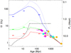 |
Fig. 1. Rotational evolutionary tracks computed by Johnstone et al. (2015a,b) and used in Tu et al. (2015), with our sample stars overplotted. Magenta data points indicate stars with a ZDI map both in the literature and presented in this work, cyan data points indicate stars with a first ZDI reconstruction in this work, and yellow data points indicate stars without a ZDI map. Some of the error bars are smaller than the data point size. The curves represent the 10th (red), 50th (green), and 90th (blue) percentiles of the stellar rotational distribution, of the envelope (solid lines) and core (dotted lines). The small horizontal lines are the observational constraints for the corresponding percentiles. The dashed black line is a time-dependent saturation relation for the stellar dipolar field, the wind mass loss rate and the X-ray luminosity. For more information, see the work of Tu et al. (2015). |
Four stars in our sample (HD 1835, HD 82443, HD 189733, and HD 206860) have already been observed with spectropolarimetry, but these observations date back to different epochs. Therefore, our analyses also address the evolution of the magnetic field structure on timescales of many years, as reported previously for other Sun-like stars (Donati et al. 2008; Boro Saikia et al. 2015; Rosén et al. 2016; Willamo et al. 2022; Bellotti et al. 2025).
The properties of our stars are summarised in Table 1. The ages of the stars were mostly extracted from the work of Ramírez et al. (2012) and Linsky et al. (2020). Furthermore, Ramírez et al. (2012) used either isochrones or gyrochronology to estimate the stellar age. The latter method is more accurate for young active stars. For our stars, the ages of HD 149026 and HD 219828 were obtained via isochrones, while for the remaining stars, ages were obtained from gyrochronology.
Properties of our stars.
We analysed optical spectropolarimetric observations collected with Narval in 2018 and 20191. Narval is the spectropolarimeter on the 2 m Télescope Bernard Lyot (TBL) at the Pic du Midi Observatory in France (Donati 2003), which operates between 370 and 1050 nm at high resolution (R = 65, 000). The observations were carried out in circular polarisation mode, providing both unpolarised (Stokes I) and circularly polarised (Stokes V) high-resolution spectra. The data were reduced with the LIBRE-ESPRIT pipeline (Donati et al. 1997) and the continuum-normalised spectra were retrieved from PolarBase (Petit et al. 2014). We provide the full list of observations in Table A.1 and the total number of observations for each star in Table B.1.
The detection and characterisation of Zeeman signatures in circularly polarised light are performed by means of least-squares deconvolution (LSD; Donati et al. 1997; Kochukhov et al. 2010) using the LSDPY code which is part of the Specpolflow software (Folsom et al. 2025)2. This numerical technique produces high signal-to-noise ratio (S/N) line profiles (unpolarised and circularly polarised) from the combination of thousands of photospheric spectral lines included in a synthetic line list. The line lists were produced using the Vienna Atomic Line Database3 (VALD, Ryabchikova et al. 2015). They contain information of atomic lines with known Landé factor (indicated by geff and describing the magnetic sensitivity of a spectral line) and with a depth greater than 40% the level of the unpolarised continuum (following Donati et al. 1997). A summary of the line lists used and their properties is given in Table B.1.
We recorded substantially lower S/N in Stokes V LSD profiles for two observations of HD 206860 on July 26th 2018 and June 22nd 2019, as well as for HD 43162 on December 19th 2018; hence, these observations were excluded from the analysis. For HD 206860, we also noticed that the Stokes V profile on July 28, 2018 featured several oscillations around the zero flux level and was also excluded. For three stars, namely, HD 149026, HD 190406, and HD 219828, we did not report any clear detections of Zeeman signatures in Stokes V profiles. Indeed, for each star, the false-alarm probability (FAP; see Donati et al. 1997, for more details) of the putative Zeeman signature is greater than 10−3. It was only in a couple of observations that we were able to see a marginal detection (FAP ∼ 10−3 − 10−4). For this reason, these stars were excluded from the spectropolarimetric characterisation analyses, however, they were retained for the measurement of unpolarised magnetic activity indicators, as outlined in the next sections. In Appendix B, we describe the polarisation signatures in Stokes V as well as spurious polarisation signatures in Stokes N. In the next following, the observations have been phased with the following ephemeris,
 (1)
(1)
where HJD0 is the heliocentric Julian Date reference (the first one of the time series for each star, see Table A.1), Prot is the rotation period of the star (see Table 1), and ncyc represents the rotation cycle.
3. Activity indices
To gauge the magnetic activity level of our stars, we computed time series of activity indices. We used chromospheric spectral lines falling in the optical domain covered by Narval, namely the Ca II H&K lines, Hα, and Ca II infrared triplet lines. In Table C.1, we list the main statistical features of the time series for all three activity indicators.
The logR′HK quantifies the amount of flux in the Ca II H&K lines relative to the nearby continuum, without colour dependence and photospheric contribution (Middelkoop 1982; Noyes et al. 1984; Rutten 1984). The recipe to compute the index consists of three steps: (i) measuring the S index, (ii) calibrating it to the Mount Wilson scale, and iii) converting it to the logR′HK index. Following the definition of Vaughan et al. (1978), the S index is measured via
 (2)
(2)
where FH and FK are the fluxes in two triangular band passes with FWHM = 1.09 Å centred on the cores of the H line (3968.470 Å) and K line (3933.661 Å), whereas FR and FV are the fluxes within two 20-Å rectangular band passes centred at 3901 and 4001 Å, respectively. The set of coefficients {a, b, c, d, e} is used to calibrate the S index from a specific instrument scale to the Mount Wilson scale, and were estimated by Marsden et al. (2014) for Narval. We then used the formula by Rutten (1984) to convert the S index to the logR′HK index.
The Hα index is measured as
 (3)
(3)
where FHα is the flux within a rectangular band pass of 3.60 Å centred on the Hα line at 6562.85 Å, and HV and HR are the fluxes within two rectangular bandpasses of 2.2 Å centred on 6558.85 Å and 6567.30 Å (Gizis et al. 2002). Finally, we followed Petit et al. (2013) and Marsden et al. (2014) to measure the Ca II infrared triplet index as
 (4)
(4)
where IR1, IR2, and IR3 are the fluxes within a rectangular band pass of 2 Å centred on the Ca II lines at 8498.023 Å, 8542.091 Å, and 8662.410 Å, respectively, and IRR and IRV are the fluxes within two rectangular bandpasses of 5 Å centred on 8704.9 Å and 8475.8 Å.
3.1. Longitudinal magnetic field
We computed the disc-integrated, line-of-sight projected component of the large-scale magnetic field following Rees & Semel (1979). Formally,
![Mathematical equation: $$ \begin{aligned} \mathrm{B} _l\;[G] = \frac{-2.14\cdot 10^{11}}{\lambda _0 \mathrm{g} _{\mathrm{eff} }c}\frac{\int vV(v)dv}{\int (I_c-I)dv} \,, \end{aligned} $$](/articles/aa/full_html/2025/08/aa55502-25/aa55502-25-eq7.gif) (5)
(5)
where λ0 (in nm) and geff are the normalisation wavelength and Landé factor of the LSD profiles, Ic is the unpolarised continuum level, v is the radial velocity associated to a point in the spectral line profile in the star’s rest frame (in km s−1), and c the speed of light in vacuum (in km s−1). For all our stars, we set the normalisation parameters to λ0 = 700 nm and geff = 1.24. The velocity range over which the integration is carried out encompass the width of both Stokes I and V LSD profiles. In Table B.1, we list the velocity range for each star.
4. Magnetic imaging
We applied ZDI to reconstruct the large-scale magnetic field topology for the stars in our study. The magnetic field vector is expressed as the sum of a poloidal and toroidal component, each described via spherical harmonics formalism (Lehmann & Donati 2022). The algorithm inverts a time series of Stokes V LSD profiles into a magnetic field map while applying a maximum-entropy regularisation scheme (Skilling & Bryan 1984). In practice, ZDI fits the spherical harmonics coefficients αℓ, m, βℓ, m, and γℓ, m (with ℓ and m being the degree and order of the mode, respectively) in an iterative fashion, until a target reduced χ2 is reached (for more information see Skilling & Bryan 1984; Semel 1989; Donati et al. 1997). The coefficients αℓ, m, βℓ, m, and γℓ, m are complex numbers used to describe the radial poloidal, tangential poloidal, and toroidal field components, respectively. The algorithm searches for the maximum-entropy solution, that is, the magnetic field configuration compatible with the data and with the lowest information content.
We employed the zdipy code described in Folsom et al. (2018) and adopted the weak-field approximation, for which Stokes V is proportional to the derivative of Stokes I with respect to wavelength (e.g. Landi Degl’Innocenti 1992). As outlined in Folsom et al. (2018), the local unpolarised line profiles are modelled with a Voigt kernel. For each star, we performed a χr2 minimisation between the median of the observed Stokes I LSD profiles and its model over a grid of line depth, Gaussian width and Lorentzian width values. The optimal values we used in the ZDI reconstruction are listed in Table D.1.
We set the limb darkening coefficient to 0.6964 (Claret & Bloemen 2011) and the maximum degree of spherical harmonic coefficients to lmax = 10 for every ZDI reconstruction. The latter is consistent with the projected equatorial velocity (veqsini) for our stars, which is at most 10.6 km s−1. veqsin(i) determines lmax proportionally and the amount of magnetic field complexity one can image (Hussain et al. 2009). In fact, faster rotation implies more separated Zeeman signatures in radial velocity space, thus limiting polarity cancellation. In our case, we homogeneously set lmax equal to 10, but a lower value could have been used without changing the results, as most of our stars are slow rotators and the magnetic energy is stored in the low-l degrees.
In cases where the stellar inclination was not available in the literature, it was estimated from geometrical considerations. More precisely, it was computed by comparing the stellar radius provided in the literature with the projected radius, Rsini = Protveqsini/50.59, where Rsini is measured in solar radii, Prot is the stellar rotation period measured in days, and the veqsini unit is km s−1. When the estimated inclination was larger than 80°, we adopted a value of 70° to conservatively prevent mirroring effects between the northern and southern hemispheres.
The ZDIPY code includes differential rotation as a function of colatitude (θ) expressed as
 (6)
(6)
with Ωeq = 2π/Prot is the rotational frequency at the equator and dΩ is the differential rotation rate in rad d−1. Following the parameter optimisation outlined in Donati et al. (2000) and Petit et al. (2002), we generated a grid of (Prot, dΩ) pairs and searched for the values that minimised the χ2 distribution between observations and synthetic LSD profiles, at a fixed entropy level. The best-fit parameters were measured by fitting a 2D paraboloid to the χ2 distribution, while the error bars were obtained from a variation of Δχ2 = 1 away from the minimum (Press et al. 1992; Petit et al. 2002).
Once the stellar input parameters were fixed, it was necessary to determine a target χr2 that the ZDI algorithm is meant to converge to. This value represents the optimal fit quality of the Stokes V LSD profiles and should be the lowest possible. At the same time, it should be large enough to prevent overfitting the noise in the observations, which would lead to spurious artefacts in the final ZDI map. As outlined in Alvarado-Gómez et al. (2015), finding the target χr2 is achieved by running ZDI over a grid of χr2 values, each time recording the entropy at convergence. In this way, we can observe the change in the information content of the ZDI map with χr2 and identify the target χr2 as the value corresponding to the maximum of the change rate in the entropy.
5. Results
In this section, we describe the computation of activity indices and longitudinal magnetic field for each star individually. The average measurements are reported in Table C.1, while all the values are listed in Table A. We also describe the magnetic field reconstructions with ZDI and (when possible) we compare them with previous maps available in the literature. The ZDI maps are given in Figs. 3 and 4 for the radial, azimuthal, and meridional components of the magnetic field. The properties of the ZDI maps and the results of the differential rotation search are summarised in Table 2. The table reports only the stars for which a Zeeman signature in Stokes V was detectable and with a number of observations producing sufficient rotational phase coverage to perform the tomographic inversion reliably.
Properties of the magnetic maps.
We find average magnetic field strengths ranging from 1 to 25 G. The magnetic field topologies are predominantly poloidal (> 60%), but there are cases where the toroidal component is dominant (63%) or significant (> 20%). Most stars exhibit complex magnetic fields, as the dipolar component accounts for at most 60% of the poloidal energy, and the quadrupolar and octupolar modes store between 10–40% and 3–15% of the energy. The axisymmetry of the reconstructed topologies also varies significantly within our sample, since the fraction of total energy in the corresponding modes spans between 6% and 84%, with two out of six stars featuring relatively axisymmetric magnetic orientations (65–73% and 64–84%). These results are in agreement with the expected magnetic topology for fast-rotating stars with Sun-like properties and interior, that is, with a convective envelope surrounding a radiative core (Petit et al. 2005; Donati & Landstreet 2009; Folsom et al. 2016; Rosén et al. 2016; Folsom et al. 2018; Willamo et al. 2022; Bellotti et al. 2025).
5.1. HD 1835 (BE Cet)
HD 1835 is a G2.5 dwarf (Keenan & McNeil 1989) at a distance of 21.3 pc (Gaia Collaboration 2020). It is located in the Hyades cluster (Montes et al. 2001) and its age was estimated to be 400 Myr (Güdel 2007; Ramírez et al. 2012), and its rotation period to 7.68 d (Güdel 2007).
We measured logR′HK values between −4.414 and −4.338, with a median of −4.384 and a standard deviation of 0.025. These values are consistent with those reported in Boro Saikia et al. (2018) and Brown et al. (2022). The Hα index varies between 0.321 and 0.328, with a median of 0.326 and standard deviation of 0.002, and the Ca II IRT ranges 0.853–0.890 with a median value of 0.866 ± 0.010.
The longitudinal field is between −5.7 and 2.0 G, with a median value of −2.2 ± 2.5 G (the median error bar is 1.0 G). In comparison, the range reported by Rosén et al. (2016) and Willamo et al. (2022) from 2013 and 2017 HARPS-Pol observations is approximately −5 to 10 G. While consistent, our 2018 range of Bl values is narrower, possibly indicating a weakening of the magnetic field over a timescale of a year.
We constrained differential rotation, as outlined in Sect. 4, finding that the optimised parameters are Prot = 7.57 ± 0.02 d and dΩ = 0.018 ± 0.008 rad d−1 (see Fig. 2). Using Eq. (6), we estimated a rotation period at the pole of 7.74 ± 0.08 d; thus, the rotation period of 7.68 d reported in Güdel (2007) is consistent with the expected equator-pole range of rotation rates. The initial χr2 was 6.5, which is associated to zero magnetic field map. The target χr2 of the reconstruction improved to 2.0 when solid body rotation was assumed, and down to 1.4 when differential rotation was included. The deviation of χr2 from 1.0 is symbolic of intrinsic variability that occurred during the time span of our observations and which is unaccounted for by the ZDI model. The time series for the modelled Stokes V profiles are given in Appendix D
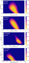 |
Fig. 2. Joint search of differential rotation and equatorial rotation period for HD 1835, HD 82443, and HD 206860. The panels illustrate the χr2 landscape over a grid of (Prot, eq, dΩ) pairs, with the 1σ and 3σ contours. The best values are obtained by fitting a 2D paraboloid around the minimum, while their error bars are estimated from the projection of the 1σ contour on the respective axis (Press et al. 1992). |
Our ZDI reconstruction of HD 1835 is shown in Fig. 3, exhibiting low-latitude, almost equatorial magnetic structures. The field has a predominantly poloidal component (91% of the total magnetic energy), of which 32%, 28%, and 37% is in the dipolar, quadrupolar and octupolar modes. The field is largely non-axisymmetric, since the axisymmetric component (that is, ℓ ≥ 1 and m = 0) accounts for 6% of the total energy. The reconstructed field shows similarities with the 2013 map of Rosén et al. (2016) and the 2017 map of Willamo et al. (2022), both in terms of dominant component and axisymmetry. Compared to Rosén et al. (2016) reconstruction, our map manifests an increased quadrupolar component at the expense of the dipolar component, indicating a higher complexity. Compared to Willamo et al. (2022), our ZDI reconstruction of the radial field features a more extended area covered by negative polarity.
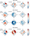 |
Fig. 3. Reconstructed large-scale magnetic field map of HD 1835, HD 43162, and HD 82443 in flattened polar view. From the left, the radial, azimuthal, and meridional components of the magnetic field vector are illustrated. The radial ticks are located at the rotational phases when the observations were collected (see Eq. (1)), while the concentric circles represent different stellar latitudes: –30 °, +30 °, and +60 ° (dashed lines), as well as the equator (solid line). |
The average magnetic field strength we recovered is 7 G, which is approximately half the value from previous reconstructions. This goes in the same direction as the decreased range of variability of the longitudinal field. For HD 1835, Egeland (2017) reported two superimposed activity cycles with two main periodicities of 7.8 yr and 20.8 yr. In a similar manner, Boro Saikia et al. (2018) estimated periodicities of 9.06 yr and 22 yr. Although there are three large-scale magnetic field maps reconstructed for this star, they are more recent than the temporal baseline of S-index values used by Egeland (2017) and Boro Saikia et al. (2018), which complicates the comparison of the field topology and the phase of the S-index cycle.
5.2. HD 28205 (V993 Tau)
HD 28205 is a G0.0 dwarf (Linsky et al. 2020) at a distance of 46.98 pc (Gaia Collaboration 2020). It is located in the Hyades cluster (Kraft 1965) and its age was estimated to be 630 Myr (Linsky et al. 2020), and its rotation period to 5.87 d (Pizzolato et al. 2003).
We measured logR′HK values between −4.453 and −4.424, with a median of −4.438 ± 0.009 (the median error is 0.036 in comparison). These values are about 0.06 dex larger than the average index given in Brown et al. (2022). The Hα index is stable around 0.313 ± 0.001, and the Ca II IRT varies between 0.843 and 0.849 with a median value of 0.848 ± 0.002.
The longitudinal field was measured to be between −2.9 and 0.8 G, with a median value of −1.0 ± 1.3 G (the median error bar is 1.7 G). The value is on the same order of magnitude as the unsigned, average longitudinal field reported by Brown et al. (2022). Since we only had five observations for this star, mostly clustered around rotational phase 0.0, we did not perform temporal analyses or ZDI.
5.3. HD 30495 (IX Eri)
HD 30495 is a G2.5 dwarf (Gray et al. 2006) at a distance of 13.24 pc (Gaia Collaboration 2020). It has an age of 400 Myr (Ramírez et al. 2012) and a rotation period of 11.36 d (Egeland et al. 2015).
We measured logR′HK values between −4.481 and −4.495, with a median of −4.490 ± 0.006 (the median error is 0.030 in comparison). These values are compatible with Boro Saikia et al. (2018) and Brown et al. (2022), but on the higher end of the range listed. This could be explained by the chromospheric activity cycle of the star, composed of two superimposed periodicities of 2 and 12 yr (Egeland et al. 2015; Brandenburg et al. 2017). More precisely, extrapolating the trend shown in Fig. 1 of Egeland et al. (2015), we note that the 2015 observations analysed by Brown et al. (2022) lie at a lower activity state than our 2018 observations. The Hα index we computed is constant around 0.323 ± 0.001, and the Ca II IRT is stable around 0.855 ± 0.001.
The longitudinal field was measured to be between 0.4 and 3.1 G, with a median value of 1.6 ± 1.1 G (the median error bar is 1.1 G). The range is compatible with the unsigned, average longitudinal field reported by Brown et al. (2022). Since we only have three observations for this star, we did not perform any temporal analyses or ZDI.
5.4. HD 43162 (V352 CMa)
HD 43162 A is a G6.5 dwarf (Linsky et al. 2020), and it is the primary component of a triple system at a distance of 16.69 pc (Chini et al. 2014; Gaia Collaboration 2020). It has an age of 320 Myr (Linsky et al. 2020) and a rotation period of 8.50 d (Marsden et al. 2014).
We measured logR′HK values between −4.398 and −4.315, with a median of −4.364 ± 0.023. While these values indicate a higher activity level than reported in Marsden et al. (2014) and Lehtinen et al. (2016) by about 0.06 dex, they are compatible with the measurements by Boro Saikia et al. (2018) and Brown et al. (2022). The Hα index varies between 0.336 and 0.342, with a median of 0.339 ± 0.002, and the Ca II IRT ranges between 0.891 and 0.919 with a median value of 0.903 ± 0.007. The longitudinal field was measured to be between −4.9 and 7.2 G, with a median value of 2.4 ± 3.3 G (the median error bar is 1.5 G). This range encompasses the value reported in Marsden et al. (2014) as well as the unsigned average in Brown et al. (2022).
We carried out a ZDI reconstructions for both epochs of HD 43162. The maps are shown in Fig. 3 and the model Stokes V profiles in Fig. D.1. In this case, reliable Stokes V models of the LSD profiles could only be obtained with an optimisation of veqsini based on χ2 minimisation. The idea is similar to the grid search used to find differential rotation (see Sect. 4); however, in this case, only a grid over veqsini was used, while all the other parameters were kept fixed. We obtained a value of 7 km s−1, which is lower than the value of 9.6 km s−1 estimated by Valenti & Fischer (2005), but consistent with previous measurements by Zejda et al. (2012). We then searched for the optimised values of rotation period and differential rotation jointly, but the results were inconclusive; hence, we performed ZDI reconstructions assuming solid body rotation. When searching for the optimised value of rotation period alone, we found a χ2 minimum at the expected rotation period of 8.5 d (Lehtinen et al. 2020) for both epochs; hence, we used this value for the ZDI maps.
For the 2019.01 epoch, we set a target χr2 to 1.7 from an initial value of 6.2. We found an average field strength of 11 G, with the topology being 64% poloidal and 36% toroidal. The dipolar mode dominates the poloidal component by storing 84% of the magnetic energy, while the quadrupolar and octupolar account for 11% and 4%, respectively. The axisymmetric component is 64%. For 2019.22, the target χr2 is 1.5, from an initial value of 11.2. The average field strength is 16 G, and the field configuration is predominantly toroidal (63%). The poloidal component is still largely dipolar (63%), but the quadrupolar and octupolar components increased to 26% and 8%.
No polarity reversal is seen between the two epochs. While we cannot exclude an evolution of the field on short timescales, the difference in dominant topology between the two epochs could also be due to the scarce phase coverage affecting the 2019.01 epoch. Furthermore, we observe that the Stokes V signatures are asymmetric: a larger positive lobe than the negative one (see Fig. D.1). The spurious polarisation signature in Stokes N is negligible compared to the Stokes V signature; hence, it does not affect its shape and symmetry. The asymmetry in Stokes V has been encountered before for solar-like stars such as ξ Boo A (Petit et al. 2005; Morgenthaler et al. 2012) as well as more massive stars such as θ Leo and ε UMa (Blazère et al. 2016). We note that this might be due to vertical gradients of photospheric velocity and magnetic field strength (López Ariste 2002). Interestingly, we only found this feature in the case of HD 43162.
5.5. HD 82443 (DX Leo)
HD 82443 is a G9.0 dwarf (Gray et al. 2003), and it is the primary of a binary system with an M6 dwarf (Lépine & Bongiorno 2007) at a distance of 18.07 pc (Gaia Collaboration 2020). It is a member of the Her-Lyr moving group (Gaidos 1998; Eisenbeiss et al. 2013), with an age of 250 Myr (Folsom et al. 2016; Linsky et al. 2020) and a rotation period of Prot = 5.377 d (Folsom et al. 2016).
We measured logR′HK values between −4.170 and −4.115, with a median of −4.147 ± 0.016 (the median error bar is 0.011). These values are 0.05 dex larger than the average values reported in Folsom et al. (2016), Boro Saikia et al. (2018), and Brown et al. (2022). The Hα index varies between 0.375 and 0.383, with a median of 0.380 ± 0.003, and the Ca II IRT ranges 0.974–0.995 with a median value of 0.986 ± 0.006. The values of both indices are ∼0.015 units higher than the values measured by (Folsom et al. 2016).
The longitudinal field was measured to be between −10.9 and 1.3 G, with a median value of −4.1 ± 8.4 G (the median error bar is 1.3 G). In comparison, Folsom et al. (2016) measured the longitudinal field to be between ±20 G, and Brown et al. (2022) obtained an average Bl of 11 G in absolute value.
We applied ZDI and fit the Stokes V time series down to χr2 = 2.2 from an initial value of 35.1, when assuming solid body rotation. We then searched for differential rotation and constrained Prot = 5.460 ± 0.026 d and dΩ = 0.114 ± 0.022 rad d−1 (see Fig. 2). We caution that measurements of the differential rotation with less than 15 observations across the stellar rotation may be biased due to rotational phase gaps (Petit et al. 2002). The rotation period is consistent with the value constrained with ZDI by Folsom et al. (2016) within 1σ. Our differential rotation rate is ∼2σ larger than the lower limit estimated from photometric light curves by Messina et al. (1999). Using Eq. (6), we estimated a rotation period at the pole of 6.070 ± 0.130 d. By assuming our Prot, dΩ pair, the target χr2 of the ZDI reconstruction was improved to 1.7.
The magnetic field topology is shown in Fig. 3 and the properties listed in Table 2. We obtained an average magnetic field strength of 23 G, which is consistent with the reconstruction of Folsom et al. (2016). The magnetic field topology is predominantly poloidal (64%), with 34%, 47%, and 9% of the magnetic energy stored in the dipolar, quadrupolar, and octupolar modes, respectively. The field is also non-axisymmetric (36%). In comparison, the reconstruction of Folsom et al. (2016) using 2013 data exhibits a predominantly dipolar (71%) and non-axisymmetric (8%) topology, indicating an increase in complexity with our recent observations. Considering the toroidal component specifically, the axisymmetric energy fraction increases from 38% in Folsom et al. (2016) to 92% in our reconstruction. This evolution occurred over a timescale of approximately 5 yr, which is similar on the same order of magnitude as the photometric activity cycle reported by Baliunas et al. (1995), Messina et al. (1999), Lehtinen et al. (2016). If we assume that the dynamo processes operating in the stellar interior are Sun-like, we could attribute the evolution of the axisymmetric-toroidal fraction to a correlated, equatorward distribution of starspots.
5.6. HD 114710 (β Com)
HD 114710 is a G0.0 dwarf (Keenan & McNeil 1989) at a distance of 9.19 pc (Gaia Collaboration 2020) and part of a visual binary system (Mason et al. 2001). It has an age of 1.60 Gyr (Ramírez et al. 2012) and a rotation period of Prot = 12.35 d (Wright et al. 2011).
We measured logR′HK values between −4.633 and −4.591, with a median of −4.609 ± 0.011 (the median error bar is comparable to the standard deviation). These values are compatible with the measurements reported by Boro Saikia et al. (2018) and Brown et al. (2022). The Hα index varies between 0.312 and 0.315, with a median of 0.313 ± 0.001, and the Ca II IRT ranges 0.793–0.813 with a median value of 0.798 ± 0.006. The longitudinal field was measured to be between −2.7 and 0.7 G, with a median value of −0.3 ± 1.0 G (where the median error bar is 0.5 G).
The Stokes V time series was fit down to χr2 = 1.6 from an initial value of 5.5 assuming solid body rotation, since the differential rotation search was inconclusive. The maps and the Stokes V fits are shown in Fig. 4 and Fig. D.1, respectively. We caution that the amplitude of the spurious polarisation signature in Stokes N is of the same order of magnitude as the Zeeman signature in Stokes V for this star, but the shape and amplitude of Stokes V seems to be unaffected by the presence (or absence) of the Stokes N signature (see also Sect. 2). The properties of the field topology are listed in Table 2. The magnetic field is predominantly poloidal (89%), with 60%, 25%, and 10% of the magnetic energy stored in the dipolar, quadrupolar, and octupolar modes, respectively. The field is also non-axisymmetric (31% in the axisymmetric components) and exhibits an average field strength of 1.3 G.
 |
Fig. 4. Reconstructed large-scale magnetic field map of HD 114710, HD 189733, and HD 206860 for the two epochs. The format is the same as Fig. 3. |
5.7. HD 149026 (HIP 808308)
HD 149026 is a G0.0 dwarf (Sato et al. 2005) at a distance of 76.21 pc (Gaia Collaboration 2020). Its age was estimated to be 2.78 Gyr (Ramírez et al. 2012). This star is known to host a Saturn-like planet with a mass of 0.38 MJup on a 2.87 d orbit (Sato et al. 2005; Bonomo et al. 2017). While there is no measurement of the rotation period for this star in the literature, we estimated a value of 12.3 ± 1.2 d using the radius and the projected equatorial velocity (see Table 1).
From the three Narval observations, we measured logR′HK values between −4.903 and −4.886, with a median of −4.900 ± 0.010. The value is consistent with Boro Saikia et al. (2018) and Brown et al. (2022). The Hα index is stable at 0.308, and the Ca II IRT ranges 0.763–0.774 with a median value of 0.768 ± 0.004.
Overall, this star is the least active of our sample. We did not detect any evident Zeeman signatures from the circularly polarised spectra of this star, but only one observation led to a marginal detection with a longitudinal magnetic field of 3.4 ± 2.0 G. From observations with non-detections, we can still use Eq. (5) to compute a Bl value with error bar to determine the upper limits. The two non-detection observations led to 0.35 ± 2.1 G and 2.2 ± 2.2 G; thus, we placed a 3σ upper limit of 6 G to the longitudinal field detection (see Table C.1).
5.8. HD 189733 (V452 Vul)
HD 189733 is a K2.0 dwarf (Gray et al. 2003) at a distance of 19.78 pc (Gaia Collaboration 2020), and it is part of a visual binary system (Mason et al. 2001). The age is 400 Myr (Ramírez et al. 2012), while the rotation period is 11.94 d (Fares et al. 2010). The star hosts a hot Jupiter on a 2.22 d orbit (Bouchy et al. 2005).
We measured logR′HK values between −4.485 and −4.449, with a median of −4.473 ± 0.011 (the median error bar is 0.026). Our range is compatible with the value computed by Brown et al. (2022) and 0.05 dex larger than that reported by Boro Saikia et al. (2018). The Hα index varies between 0.362 and 0.364, with a median of 0.363 ± 0.001, and the Ca II IRT ranges 0.862–0.880 with a median value of 0.867 ± 0.005.
The longitudinal field was measured to be between −4.3 and 1.8 G, with a median value of −0.3 ± 2.0 G (the median error bar is 1.1 G). In comparison, Brown et al. (2022) measured an average Bl of 4.5 G in absolute value.
We applied ZDI and fit the Stokes V time series down to χr2 = 1.8 from an initial value of 15.1, assuming solid body rotation. The maps are shown in Fig. 4 and the Stokes V models in Fig. D.1. The search for differential rotation was inconclusive, owing to both a sparse time series and the poor phase coverage (mostly between 0.0 and 0.5). Thus, we attempted to carry out ZDI reconstructions with values of differential rotation rates obtained from previous ZDI reconstructions: dΩ = 0.146 ± 0.049 rad d−1 (Fares et al. 2010) and dΩ = 0.110 ± 0.050 rad d−1 from Fares et al. (2017). In both cases, the value of the target χr2 was improved to ∼1.7. Compared to the ZDI map obtained assuming solid body rotation, the maps including dΩ differ by less than 0.5 G in average field strength, less than 3% in poloidal energy fraction, and less than 0.5% for the axisymmetric energy fraction. The same was found for the dipolar and octupolar components, while the quadrupolar energy fraction decreased from 30 to 20%, implying a simpler magnetic field configuration when differential rotation was accounted for. We decided to fix dΩ = 0.110 rad d−1 from Fares et al. (2017) since it was derived using the largest number of observations and for a data set in 2013, which is closest in time to our observations.
The properties of the magnetic topology are listed in Table 2. The field has an average field strength of 18 G, and it has 52% of the magnetic energy in the poloidal component, which is predominantly dipolar (68%). The quadrupolar and octupolar components account for 16% and 8% of the energy, while the axisymmetric component is 44%. Even though our map is reconstructed without an ideal phase coverage of the stellar rotation, our results are consistent with the previous reconstructions of Moutou et al. (2007), Fares et al. (2010, 2017), with an equatorial magnetic spot of positive polarity in the radial component and an azimuthal component dominated by a negative polarity (see Fig. 3 in Fares et al. 2017). These authors studied the evolution of the magnetic topology of HD 189733 from a nine-year spectropolarimetric monitoring. In addition, although a magnetic cycle could not be constrained, they corroborated the fast evolution of the topology over a few stellar rotations. This was manifested mainly in the variations in axisymmetry and poloidal-to-toroidal energy fraction, but the toroidal component was always the dominant one.
5.9. HD 190406 (GJ 779)
HD 190406 is a G0.0 dwarf (Gray et al. 2006) at a distance of 17.77 pc (Gaia Collaboration 2020), and it is part of a visual binary system (Mason et al. 2001). The estimated age is 1.70 Gyr (Ramírez et al. 2012) and the rotation period is Prot = 13.94 d (Wright et al. 2011).
We measured logR′HK values between −4.719 and −4.663, with a median of −4.697 ± 0.019, which is consistent with the values reported by Boro Saikia et al. (2018) and Brown et al. (2022). The Hα index varies between 0.312 and 0.314, and the Ca II IRT ranges 0.789–0.800 with a median value of 0.795 ± 0.003. We did not detect any Stokes V signatures in the eight Narval observations of this star. The average longitudinal field is 0.9 G and the average uncertainty is 1.0 G; thus, we set a 3σ upper limit of 3 G (see Table C.1).
5.10. HD 206860 (HN Peg)
HD 206860 is a G0.0 dwarf (Gray et al. 2001) at a distance of 18.13 pc (Gaia Collaboration 2020), and it is part of a visual binary system (Mason et al. 2001). It is a member of the Her-Lyr moving group (Eisenbeiss et al. 2013), with an age of 200 Myr (Güdel 2007; Ramírez et al. 2012) and a rotation period of Prot = 4.55 d (Boro Saikia et al. 2015). The star hosts a 16-MJup planet at a distance of 773 au (Luhman et al. 2007).
We measured logR′HK values between −4.356 and −4.294, with a median of −4.334 ± 0.017 (the median error bar is similar to the standard deviation). These values are at most 0.07 dex larger than the values reported in Marsden et al. (2014), Boro Saikia et al. (2015), Boro Saikia et al. (2018), and Brown et al. (2022). The Hα index varies between 0.326 and 0.331, with a median of 0.327 ± 0.001, which is 0.012 and 0.005 units larger than the values of Marsden et al. (2014) and Boro Saikia et al. (2015), respectively. The Ca II IRT ranges 0.895–0.929 with a median value of 0.910 ± 0.008, which is comparable to the range of values from both Marsden et al. (2014) and Boro Saikia et al. (2015).
The longitudinal field was measured to be between 2.5 and 10.5 G, with a median value of 5.2 ± 3.4 G (the median error bar is 1.5 G). In comparison, Boro Saikia et al. (2015) measured longitudinal field values between ±14 G, and Brown et al. (2022) obtained an average Bl of 6.4 G in absolute value terms.
The ZDI reconstructions were performed for 2018 and 2019 epochs of HD 206860. The maps are shown in Fig. 4 and the Stokes V models in Fig. D.1. Assuming solid body rotation, the target χr2 is 2.0 and 1.6 starting from 11.7 and 13.0 for the 2018 and 2019 epochs, respectively. We then constrained differential rotation via χ2 minimisation (see Fig. 2). In 2018, we obtained Prot = 4.723 ± 0.003 d and dΩ = 0.109 ± 0.004 rad d−1 (implying a rotation period at the pole of 5.145 ± 0.017 d), while in 2019 we obtained Prot = 4.650 ± 0.017 d and dΩ = 0.051 ± 0.042 rad d−1 (corresponding to 4.832 ± 0.157 d at the pole). Using these values, the target χr2 was improved to 1.3 and 1.1 for the two epochs. The values of dΩ differ by roughly a factor of two, but they are reasonably consistent within uncertainties. The error bar on the differential rotation rate extracted from the 2019 epoch is larger owing to the incomplete phase coverage of the observations used in the analysis.
We note that the differential rotation rates we constrained for 2018 and 2019 are a factor of 2 and 4 smaller, respectively, than those measured by Boro Saikia et al. (2015). If we were to perform the ZDI reconstruction using dΩ = 0.22 rad d−1 from Boro Saikia et al. (2015), the χr2 improvement would not be as substantial (of about 0.1–0.2) as when using our derived values. This may suggest an evolution of the differential shear at the surface of the star, which was also recorded for other stars (AB Dor, LQ Hya, and HR 1099; Donati et al. 2003), and for the Sun in correlation with the magnetic cycle (Poljančić Beljan et al. 2022).
The properties of the field topology are listed in Table 2. In 2018, the magnetic field is predominantly poloidal (86%), with 47%, 17%, and 14% of the magnetic energy stored in the dipolar, quadrupolar, and octupolar modes, respectively, while the axisymmetric component accounts for 65% of the total magnetic energy. The situation is similar for 2019, the main difference being the decrease in the poloidal component to 69% and the corresponding increase in the toroidal component. The poloidal component also becomes more dipolar (60%). In terms of average magnetic field strength, the 2018 epoch featured a value of 21 G, while in 2019 it decreased to 16 G.
In general, the maps of HD 206860 are consistent with both the ZDI reconstructions done by Rosén et al. (2016), with Narval data between 2007–2011 and HARPS-Pol in 2013, and by Boro Saikia et al. (2015), with the Narval 2007–2011 time series. Indeed, they also feature a primarily poloidal, dipolar, and axisymmetric configuration, with the positive polarity predominantly located in the northern hemisphere. The maps also share similarities in terms of complexity, with magnetic patches extending down to low latitudes. More specifically, our reconstructions from 2018 and 2019 resemble the previous ZDI maps based on the 2009 data.
5.11. HD 219828 (HIP 115100)
HD 219828 is a G0.0 dwarf (Moore & Paddock 1950) at a distance of 72.56 pc (Gaia Collaboration 2020). The estimated age is 6.08 Gyr (Ramírez et al. 2012) and the rotation period is Prot = 28.70 d (Santos et al. 2016). This is the most distant, oldest, and slowest rotator in our sample. The star hosts a hot Neptune (mass of 0.06 MJup) and a long-period planet (mass of 15 MJup) at a distance of 0.05 and 5.8 au, respectively (Santos et al. 2016).
We measured logR′HK values between −5.000 and −4.966, with a median of −4.986 ± 0.011, which is 0.1 dex lower than what was reported by Boro Saikia et al. (2018). The Hα index varies between 0.316 and 0.318, and the Ca II IRT ranges 0.747–0.783 with a median value of 0.758 ± 0.010. We did not clearly detect Stokes V signatures in the ten Narval observations of this star. For one of them, there is a marginal detection and its associated longitudinal magnetic field is 3.6 ± 2.0 G. The average longitudinal field is 1 G and the average uncertainty is 1.8 G, so we set a 3σ upper limit of 5 G.
6. Activity trends
As summarised in Table 1, the stars in our sample have ages between 0.2 and 6.1 Gyr, while the rotation period ranges between 4.6 and 28.7 d. Although the main purpose of this work is to provide magnetic field maps for modelling the stellar wind and environment in a subsequent paper, it is interesting to contextualise our measurements of activity indicators, longitudinal field, and magnetic field properties with previous studies. In particular, we discuss the trends with respect to stellar age and rotation period below.
Studies of activity indices around cool stars on the main sequence by Pace (2013), Marsden et al. (2014), and Brown et al. (2022) showed a decrease in stellar activity with increasing stellar age and rotation period. We noted a consistent behaviour (see Fig. 5 and Table C.1), where larger average values of activity indicators and longitudinal field towards younger and faster rotating stars. Quantitatively, we observe for example that our median longitudinal field decreases from 5 G to less than 1 G over from 0.1 to 4 Gyr (or from 5 d to 15 d rotation period) and our logR′HK decreases from −4.2 to −5.0.
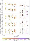 |
Fig. 5. Trends of activity indices and reconstructed magnetic field geometry with age. From the top: logR′HK, average magnetic field strength, poloidal fraction of the total energy, dipolar fraction of the poloidal energy, and axisymmetric fraction of the total energy. Properties measured for the same star but at different epochs are connected by a solid line. Our measurements are represented by ‘X’ and measurements by Folsom et al. (2016, 2018, and references therein) and Bellotti et al. (2025) are indicated with circles. The solar values from the work of Egeland (2017) and Vidotto et al. (2018) are also included. |
Turning to the large-scale magnetic field geometry, Vidotto et al. (2014b), Folsom et al. (2016, 2018), Rosén et al. (2016) reported trends across different ages and rotation periods for Sun-like stars similar to those examined in this work. They reported a clear trend of decreasing average magnetic field with increasing age and rotation period, which we consistently observed for our stars as well. The average field strength of our six stars exhibits a decrease from 25 to 10 G between 0.2 and 0.4 Gyr. The oldest star in this sub-sample (at 1.6 Gyr) has an average magnetic field strength of 1 G. We show this trend in Fig. 5, where we complement our measurements with those of Petit et al. (2008), Folsom et al. (2016, 2018), and Bellotti et al. (2025).
Figure 5 also shows the variation with age and rotation period of the magnetic energy fraction in the poloidal, dipolar, and axisymmetric components. The addition of our measurements did not reveal clear trends in dipolar nor axisymmetric energy fraction, as already reported in Folsom et al. (2018). For the poloidal energy fraction, we expect the magnetic field of slow rotators and old stars to have a predominantly poloidal geometry, while faster-rotating and younger stars to have mixed geometries (Petit et al. 2008; Folsom et al. 2016). Our measurements are consistent with these expectations.
Overall, although the age estimate is not used in a ZDI reconstruction, inhomogeneous or inaccurate age measurements can increase scatter. Moreover, the search of these trends is complicated by temporal variations in the magnetic field in the form of intrinsic variability (short-term) or magnetic cycles (long-term), as revealed also for other Sun-like stars by spectropolarimetry (e.g. Boro Saikia et al. 2016; Mengel et al. 2016; Fares et al. 2017; Jeffers et al. 2022; Bellotti et al. 2025). For two of the stars examined here, HD 43162 and HD 206860, we reconstructed two maps corresponding to two distinct observational epochs. The magnetic properties reconstructed with ZDI are different at these epochs, which increases the scatter as illustrated in Fig. 5. A more thorough search for trends of the magnetic geometry over age and characterisation of this scatter would require multiple ZDI maps for the same star over different years to include such a temporal variability (Jeffers et al. 2023).
7. Conclusions
In this study, we analysed the spectropolarimetric time series of eleven Sun-like stars collected with Narval between 2018 and 2019. Our aim has been to characterise the magnetic properties of these stars for subsequent modelling of their stellar environments, which is topical in light of space-based missions dedicated to planetary atmospheric characterisation (e.g. JWST currently and Ariel in the future), as well as for direct imaging (e.g. LIFE; Quanz et al. 2018, 2022 and the Habitable World Observatory; National Academies of Sciences and Engineering, Medicine 2021). Indeed, knowledge of the stellar magnetic environment that exoplanets are embedded in feeds back to, for instance, the interpretation of atmospheric signatures due to star-planet interactions (e.g. Carolan et al. 2021; Gupta et al. 2023), as well as habitability assessments (e.g. Vidotto et al. 2013; Lingam & Loeb 2019; Van Looveren et al. 2024).
The stellar ages and rotation periods of our stars span different regions of the parameter space, from 0.2 to 6.1 Gyr and from 4.6 to 28.7 d, respectively, allowing us to sample stellar activity and magnetic field properties at different stages on the main sequence. As a first-order characterisation of the stars’ magnetic activity, we computed chromospheric activity indices such as logR′HK, Hα, and the Ca II infrared triplet from unpolarised spectra as well as the longitudinal magnetic field Bl from circularly polarised spectra. Overall, we noted trends expected from previous work: in particular, stellar activity decreasing with increasing age and rotation period (e.g. Marsden et al. 2014; Brown et al. 2022).
For the six stars with a detectable circular polarisation signature and large number of observations, we reconstructed the large-scale magnetic field configuration via ZDI. This was the first magnetic field reconstruction for two stars: HD 43162 and HD 114710. The properties of the large-scale magnetic field are in good agreement in terms of field strength and complexity with stars of similar properties. We found average magnetic field strengths ranging from 1 to 25 G, where the lowest values belong to old or slow rotating stars, consistently with what is expected for this stellar parameter space (see e.g. Rosén et al. 2015; Folsom et al. 2016, 2018). Most stars exhibit complex magnetic fields that are predominantly poloidal and with a significant (> 10%) toroidal component and with distinct degrees of axisymmetry.
In agreement with See et al. (2015) and Folsom et al. (2018), we found that the poloidal-dominated topologies have various levels of axisymmetry, whereas the toroidal-dominated topologies are mostly axisymmetric. We also observed a decreasing trend of the average field strength with increasing age and rotation period. We did not record evident trends among the magnetic field properties, such as the poloidal fraction or axisymmetric fraction with respect to stellar age and rotation period, which could be due to temporal variations in the field topology, namely, in the magnetic cycles.
Our results stress the importance of spectropolarimetric studies to investigate the magnetic field properties of exoplanet-hosting stars, given the variety of properties of the large-scale magnetic field for Sun-like stars over time. This likely translates into a variety of stellar wind properties and offers a range of diverse magnetic environments in which exoplanets could be embedded. Ultimately, this study comprises a systematic attempt to characterise the evolution of environmental conditions and habitability of exoplanets from the perspective of stellar magnetism.
Data availability
All analysed spectropolarimetric observations collected with Narval are available in Polarbase. They can be found at https://www.polarbase.ovgso.fr/
The data is available at https://www.polarbase.ovgso.fr/
Available at https://github.com/folsomcp/LSDpy
Acknowledgments
S.B. acknowledges funding by the Dutch Research Council (NWO) under the project “Exo-space weather and contemporaneous signatures of star-planet interactions” (with project number OCENW.M.22.215 of the research programme “Open Competition Domain Science- M”). S.B. also acknowledges funding from the SCI-S department of the European Space Agency (ESA), under the Science Faculty Research fund E/0429-03. S.B.S. acknowledges funding from the Austrian Science Fund (FWF) Lise Meitner project M2829-N. C.P.F. acknowledges funding from the European Union’s Horizon Europe research and innovation program under grant agreement No. 101079231 (EXOHOST), and from the United Kingdom Research and Innovation Horizon Europe Guarantee Scheme (grant No. 10051045). This work used the Dutch national e-infrastructure with the support of the SURF Cooperative using grant nos. EINF-2218 and EINF-5173. Based on observations obtained at the Canada-France-Hawaii Telescope (CFHT) which is operated by the National Research Council of Canada, the Institut National des Sciences de l’Univers of the Centre National de la Recherche Scientique of France, and the University of Hawaii. This work has made use of the VALD database, operated at Uppsala University, the Institute of Astronomy RAS in Moscow, and the University of Vienna; Astropy, a community-developed core Python package for Astronomy (Astropy Collaboration 2013, 2018); NumPy (van der Walt et al. 2011); Matplotlib: Visualization with Python (Hunter 2007); SciPy (Virtanen et al. 2020) and PyAstronomy (Czesla et al. 2019).
References
- Airapetian, V. S., & Usmanov, A. V. 2016, ApJ, 817, L24 [Google Scholar]
- Airapetian, V. S., Barnes, R., Cohen, O., et al. 2020, Int. J. Astrobiol., 19, 136 [NASA ADS] [CrossRef] [Google Scholar]
- Allan, A., & Vidotto, A. A. 2019, MNRAS, 490, 3760 [Google Scholar]
- Alvarado-Gómez, J. D., Hussain, G. A. J., Grunhut, J., et al. 2015, A&A, 582, A38 [NASA ADS] [CrossRef] [EDP Sciences] [Google Scholar]
- Alvarado-Gómez, J. D., Hussain, G. A. J., Drake, J. J., et al. 2018, MNRAS, 473, 4326 [CrossRef] [Google Scholar]
- Alvarado-Gómez, J. D., Cohen, O., Drake, J. J., et al. 2022, ApJ, 928, 147 [CrossRef] [Google Scholar]
- Astropy Collaboration (Robitaille, T. P., et al.) 2013, A&A, 558, A33 [NASA ADS] [CrossRef] [EDP Sciences] [Google Scholar]
- Astropy Collaboration (Price-Whelan, A. M., et al.) 2018, AJ, 156, 123 [Google Scholar]
- Bagnulo, S., Landolfi, M., Landstreet, J. D., et al. 2009, PASP, 121, 993 [Google Scholar]
- Baliunas, S. L., Donahue, R. A., Soon, W. H., et al. 1995, ApJ, 438, 269 [Google Scholar]
- Bellotti, S., Petit, P., Morin, J., et al. 2022, A&A, 657, A107 [NASA ADS] [CrossRef] [EDP Sciences] [Google Scholar]
- Bellotti, S., Fares, R., Vidotto, A. A., et al. 2023, A&A, 676, A139 [NASA ADS] [CrossRef] [EDP Sciences] [Google Scholar]
- Bellotti, S., Petit, P., Jeffers, S. V., et al. 2025, A&A, 693, A269 [NASA ADS] [CrossRef] [EDP Sciences] [Google Scholar]
- Blazère, A., Petit, P., Lignières, F., et al. 2016, A&A, 586, A97 [NASA ADS] [CrossRef] [EDP Sciences] [Google Scholar]
- Bonomo, A. S., Desidera, S., Benatti, S., et al. 2017, A&A, 602, A107 [NASA ADS] [CrossRef] [EDP Sciences] [Google Scholar]
- Boro Saikia, S., Jeffers, S. V., Petit, P., et al. 2015, A&A, 573, A17 [NASA ADS] [CrossRef] [EDP Sciences] [Google Scholar]
- Boro Saikia, S., Jeffers, S. V., Morin, J., et al. 2016, A&A, 594, A29 [NASA ADS] [CrossRef] [EDP Sciences] [Google Scholar]
- Boro Saikia, S., Lueftinger, T., Jeffers, S. V., et al. 2018, A&A, 620, L11 [NASA ADS] [CrossRef] [EDP Sciences] [Google Scholar]
- Boro Saikia, S., Jin, M., Johnstone, C. P., et al. 2020, A&A, 635, A178 [NASA ADS] [CrossRef] [EDP Sciences] [Google Scholar]
- Bouchy, F., Udry, S., Mayor, M., et al. 2005, A&A, 444, L15 [EDP Sciences] [Google Scholar]
- Brandenburg, A., Mathur, S., & Metcalfe, T. S. 2017, ApJ, 845, 79 [NASA ADS] [CrossRef] [Google Scholar]
- Brown, E. L., Jeffers, S. V., Marsden, S. C., et al. 2022, MNRAS, 514, 4300 [CrossRef] [Google Scholar]
- Busà, I., Aznar Cuadrado, R., Terranegra, L., Andretta, V., & Gomez, M. T. 2007, A&A, 466, 1089 [NASA ADS] [CrossRef] [EDP Sciences] [Google Scholar]
- Carolan, S., Vidotto, A. A., Villarreal D’Angelo, C., & Hazra, G. 2021, MNRAS, 500, 3382 [Google Scholar]
- Cecchi-Pestellini, C., Ciaravella, A., & Micela, G. 2006, A&A, 458, L13 [NASA ADS] [CrossRef] [EDP Sciences] [Google Scholar]
- Chini, R., Fuhrmann, K., Barr, A., et al. 2014, MNRAS, 437, 879 [CrossRef] [Google Scholar]
- Claret, A., & Bloemen, S. 2011, A&A, 529, A75 [NASA ADS] [CrossRef] [EDP Sciences] [Google Scholar]
- Cockell, C. S., Bush, T., Bryce, C., et al. 2016, Astrobiology, 16, 89 [NASA ADS] [CrossRef] [Google Scholar]
- Czesla, S., Schröter, S., Schneider, C. P., et al. 2019, Astrophysics Source Code Library [record ascl:1906.010] [Google Scholar]
- Donati, J. F. 2003, in Solar Polarization, eds. J. Trujillo-Bueno, & J. Sanchez Almeida, Astronomical Society of the Pacific Conference Series, 307, 41 [Google Scholar]
- Donati, J. F., & Brown, S. F. 1997, A&A, 326, 1135 [Google Scholar]
- Donati, J. F., & Collier Cameron, A. 1997, MNRAS, 291, 1 [NASA ADS] [CrossRef] [Google Scholar]
- Donati, J. F., & Landstreet, J. D. 2009, Annu. Rev. Astron. Astrophys., 47, 333 [Google Scholar]
- Donati, J. F., Semel, M., Carter, B. D., Rees, D. E., & Collier Cameron, A. 1997, MNRAS, 291, 658 [Google Scholar]
- Donati, J. F., Mengel, M., Carter, B. D., et al. 2000, MNRAS, 316, 699 [Google Scholar]
- Donati, J. F., Collier Cameron, A., & Petit, P. 2003, MNRAS, 345, 1187 [NASA ADS] [CrossRef] [Google Scholar]
- Donati, J. F., Morin, J., Petit, P., et al. 2008, MNRAS, 390, 545 [Google Scholar]
- Ducati, J. R. 2002, CDS/ADC Collection of Electronic Catalogues, 2237 [Google Scholar]
- Egeland, R. 2017, Ph.D. Thesis, Montana State University, Bozeman [Google Scholar]
- Egeland, R., Metcalfe, T. S., Hall, J. C., & Henry, G. W. 2015, ApJ, 812, 12 [NASA ADS] [CrossRef] [Google Scholar]
- Eisenbeiss, T., Ammler-von Eiff, M., Roell, T., et al. 2013, A&A, 556, A53 [NASA ADS] [CrossRef] [EDP Sciences] [Google Scholar]
- Evensberget, D., Carter, B. D., Marsden, S. C., Brookshaw, L., & Folsom, C. P. 2021, MNRAS, 506, 2309 [NASA ADS] [CrossRef] [Google Scholar]
- Evensberget, D., Carter, B. D., Marsden, S. C., et al. 2022, MNRAS, 510, 5226 [NASA ADS] [CrossRef] [Google Scholar]
- Evensberget, D., Marsden, S. C., Carter, B. D., et al. 2023, MNRAS, 524, 2042 [CrossRef] [Google Scholar]
- Fares, R., Donati, J. F., Moutou, C., et al. 2009, MNRAS, 398, 1383 [NASA ADS] [CrossRef] [Google Scholar]
- Fares, R., Donati, J. F., Moutou, C., et al. 2010, MNRAS, 406, 409 [NASA ADS] [CrossRef] [Google Scholar]
- Fares, R., Bourrier, V., Vidotto, A. A., et al. 2017, MNRAS, 471, 1246 [Google Scholar]
- Folsom, C. P., Petit, P., Bouvier, J., et al. 2016, MNRAS, 457, 580 [Google Scholar]
- Folsom, C. P., Bouvier, J., Petit, P., et al. 2018, MNRAS, 474, 4956 [NASA ADS] [CrossRef] [Google Scholar]
- Folsom, C. P., Ó Fionnagáin, D., Fossati, L., et al. 2020, A&A, 633, A48 [NASA ADS] [CrossRef] [EDP Sciences] [Google Scholar]
- Folsom, C. P., Erba, C., Petit, V., et al. 2025, arXiv e-prints [arXiv:2505.18476] [Google Scholar]
- Gaia Collaboration. 2020, VizieR Online Data Catalog: I/350 [Google Scholar]
- Gaidos, E. J. 1998, PASP, 110, 1259 [NASA ADS] [CrossRef] [Google Scholar]
- Gizis, J. E., Reid, I. N., & Hawley, S. L. 2002, AJ, 123, 3356 [Google Scholar]
- Gray, D. F., & Baliunas, S. L. 1997, ApJ, 475, 303 [Google Scholar]
- Gray, R. O., Napier, M. G., & Winkler, L. I. 2001, AJ, 121, 2148 [Google Scholar]
- Gray, R. O., Corbally, C. J., Garrison, R. F., McFadden, M. T., & Robinson, P. E. 2003, AJ, 126, 2048 [Google Scholar]
- Gray, R. O., Corbally, C. J., Garrison, R. F., et al. 2006, AJ, 132, 161 [Google Scholar]
- Güdel, M. 2007, Liv. Rev. Sol. Phys., 4, 3 [Google Scholar]
- Guinan, E. F., Ribas, I., & Harper, G. M. 2003, ApJ, 594, 561 [Google Scholar]
- Gupta, S., Basak, A., & Nandy, D. 2023, ApJ, 953, 70 [Google Scholar]
- Høg, E., Fabricius, C., Makarov, V. V., et al. 2000, A&A, 355, L27 [Google Scholar]
- Hunter, J. D. 2007, Comput. Sci. Eng., 9, 90 [NASA ADS] [CrossRef] [Google Scholar]
- Hussain, G. A. J., Collier Cameron, A., Jardine, M. M., et al. 2009, MNRAS, 398, 189 [Google Scholar]
- Jeffers, S. V., Boro Saikia, S., Barnes, J. R., et al. 2017, MNRAS, 471, L96 [NASA ADS] [Google Scholar]
- Jeffers, S. V., Cameron, R. H., Marsden, S. C., et al. 2022, A&A, 661, A152 [NASA ADS] [CrossRef] [EDP Sciences] [Google Scholar]
- Jeffers, S. V., Kiefer, R., & Metcalfe, T. S. 2023, Space Sci. Rev., 219, 54 [CrossRef] [Google Scholar]
- Johnstone, C. P., Güdel, M., Lüftinger, T., Toth, G., & Brott, I. 2015a, A&A, 577, A27 [NASA ADS] [CrossRef] [EDP Sciences] [Google Scholar]
- Johnstone, C. P., Güdel, M., Brott, I., & Lüftinger, T. 2015b, A&A, 577, A28 [NASA ADS] [CrossRef] [EDP Sciences] [Google Scholar]
- Johnstone, C. P., Bartel, M., & Güdel, M. 2021, A&A, 649, A96 [EDP Sciences] [Google Scholar]
- Joner, M. D., Taylor, B. J., Laney, C. D., & van Wyk, F. 2006, AJ, 132, 111 [Google Scholar]
- Keenan, P. C., & McNeil, R. C. 1989, ApJS, 71, 245 [Google Scholar]
- Ketzer, L., & Poppenhaeger, K. 2023, MNRAS, 518, 1683 [Google Scholar]
- Kochukhov, O., Makaganiuk, V., & Piskunov, N. 2010, A&A, 524, A5 [NASA ADS] [CrossRef] [EDP Sciences] [Google Scholar]
- Kochukhov, O., Hackman, T., Lehtinen, J. J., & Wehrhahn, A. 2020, A&A, 635, A142 [NASA ADS] [CrossRef] [EDP Sciences] [Google Scholar]
- Koen, C., Kilkenny, D., van Wyk, F., & Marang, F. 2010, MNRAS, 403, 1949 [Google Scholar]
- Kraft, R. P. 1965, ApJ, 142, 681 [Google Scholar]
- Kulikov, Y. N., Lammer, H., Lichtenegger, H. I. M., et al. 2007, Space Sci. Rev., 129, 207 [NASA ADS] [CrossRef] [Google Scholar]
- Lammer, H., Selsis, F., Ribas, I., et al. 2003, ApJ, 598, L121 [Google Scholar]
- Lammer, H., Güdel, M., Kulikov, Y., et al. 2012, Earth Planets Space, 64, 179 [NASA ADS] [CrossRef] [Google Scholar]
- Landi Degl’Innocenti, E. 1992, in Magnetic field measurements, eds. F. Sanchez, M. Collados, & M. Vazquez, 71 [Google Scholar]
- Landstreet, J. D. 2009, in Observing and Modelling Stellar Magnetic Fields 1. Basic Physics and Simple Models, eds. C. Neiner, & J. P. Zahn, EAS Publications Series, 39, 1 [Google Scholar]
- Lehmann, L. T., & Donati, J. F. 2022, MNRAS, 514, 2333 [CrossRef] [Google Scholar]
- Lehtinen, J., Jetsu, L., Hackman, T., Kajatkari, P., & Henry, G. W. 2016, A&A, 588, A38 [NASA ADS] [CrossRef] [EDP Sciences] [Google Scholar]
- Lehtinen, J. J., Spada, F., Käpylä, M. J., Olspert, N., & Käpylä, P. J. 2020, Nat. Astron., 4, 658 [Google Scholar]
- Lépine, S., & Bongiorno, B. 2007, AJ, 133, 889 [Google Scholar]
- Lingam, M., & Loeb, A. 2019, Int. J. Astrobiol., 18, 527 [NASA ADS] [CrossRef] [Google Scholar]
- Linsky, J. L., Wood, B. E., Youngblood, A., et al. 2020, ApJ, 902, 3 [NASA ADS] [CrossRef] [Google Scholar]
- Locci, D., Cecchi-Pestellini, C., & Micela, G. 2019, A&A, 624, A101 [NASA ADS] [CrossRef] [EDP Sciences] [Google Scholar]
- López Ariste, A. 2002, ApJ, 564, 379 [Google Scholar]
- Luhman, K. L., Patten, B. M., Marengo, M., et al. 2007, ApJ, 654, 570 [NASA ADS] [CrossRef] [Google Scholar]
- Marsden, S. C., Petit, P., Jeffers, S. V., et al. 2014, MNRAS, 444, 3517 [Google Scholar]
- Mason, B. D., Wycoff, G. L., Hartkopf, W. I., Douglass, G. G., & Worley, C. E. 2001, AJ, 122, 3466 [Google Scholar]
- Mathias, P., Aurière, M., López Ariste, A., et al. 2018, A&A, 615, A116 [NASA ADS] [CrossRef] [EDP Sciences] [Google Scholar]
- Mengel, M. W., Fares, R., Marsden, S. C., et al. 2016, MNRAS, 459, 4325 [NASA ADS] [CrossRef] [Google Scholar]
- Messina, S., Guinan, E. F., Lanza, A. F., & Ambruster, C. 1999, A&A, 347, 249 [NASA ADS] [Google Scholar]
- Middelkoop, F. 1982, A&A, 107, 31 [NASA ADS] [Google Scholar]
- Montes, D., López-Santiago, J., Gálvez, M. C., et al. 2001, MNRAS, 328, 45 [NASA ADS] [CrossRef] [Google Scholar]
- Moore, J. H., & Paddock, G. F. 1950, ApJ, 112, 48 [Google Scholar]
- Morgenthaler, A., Petit, P., Saar, S., et al. 2012, A&A, 540, A138 [NASA ADS] [CrossRef] [EDP Sciences] [Google Scholar]
- Moutou, C., Donati, J. F., Savalle, R., et al. 2007, A&A, 473, 651 [NASA ADS] [CrossRef] [EDP Sciences] [Google Scholar]
- Murray-Clay, R. A., Chiang, E. I., & Murray, N. 2009, ApJ, 693, 23 [Google Scholar]
- National Academies of Sciences and Engineering, Medicine. 2021, Pathways to Discovery in Astronomy and Astrophysics for the 2020s (Washington, DC: The National Academies Press) [Google Scholar]
- Nicholson, B. A., Vidotto, A. A., Mengel, M., et al. 2016, MNRAS, 459, 1907 [CrossRef] [Google Scholar]
- Noyes, R. W., Hartmann, L. W., Baliunas, S. L., Duncan, D. K., & Vaughan, A. H. 1984, ApJ, 279, 763 [Google Scholar]
- Owen, J. E., & Jackson, A. P. 2012, MNRAS, 425, 2931 [Google Scholar]
- Pace, G. 2013, A&A, 551, L8 [NASA ADS] [CrossRef] [EDP Sciences] [Google Scholar]
- Paegert, M., Stassun, K. G., Collins, K. A., et al. 2021, arXiv e-prints [arXiv:2108.04778] [Google Scholar]
- Penz, T., & Micela, G. 2008, A&A, 479, 579 [NASA ADS] [CrossRef] [EDP Sciences] [Google Scholar]
- Petit, P., Donati, J. F., & Collier Cameron, A. 2002, MNRAS, 334, 374 [NASA ADS] [CrossRef] [Google Scholar]
- Petit, P., Donati, J. F., Aurière, M., et al. 2005, MNRAS, 361, 837 [Google Scholar]
- Petit, P., Dintrans, B., Solanki, S. K., et al. 2008, MNRAS, 388, 80 [NASA ADS] [CrossRef] [Google Scholar]
- Petit, P., Aurière, M., Konstantinova-Antova, R., et al. 2013, in The Environments of the Sun and the Stars, eds. J. P. Rozelot,&C. E. Neiner (Berlin Springer Verlag), Lecture Notes in Physics, 857, 231 [Google Scholar]
- Petit, P., Louge, T., Théado, S., et al. 2014, PASP, 126, 469 [NASA ADS] [CrossRef] [Google Scholar]
- Pizzolato, N., Maggio, A., Micela, G., Sciortino, S., & Ventura, P. 2003, A&A, 397, 147 [NASA ADS] [CrossRef] [EDP Sciences] [Google Scholar]
- Poljančić Beljan, I., Jurdana-Šepić, R., Jurkić, T., et al. 2022, A&A, 663, A24 [NASA ADS] [CrossRef] [EDP Sciences] [Google Scholar]
- Press, W. H., Teukolsky, S. A., Vetterling, W. T., & Flannery, B. P. 1992, Numerical recipes in FORTRAN. The art of scientific computing, 2nd edn. (Cambridge: University Press) [Google Scholar]
- Quanz, S. P., Kammerer, J., Defrère, D., et al. 2018, in Optical and Infrared Interferometry and Imaging VI, eds. M. J. Creech-Eakman, P. G. Tuthill,&A. Mérand, Society of Photo-Optical Instrumentation Engineers (SPIE) Conference Series, 10701, 107011I [Google Scholar]
- Quanz, S. P., Ottiger, M., Fontanet, E., et al. 2022, A&A, 664, A21 [NASA ADS] [CrossRef] [EDP Sciences] [Google Scholar]
- Raeside, S. R., Rodgers-Lee, D., & Rimmer, P. B. 2025, A&A, 697, A26 [NASA ADS] [CrossRef] [EDP Sciences] [Google Scholar]
- Ramírez, I., Fish, J. R., Lambert, D. L., & Allende Prieto, C. 2012, ApJ, 756, 46 [CrossRef] [Google Scholar]
- Rees, D. E., & Semel, M. D. 1979, A&A, 74, 1 [NASA ADS] [Google Scholar]
- Reiners, A. 2012, Liv. Rev. Sol. Phys., 9, 1 [Google Scholar]
- Ribas, I., Guinan, E. F., Güdel, M., & Audard, M. 2005, ApJ, 622, 680 [Google Scholar]
- Rodgers-Lee, D., Taylor, A. M., Vidotto, A. A., & Downes, T. P. 2021a, MNRAS, 504, 1519 [CrossRef] [Google Scholar]
- Rodgers-Lee, D., Vidotto, A. A., & Mesquita, A. L. 2021b, MNRAS, 508, 4696 [NASA ADS] [CrossRef] [Google Scholar]
- Rosén, L., Kochukhov, O., & Wade, G. A. 2015, ApJ, 805, 169 [Google Scholar]
- Rosén, L., Kochukhov, O., Hackman, T., & Lehtinen, J. 2016, A&A, 593, A35 [NASA ADS] [CrossRef] [EDP Sciences] [Google Scholar]
- Rugheimer, S., Kaltenegger, L., Segura, A., Linsky, J., & Mohanty, S. 2015, ApJ, 809, 57 [Google Scholar]
- Rutten, R. G. M. 1984, A&A, 130, 353 [NASA ADS] [Google Scholar]
- Ryabchikova, T., Piskunov, N., Kurucz, R. L., et al. 2015, Phys. Scr., 90, 054005 [Google Scholar]
- Santos, N. C., Santerne, A., Faria, J. P., et al. 2016, A&A, 592, A13 [NASA ADS] [CrossRef] [EDP Sciences] [Google Scholar]
- Sanz-Forcada, J., Micela, G., Ribas, I., et al. 2011, A&A, 532, A6 [NASA ADS] [CrossRef] [EDP Sciences] [Google Scholar]
- Sato, B., Fischer, D. A., Henry, G. W., et al. 2005, ApJ, 633, 465 [NASA ADS] [CrossRef] [Google Scholar]
- See, V., Jardine, M., Vidotto, A. A., et al. 2014, A&A, 570, A99 [NASA ADS] [CrossRef] [EDP Sciences] [Google Scholar]
- See, V., Jardine, M., Vidotto, A. A., et al. 2015, MNRAS, 453, 4301 [Google Scholar]
- Semel, M. 1989, A&A, 225, 456 [NASA ADS] [Google Scholar]
- Skilling, J., & Bryan, R. K. 1984, MNRAS, 211, 111 [NASA ADS] [CrossRef] [Google Scholar]
- Tsai, S.-M., Lee, E. K. H., Powell, D., et al. 2023, Nature, 617, 483 [CrossRef] [Google Scholar]
- Tu, L., Johnstone, C. P., Güdel, M., & Lammer, H. 2015, A&A, 577, L3 [NASA ADS] [CrossRef] [EDP Sciences] [Google Scholar]
- Valenti, J. A., & Fischer, D. A. 2005, ApJS, 159, 141 [Google Scholar]
- van Belle, G. T., & von Braun, K. 2009, ApJ, 694, 1085 [NASA ADS] [CrossRef] [Google Scholar]
- van der Walt, S., Colbert, S. C., & Varoquaux, G. 2011, Comput. Sci. Eng., 13, 22 [Google Scholar]
- Van Looveren, G., Güdel, M., Boro Saikia, S., & Kislyakova, K. 2024, A&A, 683, A153 [Google Scholar]
- Van Looveren, G., Boro Saikia, S., Herbort, O., et al. 2025, A&A, 694, A310 [NASA ADS] [CrossRef] [EDP Sciences] [Google Scholar]
- Vaughan, A. H., Preston, G. W., & Wilson, O. C. 1978, PASP, 90, 267 [Google Scholar]
- Vidotto, A. A., Jardine, M., Morin, J., et al. 2013, A&A, 557, A67 [NASA ADS] [CrossRef] [EDP Sciences] [Google Scholar]
- Vidotto, A. A., Jardine, M., Morin, J., et al. 2014a, MNRAS, 438, 1162 [Google Scholar]
- Vidotto, A. A., Gregory, S. G., Jardine, M., et al. 2014b, MNRAS, 441, 2361 [Google Scholar]
- Vidotto, A. A., Lehmann, L. T., Jardine, M., & Pevtsov, A. A. 2018, MNRAS, 480, 477 [NASA ADS] [CrossRef] [Google Scholar]
- Vidotto, A. A., Bourrier, V., Fares, R., et al. 2023, A&A, 678, A152 [NASA ADS] [CrossRef] [EDP Sciences] [Google Scholar]
- Virtanen, P., Gommers, R., Burovski, E., et al. 2020, https://doi.org/10.5281/zenodo.595738 [Google Scholar]
- Wenger, M., Ochsenbein, F., Egret, D., et al. 2000, A&AS, 143, 9 [NASA ADS] [CrossRef] [EDP Sciences] [Google Scholar]
- Willamo, T., Lehtinen, J. J., Hackman, T., et al. 2022, A&A, 659, A71 [NASA ADS] [CrossRef] [EDP Sciences] [Google Scholar]
- Wilson, O. C. 1968, ApJ, 153, 221 [Google Scholar]
- Wood, B. E. 2004, Liv. Rev. Sol. Phys., 1, 2 [Google Scholar]
- Wood, B. E. 2006, Space Sci. Rev., 126, 3 [Google Scholar]
- Wright, N. J., Drake, J. J., Mamajek, E. E., & Henry, G. W. 2011, ApJ, 743, 48 [Google Scholar]
- Zeeman, P. 1897, Nature, 55, 347 [NASA ADS] [CrossRef] [Google Scholar]
- Zejda, M., Paunzen, E., Baumann, B., Mikulášek, Z., & Liška, J. 2012, A&A, 548, A97 [CrossRef] [EDP Sciences] [Google Scholar]
Appendix A: Journal of observations
List of median activity indices and standard deviations for our stars.
Same as Table A.1 for HD 28205
Same as Table A.1 for HD 30495
Same as Table A.1 for HD 43162
Same as Table A.1 for HD 82443
Same as Table A.1 for HD 114710
Same as Table A.1 for HD 149026
Same as Table A.1 for HD 189733
Same as Table A.1 for HD 190406
Same as Table A.1 for HD 206860
Same as Table A.1 for HD 219828
Appendix B: Stokes LSD profiles of our stars
This appendix contains examples of LSD profiles for the stars in our sample (see Fig. B.1). The vertical dotted line in the plots indicates the radial velocity of the star, computed by fitting the Stokes I profile with a Voigt kernel and a linear component to account for residuals of continuum normalisation. The radial velocity is obtained as the centroid of the fit. The properties of the line lists adopted to perform LSD are listed in Table B.1. The number of lines reported in Table B.1 accounts for the removal of the wavelength intervals affected by telluric lines or containing the Hα line, following Bellotti et al. (2022). These intervals are: [627,632], [655.5,657], [686,697], [716,734], [759,770], [813,835], and [895,986] nm.
The LIBRE-ESPRIT pipeline provides the null spectrum (Stokes N) as well, obtained by dividing polarimetric sub-exposures with the same polarisation state (see Donati et al. 1997, for more details). Least-squares deconvolution was used on the null spectrum to retrieve the corresponding average profile, which is a useful check for the presence of spurious polarisation signatures and the overall noise level in the LSD output (Donati et al. 1997; Bagnulo et al. 2009). As shown in Fig. B.1, except for HD 43162, HD 189733, and HD 206860, the Stokes N LSD profile for all other stars in our study exhibits a systematically positive signature at the radial velocity of the star. Surprisingly, the Stokes N signal is persistent even when subsets of the line lists are used, more precisely when magnetically sensitive (geff > 1.2) or red (λ > 500 nm) lines are used. The latter subset was indeed used by Folsom et al. (2016) and Bellotti et al. (2023) to mitigate the Stokes N signal attributed to an imperfect background subtraction during data reduction. Moreover, we note that the Stokes N signal in the data sets of a certain star may be present for the same night when observations of HD 206860 were collected and for which this type of signal was not reported. Following Mathias et al. (2018), we searched for (nearly) simultaneous ESPaDOnS observations of our stars to check whether the Stokes V signal was present for both instruments; whereas the Stokes N signal appeared only for Narval, possibly pointing at some instrumental effect. However, no ESPaDOnS observations are present for our stars or close enough in time to our Narval observations. These combined aspects make the origin of the signal more difficult to decipher.
Although the source of the Stokes N signal is not constrained, we noticed that the amplitude of Stokes V is not significantly affected by the presence of the Stokes N signal (see Fig. B.1). In practice, we observed that i) for some stars, the amplitude of Stokes V did not vary appreciably throughout the time series, while the Stokes N amplitude oscillated visibly in strength, ii) vice versa, for some other stars the Stokes V LSD profile varied while Stokes N did not, and iii) the Stokes N signal was observed even for stars whose Stokes V signature was not detected. Given the lack of correlation between the Stokes V and N signals, we proceeded to perform the magnetic characterisation of the stars.
Synthetic line lists associated to our stars and used with LSD.
Appendix C: Activity indices measurements
In this Appendix, we provide the list of measurements for the following activity indices: logR′HK, Hα, Ca II IRT, and Bl. In Table C.1, we provide the average value for each index, together as the uncertainty computed as the standard deviation of the measurements.
List of median activity indices and standard deviations for our stars.
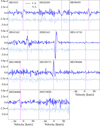 |
Fig. C.1. Least-squares deconvolution profiles for the young, Sun-like stars examined in this work. Each panel corresponds to a different star and contains the Stokes V (solid blue line) and Stokes N (dashed blue line) profiles. The vertical dotted line indicates the radial velocity of the star. We observe that some stars have a clearly detected Zeeman signature (e.g. HD 1835, HD 82443), while others present a flat Stokes V profile (HD 149026, HD 219828), hence they were excluded from tomographic inversion. |
Appendix D: ZDI models of Stokes V profiles
This appendix contains the modelled time series of Stokes V LSD profiles via ZDI. For each star, we show the time series of observed Stokes V profiles, their ZDI models and the rotational cycle computed with Eq. 1. Each profile is shifted vertically for visualisation. In Table D.1, we also include the values of depth, Gaussian width, and Lorentzian width that describe the local Stokes I LSD line profiles. These parameters were optimised via χ2 minimisation between the observed and modelled Stokes I LSD profiles (see Sect. 4).
Optimised Stokes I parameters for ZDI reconstruction.
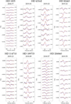 |
Fig. D.1. Stokes V profiles for all stars examined in this work. The cycle number is computed using Eq. 1. For HD 43162 and HD 206860, two columns are shown and correspond to two different epochs. |
All Tables
All Figures
|
Fig. 1. Rotational evolutionary tracks computed by Johnstone et al. (2015a,b) and used in Tu et al. (2015), with our sample stars overplotted. Magenta data points indicate stars with a ZDI map both in the literature and presented in this work, cyan data points indicate stars with a first ZDI reconstruction in this work, and yellow data points indicate stars without a ZDI map. Some of the error bars are smaller than the data point size. The curves represent the 10th (red), 50th (green), and 90th (blue) percentiles of the stellar rotational distribution, of the envelope (solid lines) and core (dotted lines). The small horizontal lines are the observational constraints for the corresponding percentiles. The dashed black line is a time-dependent saturation relation for the stellar dipolar field, the wind mass loss rate and the X-ray luminosity. For more information, see the work of Tu et al. (2015). |
| In the text | |
|
Fig. 2. Joint search of differential rotation and equatorial rotation period for HD 1835, HD 82443, and HD 206860. The panels illustrate the χr2 landscape over a grid of (Prot, eq, dΩ) pairs, with the 1σ and 3σ contours. The best values are obtained by fitting a 2D paraboloid around the minimum, while their error bars are estimated from the projection of the 1σ contour on the respective axis (Press et al. 1992). |
| In the text | |
|
Fig. 3. Reconstructed large-scale magnetic field map of HD 1835, HD 43162, and HD 82443 in flattened polar view. From the left, the radial, azimuthal, and meridional components of the magnetic field vector are illustrated. The radial ticks are located at the rotational phases when the observations were collected (see Eq. (1)), while the concentric circles represent different stellar latitudes: –30 °, +30 °, and +60 ° (dashed lines), as well as the equator (solid line). |
| In the text | |
|
Fig. 4. Reconstructed large-scale magnetic field map of HD 114710, HD 189733, and HD 206860 for the two epochs. The format is the same as Fig. 3. |
| In the text | |
|
Fig. 5. Trends of activity indices and reconstructed magnetic field geometry with age. From the top: logR′HK, average magnetic field strength, poloidal fraction of the total energy, dipolar fraction of the poloidal energy, and axisymmetric fraction of the total energy. Properties measured for the same star but at different epochs are connected by a solid line. Our measurements are represented by ‘X’ and measurements by Folsom et al. (2016, 2018, and references therein) and Bellotti et al. (2025) are indicated with circles. The solar values from the work of Egeland (2017) and Vidotto et al. (2018) are also included. |
| In the text | |
|
Fig. C.1. Least-squares deconvolution profiles for the young, Sun-like stars examined in this work. Each panel corresponds to a different star and contains the Stokes V (solid blue line) and Stokes N (dashed blue line) profiles. The vertical dotted line indicates the radial velocity of the star. We observe that some stars have a clearly detected Zeeman signature (e.g. HD 1835, HD 82443), while others present a flat Stokes V profile (HD 149026, HD 219828), hence they were excluded from tomographic inversion. |
| In the text | |
|
Fig. D.1. Stokes V profiles for all stars examined in this work. The cycle number is computed using Eq. 1. For HD 43162 and HD 206860, two columns are shown and correspond to two different epochs. |
| In the text | |
Current usage metrics show cumulative count of Article Views (full-text article views including HTML views, PDF and ePub downloads, according to the available data) and Abstracts Views on Vision4Press platform.
Data correspond to usage on the plateform after 2015. The current usage metrics is available 48-96 hours after online publication and is updated daily on week days.
Initial download of the metrics may take a while.