| Issue |
A&A
Volume 700, August 2025
|
|
|---|---|---|
| Article Number | A284 | |
| Number of page(s) | 11 | |
| Section | Planets, planetary systems, and small bodies | |
| DOI | https://doi.org/10.1051/0004-6361/202555580 | |
| Published online | 27 August 2025 | |
Insufficient evidence for DMS and DMDS in the atmosphere of K2-18 b
From a joint analysis of JWST NIRISS, NIRSpec, and MIRI observations
Department of Astronomy & Astrophysics, University of Chicago,
Chicago,
IL
60637,
USA
★ Corresponding author: This email address is being protected from spambots. You need JavaScript enabled to view it.
Received:
19
May
2025
Accepted:
3
July
2025
Abstract
Context. Recent JWST observations of the temperate sub-Neptune K2-18 b have been interpreted as suggestive of a liquid water ocean with possible biological activity. Signatures of dimethyl sulfide (DMS) and dimethyl disulfide (DMDS) have been observed in the near-infrared (using the NIRISS and NIRSpec instruments) and mid-infrared (using MIRI). However, the statistical significance of the atmospheric imprints of these potential biomarkers has yet to be quantified from a joint analysis of the entire planet spectrum.
Aims. We aim to test the robustness of the proposed DMS and DMDS detections by simultaneously modeling the NIRISS and NIRSpec observations jointly with the MIRI spectrum for the first time, considering different data reductions and modeling choices.
Methods. We used three well-tested pipelines to re-reduce the JWST observations and two retrieval codes to analyze the resulting transmission spectra as well as previously published data.
Results. The first joint analysis of the panchromatic (0.6–12 µm) spectrum of K2-18 b finds insufficient evidence for the presence of DMS and/or DMDS in the atmosphere of the planet. We find that any marginal preferences are the result of limiting the number of molecules considered in the model and oversensitivity to small changes between data reductions.
Conclusions. Our results confirm that there is no statistical significance for DMS or DMDS in K2-18 b’s atmosphere. While previous works have demonstrated this on MIRI or NIRISS/NIRSpec observations alone, our analysis of the full, panchromatic transmission spectrum does not support claims of potential biomarkers. Using the best-fitting model including DMS and/or DMDS on the published data, we estimate that ∼25 more MIRI transits would be needed for a 3σ rejection of a flat line relative to DMS and/or DMDS features in the planet’s mid-infrared transmission spectrum.
Key words: astrobiology / planets and satellites: atmospheres / planets and satellites: individual: K2-18 b
NHFP Sagan Fellow.
E. Margaret Burbridge postdoctoral fellow.
NSERC postdoctoral fellow.
51 Pegasi b postdoctoral fellow.
These authors have contributed equally to this work.
© The Authors 2025
 Open Access article, published by EDP Sciences, under the terms of the Creative Commons Attribution License (https://creativecommons.org/licenses/by/4.0), which permits unrestricted use, distribution, and reproduction in any medium, provided the original work is properly cited.
This article is published in open access under the Subscribe to Open model. This email address is being protected from spambots. You need JavaScript enabled to view it. to support open access publication.
1 Introduction
The temperate7 sub-Neptune K2-18 b (Montet et al. 2015; Cloutier et al. 2017; Benneke et al. 2017; Sarkis et al. 2018; Cloutier et al. 2019; Radica et al. 2022) continues to be one of the most intensively studied exoplanets in the search for habitable environments beyond the Solar System. Initial Hubble Space Telescope transmission spectroscopy suggested the presence of water vapor in the planet’s atmosphere (Benneke et al. 2019; Tsiaras et al. 2019), though later analyses highlighted degeneracies between H2O and CH4 (Barclay et al. 2021; Blain et al. 2021). With the increased wavelength range of the JWST, Madhusudhan et al. (2023, hereafter M23) reported the detection of CH4 at 5σ and CO2 at 3σ in the H2-rich atmosphere of K2-18 b using data between 0.8 and 5 µm. These findings were interpreted as evidence supporting a hycean scenario – a world covered by a water ocean beneath a thin H2 -rich atmosphere – potentially offering habitable conditions (Piette & Madhusudhan 2020; Madhusudhan et al. 2021).
M23 also reported a low-significance signal from dimethyl sulfide (C2H6S or DMS) – a potential biosignature gas, which has also been found in comets (Hänni et al. 2024) and the interstellar medium (Sanz-Novo et al. 2025) – in their nearinfrared (NIR) spectrum. However, the robustness of these detections, particularly the tentative inference of DMS, is the subject of active scrutiny. A reanalysis of the data presented in M23 by Schmidt et al. (2025, hereafter S25) confirmed CH4 at 4σ, but it found no statistically significant evidence for either CO2 or DMS. Even using the molecular abundances from M23, the hycean interpretation itself has been challenged (Wogan et al. 2024; Shorttle et al. 2024; Huang et al. 2024; Jordan et al. 2025).
More recently, Madhusudhan et al. (2025, hereafter M25) inferred spectral features consistent with DMS and/or dimethyl disulfide (C2H6S2 or DMDS) at 3σ confidence in new midinfrared JWST data from 5 to 12 µm. M25 argued that they represent independent evidence for the presence of sulfurbearing biosignature gases. However, this analysis did not include the existing NIR JWST data, and the statistical robustness of the detection itself was questioned by Taylor (2025) and Welbanks et al. (2025). In this work, we present a reanalysis of the full suite of JWST transmission spectra of K2-18 b to reassess the evidence for DMS and/or DMDS. Advanced data products from this paper can be downloaded from Zenodo.
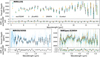 |
Fig. 1 Transmission spectra of K2-18 b from exoTEDRF (blue), JExoRES (black), SPARTA (orange), and Eureka! (green). For NIRISS and NIR-Spec, faded points show higher resolution (R = 100 and 200, respectively) spectra, and solid colors are binned for clarity. Binned points are slightly offset in wavelength for visual clarity. Smaller panels show error-normalized differences relative to exoTEDRF. The JExoRES spectra used a different binning and are interpolated in the difference panels. |
2 Data
The observations of K2-18 b analyzed in this work (and in M23; M25; S25) are part of the JWST GO Program 2722. There are a total of three transit observations: one each with the Near Infrared Imager and Slitless Spectrograph (NIRISS; Doyon et al. 2023) in Single Object Slitless Spectroscopy (SOSS; Albert et al. 2023) mode, the Near Infrared Spectrograph (NIR-Spec; Jakobsen et al. 2022) with the G395H grating, and the Mid-Infrared Instrument (MIRI; Wright et al. 2023) in Low Resolution Spectroscopy (LRS; Bouwman et al. 2023) mode, which yields a continuous 0.6–12 µm spectrum. For more information about the specific observing setups, we invite the reader to consult M23 and M25. In this work, we analyzed the JExoRES pipeline results presented in M23 and M25 and produced independent transmission spectra using exoTEDRF (Radica 2024a) for NIRISS, NIRSpec, and MIRI8; as well as Eureka! (Bell et al. 2022) and SPARTA (Kempton et al. 2023) for NIRSpec and MIRI. Our transmission spectra are shown in Fig. 1. In Appendix A, we summarize relevant choices in each reduction and light-curve modeling from each pipeline.
3 Analysis
We carried out two main modeling analyses. The first is on the JExoRES native-resolution NIRISS and NIRSpec transmission spectra from M23 and the MIRI transmission spectrum from M25. For this, we used PLATON (see Appendix B.1) because it is fast enough to run retrievals at the high spectral resolution required for the pixel-level spectrum. The second is on our independent data reductions with the SCARLET retrieval framework (see Appendix B.2). Clouds (a simple gray deck prescription) and offsets between different JWST detectors are included in all tests. Information on the priors for each retrieval setup is summarized in Table B.1.
We followed Trotta (2008) to assess the statistical significance of our findings using a Bayesian model comparison of log-evidences. Defining ∆ ln Z ≡ ln ZM1 - lnZM0, we used the following thresholds: ∆ lnZ < 1, statistically indistinguishable; ∆ lnZ ∈ [1,2.5), weakly favored; ∆ ln Z ∈ [2.5,5), moderately favored; and ∆ ln Z ≥ 5, strongly favored. We highlight that the direct representation of these values by a sigma value to establish the strength of any detection would be misleading (e.g., Benneke & Seager 2013; Welbanks et al. 2023). A recent article by Kipping & Benneke (2025) summarizes the caveats of converting Bayes factors into frequentist “sigmas” using the table in Benneke & Seager (2013), which is based on earlier papers by Trotta (2008) and ultimately Sellke et al. (2001). Kipping & Benneke (2025) highlights a powerful example in which B = exp(∆ ln Z) = 3 (representing a 3:1 ratio or 25% false-positive rate) yields 2σ using this method, although in frequentist parlance a 2σ significance is associated with a 5% false-positive rate.
PLATON. Starting with a baseline model including CH4, CO2, H2O, NH3, HCN, and CO, we performed five isothermal free retrievals: on the baseline model, one including DMS and DMDS, one with both but excluding MIRI, one without DMS-DMDS but with C2H6 (ethane), and another with all three. The retrieval setup is described in Appendix B.1, while the best-fit models and the abundance posteriors for each molecule are shown in Fig. 2 and Table C.1. While all the PLATON retrievals presented here model the impact of the transit-light-source effect (TLSe; e.g., Rackham et al. 2018) on the spectrum, an identical retrieval was performed without TLSe, which yielded indistinguishable molecular abundance posteriors, in line with the findings of S25.
SCARLET. Given the similarities between the transmission spectra derived in this work (Fig. 1), we only used two combinations for this analysis: one using exoTEDRF for all instruments; and another using exoTEDRF for NIRISS and SPARTA for NIRSpec and MIRI. We performed four isothermal free retrievals on each transmission spectrum using the same baseline model and combinations as before, with and without including MIRI. The retrieval setup is described in Appendix B.2, and the best-fit models and abundance posteriors are shown in Fig. 3 and Table C.1.
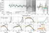 |
Fig. 2 Results from PLATON retrievals performed on transmission spectrum of K2-18 b produced with JExoRES in M23 and M25. Top: transmission spectrum (native-resolution data used in the retrievals in gray; binned data in black for visualization purposes). Best-fit models for the five cases outlined in the text are shown: a baseline model (blue), a model with DMS and DMDS (orange), a model with a common hydrocarbon C2H6 (green), a model with DMS and DMDS but without using the MIRI data (red), and the baseline model with DMS, DMDS, and C2H6 (pink). Models are smoothed to R ∼ 200 for clarity. Bottom: 1D marginalized posterior distributions on molecular species included in each retrieval. Colors reflect the model in the top panel. The black points and vertical dashed lines indicate the abundances reported for each molecule in M23 from just NIRISS and NIRSpec, whereas the gray points in the DMS-DMDS panel indicate the abundances reported in M25 from MIRI data alone. |
4 Results and discussion
Our retrievals of the JExoRES reduction of the 0.8–12 µm transmission spectrum disfavor the presence of DMS and/or DMDS. Including them relatively to a model without those species causes ln Z to decrease by 0.3, indicating no evidence for these species. Data-reduction choices have a moderate impact on the qualitative conclusions. When considering the exoTEDRF and exoTEDRF+SPARTA spectra, the inclusion of DMS and DMDS results in a positive Bayes factor (i.e., ∆ ln Z = 2.1-2.3). Small changes across data reductions at 7 µm (DMS preferred for exoTEDRF+SPARTA) and at 10 µm (DMDS preferred for exoTEDRF-only) are likely responsible for the discrepancy (see top panels in Fig. 3). In no case does the preference for DMS and/or DMDS reach ∆ ln Z > 5, considered standard for any molecule-detection claim. The Bayes factor for each model tested on each transmission-spectrum is shown in Table 1.
The baseline model did not include the many other hydrocarbons expected chemically in the atmosphere of K2-18 b. Thus, our values are likely inflated due to a lack of inclusion of other candidate molecules such as propyne and diethyl sulfide, which have been proposed to explain the MIRI (Welbanks et al. 2025) and NIRISS+NIRSpec (Pica-Ciamarra et al. 2025, hereafter P-C25) spectra, respectively. We considered one additional candidate (ethane) below, as an exhaustive search for all molecules in the full spectrum is beyond the scope of this work.
All reductions (JExoRES, exoTEDRF, exoTEDRF+SPARTA) prefer a high CH4 abundance, but show no evidence of H2 O, NH3, HCN, or CO (Figs. 2 and 3). The SPARTA and JExoRES versions of the spectra yielded bounded posteriors with a slight tail on the CO2 abundance, whereas exoTEDRF yielded much broader CO2 posteriors. The inferred volume-mixing ratios (VMR) in our retrievals on the same data are consistent with those from the “two-offset” case in M23 (CH4 median higher by 1 dex, CO2 by 0.1 dex).
Without DMS and DMDS, we observe a slight posterior peak at high CO abundances in our data reductions, which is still consistent with a non-detection. Since this same peak does not occur in the PLATON retrievals, it may be, instead, an artifact of the model resolution (R = 20 000 was used for SCARLET vs. R = 100 000 for PLATON), as CO is better constrained using the native resolution NIRSpec spectrum (e.g., Esparza-Borges et al. 2023). We highlight that a peak in a posterior does not mean the detection of a chemical absorber (e.g., Welbanks & Madhusudhan 2022).
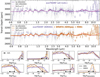 |
Fig. 3 Results from SCARLET retrievals on exoTEDRF and SPARTA where C2H6 is included in the baseline. Top: retrievals performed on exoTEDRF dataset (data in gray, binned in purple). The best-fit model for the retrievals without (with) DMS or DMDS is shown in dark (light) purple, smoothed to R = 200. We show the impact of increasing the C2H6 abundance to 10−2 in the best-fit model from the retrieval without DMS-DMDS as a dashed line. Middle: same, but using SPARTA (orange) for the NIRSpec and MIRI datasets. Bottom: 1D marginalized posterior distributions on the molecular species included in each retrieval. Colors reflect the models at the top. Black error bars and vertical lines (median ±1σ or 2σ upper limits) correspond to the combined POSEIDON results from S25 (which did not include the MIRI data). |
4.1 Uniqueness of DMS and/or DMDS absorption features
Ethane (C2H6) is a common byproduct of methane photolysis by recombining two methyl radicals and the most abundant hydrocarbon predicted by the abiotic photochemistry simulations of K2-18 b in Welbanks et al. (2025). Ethane has a very similar chemical structure to DMS and is ubiquitous in Titan, Jupiter, and Saturn (Nixon et al. 2025). The latter consists of two methyl groups with a sulfur atom in the middle, while the former consists of two directly connected methyl groups. The similarity in molecular structure gives rise to similarities in their absorption cross-sections: the locations of the strongest absorption band in DMS (a C-H stretching mode at 3.4 µm) as well as the second strongest (a H-C-H bending mode at 6.9 µm) are both attributable to the methyl functional group (Table 1.2; Tammer 2004). Therefore, they are present for DMS, DMDS, C2H6 (Fig. 3), and large classes of other organic molecules (Sousa-Silva et al. 2019). In this vein, a recent analysis by Niraula et al. (2025) aptly demonstrates the challenges in detecting hydrocarbons from exoplanet atmospheric retrievals using Titan as an example.
The models with or without ethane are statistically indistinguishable, irrespective of the presence of DMS and/or DMDS (Table 1). Our results support the conclusions in Welbanks et al. (2025) and P-C25 that a wide range of photochemically plausible hydrocarbons could reasonably explain the observations, particularly of the noisy MIRI data.
Summary of model comparison tests using full transmission spectrum (NIRISS+NIRSpec+MIRI).
4.2 Impact of the addition of MIRI/LRS
As shown in Fig. 2, the addition of MIRI data has a negligible impact on the posteriors of all molecules except DMS and DMDS, compared to those from the NIRISS and NIR-Spec data alone. In the JExoRES retrievals, the DMS posterior becomes more sharply peaked around VMR ~10−5 with the addition of MIRI, but it remains an upper limit. For our independent data reductions, the retrievals that do not include MIRI are statistically indistinguishable (∆ ln Z < 1) regardless of the dataset used. The complete results with abundances for NIR-only (NIRISS+NIRSpec) tests are shown in Table C.2.
Furthermore, we retrieved photospheric temperatures much lower than the  K at 1 mbar inferred by M25 from the MIRI data alone – which is inconsistent with the predicted zero-albedo, no-atmosphere substellar temperature of
  K. This conclusion is supported regardless of the adopted photosphere temperature prior adopted9 and across PLATON and SCARLET retrievals. This discrepancy is driven by the fact that the apparent “features” in the MIRI spectrum are much larger than the spectral features at bluer wavelengths. If they were indeed from the planet, the atmosphere would need to be relatively hot to have a sufficiently large scale height. However, this is inconsistent with both energy balance and the more precise NIRISS and NIRSpec observations. Therefore, while the MIRI features are suggestive of DMS, DMDS, or other hydrocarbons, and thus increase the evidence for these species in the retrievals, the features are implausibly large.
We performed a suite of simulations to determine how many MIRI transits would be needed to robustly detect spectral features, assuming the best-fitting model from the PLATON DMS-DMDS retrieval on the JExoRES spectrum represents the underlying atmosphere. We find that an average of 26 transits have to be stacked to obtain a 3σ rejection of a flat line when scaling the JExoRES errors. However, this result is highly sensitive to the noise realization, and the standard deviation of the number of transits needed in 1000 simulations is 13. We note that due to the star’s position in the sky and the long orbital period of the planet, there are typically only three transit opportunities observable with the JWST each year.
5 Conclusions
K2-18 b is undoubtedly one of the most promising planets for interior, atmosphere, and habitability studies of a sub-Neptune in the JWST era. Transmission spectroscopy robustly finds CH4 in its hydrogen-rich atmosphere, but the presence of other species is still under debate. In this letter, we provide an independent analysis at both the data reduction and atmospheric modeling levels, leveraging the full wavelength coverage (0.6–12 µm) publicly available for this planet for the first time. We can reproduce the abundances reported by M23 for CH4 and CO2 using either the previous spectrum or our independent reductions, although the exact abundance of CO2 is influenced by the specific pipeline used. DMS and/or DMDS are not detected robustly across different data reductions or molecules included in the baseline model, consistent with the results from P-C25 for NIRISS/NIRSpec when adding instrumental offsets and Welbanks et al. (2025) for MIRI.
Regarding DMS and/or DMDS, we note that there are no cross-sections yet available for pressures lower than 1 bar, which would be more representative of the upper atmosphere probed in transmission, and this leads to overestimated absorption features. Conversely, the line lists for most organic molecules and hydrocarbons, including ethane, are extremely incomplete to date, which can lead to an underestimation of their absorption signal. The clear deficiencies in the current line lists highlight the need for further experimental and theoretical studies to address them, particularly as next-generation facilities including HWO and the ELTs aim to supercharge the search for habitable conditions on other planets.
Data availability
Advanced data products from this paper can be downloaded from Zenodo.
Acknowledgements
The authors would like to thank Guangwei Fu, Matt Nixon, Brandon Park Coy, Vivien Parmentier, and Luis Welbanks for helpful discussions. This work is based on observations made with the NASA/ESA/CSA James Webb Space Telescope. The data were obtained from the Mikulski Archive for Space Telescopes at the Space Telescope Science Institute, which is operated by the Association of Universities for Research in Astronomy, Inc., under NASA contract NAS 5-03127 for JWST. R.L. is supported by NASA through the NASA Hubble Fellowship grant HST-HF2-51559.001-A awarded by the Space Telescope Science Institute, which is operated by the Association of Universities for Research in Astronomy, Inc., for NASA, under contract NAS5-26555. M.Z. and M.E.S. thank the Heising-Simons Foundation for support through the 51 Pegasi b fellowship. C.P.-G. is supported by the E. Margaret Burbidge Prize Postdoctoral Fellowship from the Brinson Foundation. D.S. acknowledges funding as part of JWST GO program 3969 (PIs: Espinoza, Powell). M.R. acknowledges financial support from the Natural Sciences and Engineering Research Council of Canada through a Postdoctoral Fellowship. He would also like to thank Hannah Wakeford and David Grant for useful conversations about MIRI systematics.
Appendix A Reduction details
A.1 JExoRES
We use the NIRISS/SOSS and NIRSpec/G395H spectra presented in M23 using JExoRES (Holmberg & Madhusudhan 2023) that can be downloaded here. For the MIRI/LRS spectra, we use the JExoRES version presented in M25 that can be downloaded here. The JexoPipe pipeline (Sarkar et al. 2024) was also used in M25, but these results are not public.
A.2 exoTEDRF
As of release 2.3.0, exoTEDRF (Radica 2024a; Radica et al. 2023; Feinstein et al. 2023) is now the first publicly available pipeline for exoplanet time series observations with full support for NIRISS, NIRSpec, and MIRI. We thus make use of exoTEDRF to produce a 0.6 – 12 µm spectrum with a single data analysis framework.
A.2.1 NIRISS/SOSS & NIRSpec/G395H
We use the NIRISS/SOSS and NIRSpec/G395H exoTEDRF spectra from S25. For details on the data reduction and light curve analysis, we point the reader to Sections 2.2, 3.2, and Table 1 of that work. Here, we use the transmission spectrum computed at a resolution of R = 100 for NIRISS and R = 200 for NIRSpec. This choice is motivated by the analysis in S25 (their Fig. 5) showing that this is the configuration that results in the highest detection significances of CH4, CO2, and DMS.
A.2.2 MIRI/LRS
As this is the first use of exoTEDRF for MIRI observations, we briefly describe the methodology below, and refer the reader to Radica et al. (in prep.) for more details.
In Stage 1, we perform data quality and saturation flagging, EMI correction, linearity correction, dark current subtraction, cosmic ray flagging, and ramp fitting. During linearity correction, we flag the first five and last groups up-the-ramp as DO_NOT_USE before proceeding with the linearity correction using the default STScI polynomials. As in M25, we find that applying a linearity self-calibration results in a consistent spectrum, as does varying the number of groups clipped at the start of the ramp. Cosmic ray identification is performed using a timedomain rejection algorithm, and a 7σ threshold (Radica et al. 2024). All other steps are the exoTEDRF defaults. We skip the gain scale correction since absolute flux values are not necessary for this work.
In Stage 2, we assign the WCS and source type, correct flat fielding effects, and interpolate bad pixels. We subtract the background using a row-wise median, calculated from two 14-pixel-wide regions on either side of the trace (columns 12–26 and 46–60). Finally, we perform a PCA reconstruction on the combined TSO data cube. This is similar to analyses performed by Coulombe et al. (2023) and Radica et al. (2024), except instead of using the PCA eigenvalue timeseries as vectors against which to detrend during light curve fitting, we reconstruct the 3D time series (i.e., integration number, X-pixel, Y-pixel), removing components which are correlated with detector trends. For this particular timeseries, we remove the second component, which is correlated with a sub-pixel drift along the detector X (i.e., spatial) axis. Finally, we trace the spectrum on the detector using the edgetrigger algorithm (Radica et al. 2022), and perform a box aperture extraction with a width of six pixels, clipping 4σ outliers from the resulting light curves.
We fit the light curves using the exoUPRF library (Radica 2024b; Radica et al. 2025). The white light curve is constructed using wavelengths 5–12 µm. For the astrophysical transit model, we use a standard batman model (Kreidberg 2015). We fix the period to 32.940045 d (Benneke et al. 2019), and put Gaussian priors on the orbital parameters based on the best fitting values in M23. The limb darkening is freely fit in the range u1, u2 ∈ [−1,1] using the quadratic law. We include a systematics model consisting of an exponential ramp and linear slope, as well as an error inflation term added in quadrature to the extracted flux errors.
For the spectroscopic fits, we bin the light curves in increments of 0.25 µm (R ∼ 100), yielding 28 bins across the 5– 12 µm range. We fix the orbital parameters to the best-fitting values from the white light fits, and allow the scaled planet radius, transit zero point, error inflation, and two of the three parameters of the systematics model (linear slope and amplitude of exponential ramp) to vary freely. We, however, fix the exponential ramp timescale to the best-fitting values from the white light fit, as it remains unconstrained otherwise. We fix the two parameters of the quadratic limb darkening law to predictions from ExoTiC-LD (Grant & Wakeford 2022) using MPS-ATLAS2 stellar models (Kostogryz et al. 2022). We also cut the first 250 integrations from each spectroscopic light curve as in M25.
A.3 Eureka!
A.3.1 NIRSpec/G395H
We reduce the observations and fit the spectroscopic light curves using an identical setup as the “Eureka! B” analysis in S25. For this work, we compute a set of spectroscopic light curves at R = 200 (not made publicly available) for direct comparison with the other reductions. The control and parameter files for Stages 4–6 are available for download from Zenodo.
A.3.2 MIRI/LRS
We start with the uncalibrated files and run Stages 1–2, which are wrappers of the STScI jwst pipeline. We use default steps (data quality initialization, electromagnetic interference correction, saturation flagging, discard first and last frames, linearity correction, reset switch charge decay correction, dark current subtraction, and ramp fitting) and a 15σ threshold in the jump step. We do not perform group-level background subtraction. We skip the flat-field correction in Stage 2. We then extract the stellar time-series spectra in Stage 3. We perform a mean column-by-column background subtraction, excluding the area within 10 pixels of the center of the trace. We use an aperture of 9 pixels, corresponding to a 4-pixel half width, to optimally extract (Horne 1986) the time-series spectra. In Stage 4, we generate broadband (white light, covering 5.24–12.02 µm) and spectroscopic light curves using a bin width of 0.25 µm (between 5–12 µm, equaling 28 spectroscopic bins).
In Stage 5, we fit the white light curve using an exponential ramp and a linear trend as the systematics model. We mask the first 250 integrations to remove the strongest effect of the detector settling, assume a circular orbit, fix the period to 32.940043 d (Benneke et al. 2019), and give uninformative priors to the rest of the parameters (t0, a/R⋆, i, Rp/R⋆, q1, and q2). We use a quadratic limb darkening law parameterized as in Kipping (2013). We add in quadrature an error inflation term to the extracted flux errors. Our choices mimic those of the final JExoRES reduction of M25. Our best-fit parameters are consistent within 1σ with those of that work, except for a/R⋆ where we find 78.8 ± 1.1 as opposed to 80.3 ± 0.5 in M25. To obtain the transmission spectrum, we fix all orbital parameters (except Rp/R⋆ and the parameters associated with the systematics model) to the values from our white light curve analysis. We include the control and parameter files for Stages 1–6, as well as the white light curve and best-fit parameters of their model, in Zenodo to verify all our choices and reproduce these results.
A.4 SPARTA
SPARTA is an end-to-end data reduction and analysis pipeline for JWST. Starting from the _uncal.fits files, SPARTA operates completely independently of the official JWST pipeline (Bushouse et al. 2023) and is 27 times faster than the calwebb_detector1 (JWST Stage 1) code. In this paper, we re-analyze both the NIRSpec and MIRI/LRS data using SPARTA.
A.4.1 NIRSpec/G395H
We generate the _rateints.fits files following the same procedure described in Kempton et al. (2023), which includes applying the superbias (reference file version of 0479 for NRS1, 0474 for NRS2), correcting with the reference pixels, applying the non-linearity correction (0024), subtracting the dark current (0457/0470), masking bad pixels (0082/0080), multiplying by the gain (0025/0027), fitting the slope, subtracting the residuals, and re-fitting the slope. The only deviation from Kempton et al. (2023) is the addition of a group-level background subtraction step before slope fitting. To perform this, we first identified the Gaussian center of the 2D spectra via least-squares fitting. We then masked a region within seven pixels of the center and subtracted the median of the remaining background region from the entire image.
After generating the _rateints.fits files, we applied a second background subtraction using the same group-level strategy and measured the x- and y-positions of the spectral trace from the cleaned median frame. We then performed optimal extraction over columns 610–2044 of NRS1 and columns 4– 2044 of NRS2, covering wavelength ranges of 2.749–3.717 µm and 3.823–5.100 µm, respectively. Following extraction, we interpolated over bad rows and removed bad rows and columns. As a final step in the reduction, we computed a detrended light curve by subtracting a median-filtered light curve (kernel size 50). Integrations deviating by more than 3σ from zero in the detrended light curve were flagged as bad.
For light curve fitting, we fixed t0, P, a/R⋆, and i to the values listed in Table 1 of M23. We binned the light curves to a resolving power of R ∼ 200, resulting in 123 spectroscopic channels. The first 30 integrations were discarded. We modeled systematics using Fsys = F⋆(1 + m(t - t̄) + cyy + cxx), where we account for a linear trend with time and detector positional systematics. We treated the limb darkening coefficients as free parameters and fitted them using the formalism of Kipping (2013).
A.4.2 MIRI/LRS
We reduced the MIRI/LRS data following the same procedure described in the NIRSpec section, with two exceptions: MIRI does not require a superbias correction, and we did not apply group-level background subtraction. For a more detailed description of the SPARTA MIRI/LRS reduction, we refer readers to Kempton et al. (2023), Zhang et al. (2024), and Xue et al. (2024). The calibration reference files used were: non-linearity (version 0032), dark current (0102), mask (0036), and gain (0042). For integration-level background subtraction, we computed the median value of rows [10, 21] and [−21, −10], and subtracted this value from each integration.
Optimal extraction was performed within five pixels of the trace, from column 20 to 275. We applied the same spectral binning as in the exoTEDRF and Eureka! reductions. For the spectroscopic light curve fitting, we fixed t0, a/R⋆, i, u1, and u2 to the best-fit values derived from the wavelength-integrated white light curve: 60426.12880 d (BJD - 2400000.5), 78.87, 89.53 deg, 0.0352, and 0.1083, respectively. The first 250 integrations were excluded from the fitting. We adopted  as the systematics model where we account for ramp-like behavior and detector positional variation, as it yielded the lowest RMS residuals among the various models we tested.
Appendix B Retrieval setup
Fixed and free parameters in the PLATON and SCARLET retrievals.
B.1 PLATON
PLATON is a GPU-accelerated atmospheric retrieval code (Zhang et al. 2019, 2020, 2025) that has been used in numerous works, including for JWST transmission spectra of miniNeptunes (e.g., Davenport et al. 2025). We use the latest version of the code (6.3.1), except that we significantly speed up the method that bins the model transit spectrum to the observed wavelength bins.
The default PLATON opacities are at a spectral resolution of 20,000, which is too low to retrieve on the native-resolution NIRISS and NIRSpec spectra. They have a temperature spacing of 100 K, uncomfortably coarse for a planet as cold as K2-18b. We replace them with R = 100,000 opacities generated from the DACE opacity database4, and halve the temperature spacing to 50 K. For CH4, we use the HITEMP 2020 line list (Hargreaves et al. 2020), which (unlike the ExoMol line lists) covers the entire wavelength range spanned by the NIRISS data. C2H6 is not in the DACE database, so we compute absorption cross sections with ExoCross from the HITRAN 2020 line list (Gordon et al. 2022a). DMS and DMDS have no published line lists, so we assume the absorption cross sections measured at 278 K in a 1 bar nitrogen atmosphere by Sharpe et al. (2004) are valid at all temperatures and pressures. Because these cross sections are far more pressure broadened at 1 bar than at K2-18 b’s photospheric pressure of ∼1 mbar, we expect the retrieval to overestimate absorption and thus underestimate the DMS/DMDS abundance. On the other hand, the C2H6 line list is highly incomplete, likely leading to underestimation of absorption and overestimation of its abundance.
We perform a free retrieval via nested sampling with an isothermal atmosphere, an opaque cloud deck, transit light source effect (TLSe) from starspots, and three instrumental offsets relative to NRS2 (NIRISS, NRS1, MIRI). The TLSe is parameterized with a starspot temperature and a starspot covering fraction, with the non-spotted surface fixed at the Teff of 3457 K (Cloutier et al. 2017). Both the starspot spectrum and the non-starspot spectrum are obtained from the BT-Settl (AGSS2009) spectral grid that is included in PLATON. Our formalism could allow for Tspot to go above Teff and account for faculae contamination. However, S25 explored models with both 1- and 2-component heterogeneities and found that a very small fraction of the posterior samples (< 1%) on the starspot temperature were hotter than the stellar photosphere temperature (their Fig. 7). The Tspot posterior samples from our analyses are also strongly peaked toward low temperatures, in line with S25. All fixed and free parameters, together with the priors assumed for the free parameters, are listed in Table B.1. The nested sampling was performed by pymultinest with 1000 live points (Buchner et al. 2014). We used the Bayesian evidence reported by Importance Nested Sampling, which can calculate the evidence with up to an order of magnitude higher accuracy (Feroz et al. 2019).
In our analyses, we found that when temperatures down to 100 K are allowed, the retrievals obtain a surprisingly low photosphere temperature, with medians and error bars within 5 K of 175-40 K. However, the posteriors are sufficiently broad that the temperature is 2σ consistent with the equilibrium temperature of ∼250 K. To explore the effect of forcing higher temperatures, we perform a retrieval with DMS/DMDS where we impose a minimum temperature of 100 K instead of 200 K. This slightly lowers the upper limits on DMS and DMDS, by 0.35 and 0.57 dex, respectively. It also decreases the median CH4 abundance by 0.23 dex, making it more similar to the SCARLET results.
B.2 SCARLET
We analyze our independently derived transmission spectra with the SCARLET atmospheric retrieval framework (Benneke & Seager 2012, 2013; Benneke 2015; Benneke et al. 2019; Roy et al. 2023) including modifications for more flexible modeling of sub-Neptune atmospheres (Piaulet et al. 2023; Piaulet-Ghorayeb et al. 2024). We elect to perform free retrievals, where we fit for well-mixed abundances of the gaseous species making up the atmosphere. This approach does not require that the relative abundances match chemical equilibrium, which might not be a valid assumption in the upper atmospheres of colder sub-Neptunes (Wogan et al. 2024; Benneke et al. 2024).
Our forward model iterates over the radiative transfer and hydrostatic equilibrium calculation to determine the altitudepressure mapping consistent with the temperature structure and composition prescribed by the fitted parameters. We include H2, He, HCN, H2O, CO, CO2, CH4, NH3, and C2H6 in our nominal set of molecules. We perform additional tests that include DMS and DMDS. For absorbing species, we use the cross sections from HELIOS-K for H2O (Polyansky et al. 2018), CO (Hargreaves et al. 2019), CO2 (Yurchenko et al. 2020), CH4 (Hargreaves et al. 2020), HCN (Harris et al. 2006), NH3 (Coles et al. 2019). The C2H6 cross-sections are computed from the HITRAN line lists (Gordon et al. 2022b). For DMS and DMDS, where no line lists are available, we use the 278.15 K crosssections from the HITRAN database (Sharpe et al. 2004). The abundances of absorbing species are fitted as parameters, while H2/He is treated as a filler gas making up the remainder for an atmosphere (with a Jupiter-like ratio He/H2 = 0.157).
Contrary to emission spectra, transmission spectra struggle to constrain gradients in the vertical temperature structure of sub-Neptunes. This motivates us to adopt the standard prescription of instead fitting only one temperature Tp (the scale height temperature) to be near-constant over the limited pressure range probed in transmission. To account for aerosol obfuscation, we use a gray cloud deck (fitting the pressure below which the atmosphere becomes opaque) and hazes following Lecavelier Des Etangs et al. (2008). We do not include stellar contamination in our model, since the deeper analysis from S25 found that its inclusion does not impact the inferred properties from the NIRISS+NIRSpec data. The longer wavelengths probed by MIRI are not sensitive to stellar contamination. We allow for three offsets between instruments/detectors relative to NIRISS/SOSS: one for the NRS1 detector of NIRSpec/G395H, one for the NRS2 detector of NIRSpec/G395H, and another for MIRI/LRS. We also fit the planet mass with a Gaussian prior on the value reported by Benneke et al. (2019).
For each combination of model parameters, we optimize the value of the 10 mbar radius until the best data-model match is achieved, iterating over both the hydrostatic equilibrium and radiative transfer steps. The parameter space is sampled using multi-ellipsoid nested sampling as implemented in the nestle module (Skilling 2004, 2006). We compute models at a resolving power of 20,000, appropriate for the 100–200 resolving power of the data at hand. Each model is then convolved to the resolution of the observed spectrum for the likelihood evaluation.
Appendix C Molecular abundances
Retrieved molecular abundances of prominent molecules in the atmosphere of K2-18 b.
References
- Albert, L., Lafrenière, D., Doyon, R., et al. 2023, PASP, 135, 075001 [Google Scholar]
- Barclay, T., Kostov, V. B., Colón, K. D., et al. 2021, AJ, 162, 300 [NASA ADS] [CrossRef] [Google Scholar]
- Bell, T., Ahrer, E.-M., Brande, J., et al. 2022, J. Open Source Softw., 7, 4503 [NASA ADS] [CrossRef] [Google Scholar]
- Benneke, B. 2015, arXiv e-prints [arXiv:1504.07655] [Google Scholar]
- Benneke, B., & Seager, S. 2012, ApJ, 753, 100 [NASA ADS] [CrossRef] [Google Scholar]
- Benneke, B., & Seager, S. 2013, ApJ, 778, 153 [Google Scholar]
- Benneke, B., Werner, M., Petigura, E., et al. 2017, ApJ, 834, 187 [Google Scholar]
- Benneke, B., Wong, I., Piaulet, C., et al. 2019, ApJ, 887, L14 [Google Scholar]
- Benneke, B., Roy, P.-A., Coulombe, L.-P., et al. 2024, arXiv e-prints [arXiv:2403.03325] [Google Scholar]
- Blain, D., Charnay, B., & Bézard, B. 2021, A&A, 646, A15 [EDP Sciences] [Google Scholar]
- Bouwman, J., Kendrew, S., Greene, T. P., et al. 2023, PASP, 135, 038002 [NASA ADS] [CrossRef] [Google Scholar]
- Buchner, J., Georgakakis, A., Nandra, K., et al. 2014, A&A, 564, A125 [NASA ADS] [CrossRef] [EDP Sciences] [Google Scholar]
- Bushouse, H., Eisenhamer, J., Dencheva, N., et al. 2023, https://doi.org/10.5281/zenodo.8404029 [Google Scholar]
- Cloutier, R., Astudillo-Defru, N., Doyon, R., et al. 2017, A&A, 608, A35 [NASA ADS] [CrossRef] [EDP Sciences] [Google Scholar]
- Cloutier, R., Astudillo-Defru, N., Doyon, R., et al. 2019, A&A, 621, A49 [NASA ADS] [CrossRef] [EDP Sciences] [Google Scholar]
- Coles, P. A., Yurchenko, S. N., & Tennyson, J. 2019, MNRAS, 490, 4638 [CrossRef] [Google Scholar]
- Coulombe, L.-P., Benneke, B., Challener, R., et al. 2023, Nature, 620, 292 [NASA ADS] [CrossRef] [Google Scholar]
- Davenport, B., Kempton, E. M. R., Nixon, M. C., et al. 2025, ApJ, 984, L44 [Google Scholar]
- Doyon, R., Willott, C. J., Hutchings, J. B., et al. 2023, PASP, 135, 098001 [NASA ADS] [CrossRef] [Google Scholar]
- Esparza-Borges, E., López-Morales, M., Adams Redai, J. I., et al. 2023, ApJ, 955, L19 [NASA ADS] [CrossRef] [Google Scholar]
- Feinstein, A. D., Radica, M., Welbanks, L., et al. 2023, Nature, 614, 670 [NASA ADS] [CrossRef] [Google Scholar]
- Feroz, F., Hobson, M. P., Cameron, E., & Pettitt, A. N. 2019, Open J. Astrophys., 2, 10 [Google Scholar]
- Gordon, I. E., Rothman, L. S., Hargreaves, R. J., et al. 2022a, J. Quant. Spectrosc. Radiat. Transf., 277, 107949 [NASA ADS] [CrossRef] [Google Scholar]
- Gordon, I. E., Rothman, L. S., Hargreaves, R. J., et al. 2022b, J. Quant. Spec. Radiat. Transf., 277, 107949 [NASA ADS] [CrossRef] [Google Scholar]
- Grant, D., & Wakeford, H. R. 2022, https://doi.org/10.5281/zenodo.7437681 [Google Scholar]
- Hänni, N., Altwegg, K., Combi, M., et al. 2024, ApJ, 976, 74 [Google Scholar]
- Hargreaves, R. J., Gordon, I. E., Rothman, L. S., et al. 2019, J. Quant. Spec. Radiat. Transf., 232, 35 [NASA ADS] [CrossRef] [Google Scholar]
- Hargreaves, R. J., Gordon, I. E., Rey, M., et al. 2020, ApJS, 247, 55 [NASA ADS] [CrossRef] [Google Scholar]
- Harris, G. J., Tennyson, J., Kaminsky, B. M., Pavlenko, Y. V., & Jones, H. R. A. 2006, MNRAS, 367, 400 [Google Scholar]
- Holmberg, M., & Madhusudhan, N. 2023, MNRAS, 524, 377 [NASA ADS] [CrossRef] [Google Scholar]
- Horne, K. 1986, PASP, 98, 609 [Google Scholar]
- Huang, Z., Yu, X., Tsai, S.-M., et al. 2024, ApJ, 975, 146 [Google Scholar]
- Jakobsen, P., Ferruit, P., Alves de Oliveira, C., et al. 2022, A&A, 661, A80 [NASA ADS] [CrossRef] [EDP Sciences] [Google Scholar]
- Jordan, S., Shorttle, O., & Quanz, S. P. 2025, arXiv e-prints [arXiv:2504.12030] [Google Scholar]
- Kempton, E. M. R., Zhang, M., Bean, J. L., et al. 2023, Nature, 620, 67 [NASA ADS] [CrossRef] [Google Scholar]
- Kipping, D. M. 2013, MNRAS, 435, 2152 [Google Scholar]
- Kipping, D., & Benneke, B. 2025, arXiv e-prints [arXiv:2506.05392] [Google Scholar]
- Kostogryz, N. M., Witzke, V., Shapiro, A. I., et al. 2022, A&A, 666, A60 [NASA ADS] [CrossRef] [EDP Sciences] [Google Scholar]
- Kreidberg, L. 2015, PASP, 127, 1161 [Google Scholar]
- Lecavelier Des Etangs, A., Pont, F., Vidal-Madjar, A., & Sing, D. 2008, A&A, 481, L83 [NASA ADS] [CrossRef] [Google Scholar]
- Madhusudhan, N., Piette, A. A. A., & Constantinou, S. 2021, ApJ, 918, 1 [NASA ADS] [CrossRef] [Google Scholar]
- Madhusudhan, N., Sarkar, S., Constantinou, S., et al. 2023, ApJ, 956, L13 [NASA ADS] [CrossRef] [Google Scholar]
- Madhusudhan, N., Constantinou, S., Holmberg, M., et al. 2025, ApJ, 983, L40 [Google Scholar]
- Montet, B. T., Morton, T. D., Foreman-Mackey, D., et al. 2015, ApJ, 809, 25 [Google Scholar]
- Niraula, P., de Wit, J., Hargreaves, R., Gordon, I. E., & Sousa-Silva, C. 2025, arXiv e-prints [arXiv:2506.12144] [Google Scholar]
- Nixon, C. A., Bézard, B., Cornet, T., et al. 2025, Nat. Astron., 9, 969 [Google Scholar]
- Piaulet, C., Benneke, B., Almenara, J. M., et al. 2023, Nat. Astron., 7, 206 [Google Scholar]
- Piaulet-Ghorayeb, C., Benneke, B., Radica, M., et al. 2024, ApJ, 974, L10 [NASA ADS] [CrossRef] [Google Scholar]
- Pica-Ciamarra, L., Madhusudhan, N., Cooke, G. J., Constantinou, S., & Binet, M. 2025, arXiv e-prints [arXiv:2505.10539] [Google Scholar]
- Piette, A. A. A., & Madhusudhan, N. 2020, MNRAS, 497, 5136 [Google Scholar]
- Polyansky, O. L., Kyuberis, A. A., Zobov, N. F., et al. 2018, MNRAS, 480, 2597 [NASA ADS] [CrossRef] [Google Scholar]
- Rackham, B. V., Apai, D., & Giampapa, M. S. 2018, ApJ, 853, 122 [Google Scholar]
- Radica, M. 2024a, J. Open Source Softw., 9, 6898 [Google Scholar]
- Radica, M. 2024b, https://doi.org/10.5281/zenodo.12628066 [Google Scholar]
- Radica, M., Albert, L., Taylor, J., et al. 2022, PASP, 134, 104502 [Google Scholar]
- Radica, M., Artigau, É., Lafreniére, D., et al. 2022, MNRAS, 517, 5050 [NASA ADS] [CrossRef] [Google Scholar]
- Radica, M., Welbanks, L., Espinoza, N., et al. 2023, MNRAS, 524, 835 [NASA ADS] [CrossRef] [Google Scholar]
- Radica, M., Coulombe, L.-P., Taylor, J., et al. 2024, ApJ, 962, L20 [NASA ADS] [CrossRef] [Google Scholar]
- Radica, M., Piaulet-Ghorayeb, C., Taylor, J., et al. 2025, ApJ, 979, L5 [NASA ADS] [CrossRef] [Google Scholar]
- Roy, P.-A., Benneke, B., Piaulet, C., et al. 2023, ApJ, 954, L52 [NASA ADS] [CrossRef] [Google Scholar]
- Sanz-Novo, M., Rivilla, V. M., Endres, C. P., et al. 2025, ApJ, 980, L37 [Google Scholar]
- Sarkar, S., Madhusudhan, N., Constantinou, S., & Holmberg, M. 2024, MNRAS, 531, 2731 [Google Scholar]
- Sarkis, P., Henning, T., Kürster, M., et al. 2018, AJ, 155, 257 [NASA ADS] [CrossRef] [Google Scholar]
- Schmidt, S. P., MacDonald, R. J., Tsai, S.-M., et al. 2025, arXiv e-prints [arXiv:2501.18477] [Google Scholar]
- Sellke, T., Bayarri, M. J., & Berger, J. O. 2001, Am. Statist., 55, 62 [Google Scholar]
- Sharpe, S. W., Johnson, T. J., Sams, R. L., et al. 2004, Appl. Spectrosc., 58, 1452 [NASA ADS] [CrossRef] [Google Scholar]
- Shorttle, O., Jordan, S., Nicholls, H., Lichtenberg, T., & Bower, D. J. 2024, ApJ, 962, L8 [NASA ADS] [CrossRef] [Google Scholar]
- Skilling, J. 2004, in AIP Con. Proc., 735, Entropy Methods in Science and Engineering, eds. R. Fischer, R. Preuss, & U. V. Toussaint (AIP), 395 [Google Scholar]
- Skilling, J. 2006, Bayesian Anal., 1, 833 [Google Scholar]
- Sousa-Silva, C., Petkowski, J. J., & Seager, S. 2019, Phys. Chem. Chem. Phys., 21, 18970 [Google Scholar]
- Tammer, M. 2004, Colloid Polym. Sci., 283, 235 [Google Scholar]
- Taylor, J. 2025, RNAAS, 9, 118 [Google Scholar]
- Trotta, R. 2008, Contemp. Phys., 49, 71 [Google Scholar]
- Tsiaras, A., Waldmann, I. P., Tinetti, G., Tennyson, J., & Yurchenko, S. N. 2019, Nat. Astron., 3, 1086 [Google Scholar]
- Welbanks, L., & Madhusudhan, N. 2022, ApJ, 933, 79 [NASA ADS] [CrossRef] [Google Scholar]
- Welbanks, L., McGill, P., Line, M., & Madhusudhan, N. 2023, AJ, 165, 112 [NASA ADS] [CrossRef] [Google Scholar]
- Welbanks, L., Nixon, M. C., McGill, P., et al. 2025, arXiv e-prints [arXiv:2504.21788] [Google Scholar]
- Wogan, N. F., Batalha, N. E., Zahnle, K. J., et al. 2024, ApJ, 963, L7 [NASA ADS] [CrossRef] [Google Scholar]
- Wright, G. S., Rieke, G. H., Glasse, A., et al. 2023, PASP, 135, 048003 [NASA ADS] [CrossRef] [Google Scholar]
- Xue, Q., Bean, J. L., Zhang, M., et al. 2024, ApJ, 963, L5 [NASA ADS] [CrossRef] [Google Scholar]
- Yurchenko, S. N., Mellor, T. M., Freedman, R. S., & Tennyson, J. 2020, MNRAS, 496, 5282 [NASA ADS] [CrossRef] [Google Scholar]
- Zhang, M., Chachan, Y., Kempton, E. M. R., & Knutson, H. A. 2019, PASP, 131, 034501 [Google Scholar]
- Zhang, M., Chachan, Y., Kempton, E. M. R., Knutson, H. A., & Chang, W. H. 2020, ApJ, 899, 27 [CrossRef] [Google Scholar]
- Zhang, M., Hu, R., Inglis, J., et al. 2024, ApJ, 961, L44 [NASA ADS] [CrossRef] [Google Scholar]
- Zhang, M., Paragas, K., Bean, J. L., et al. 2025, AJ, 169, 38 [Google Scholar]
Teq = 255 ± 4 K assuming 0.3 Bond albedo (Benneke et al. 2019).
exoTEDRF v2.3.0 adds support for MIRI, making it (at the time of writing) the only publicly available pipeline to fully support NIRISS, NIRSpec, and MIRI.
See Appendix B.1 for a discussion on the temperature priors and posterior constraints.
All Tables
Summary of model comparison tests using full transmission spectrum (NIRISS+NIRSpec+MIRI).
Retrieved molecular abundances of prominent molecules in the atmosphere of K2-18 b.
All Figures
|
Fig. 1 Transmission spectra of K2-18 b from exoTEDRF (blue), JExoRES (black), SPARTA (orange), and Eureka! (green). For NIRISS and NIR-Spec, faded points show higher resolution (R = 100 and 200, respectively) spectra, and solid colors are binned for clarity. Binned points are slightly offset in wavelength for visual clarity. Smaller panels show error-normalized differences relative to exoTEDRF. The JExoRES spectra used a different binning and are interpolated in the difference panels. |
| In the text | |
|
Fig. 2 Results from PLATON retrievals performed on transmission spectrum of K2-18 b produced with JExoRES in M23 and M25. Top: transmission spectrum (native-resolution data used in the retrievals in gray; binned data in black for visualization purposes). Best-fit models for the five cases outlined in the text are shown: a baseline model (blue), a model with DMS and DMDS (orange), a model with a common hydrocarbon C2H6 (green), a model with DMS and DMDS but without using the MIRI data (red), and the baseline model with DMS, DMDS, and C2H6 (pink). Models are smoothed to R ∼ 200 for clarity. Bottom: 1D marginalized posterior distributions on molecular species included in each retrieval. Colors reflect the model in the top panel. The black points and vertical dashed lines indicate the abundances reported for each molecule in M23 from just NIRISS and NIRSpec, whereas the gray points in the DMS-DMDS panel indicate the abundances reported in M25 from MIRI data alone. |
| In the text | |
|
Fig. 3 Results from SCARLET retrievals on exoTEDRF and SPARTA where C2H6 is included in the baseline. Top: retrievals performed on exoTEDRF dataset (data in gray, binned in purple). The best-fit model for the retrievals without (with) DMS or DMDS is shown in dark (light) purple, smoothed to R = 200. We show the impact of increasing the C2H6 abundance to 10−2 in the best-fit model from the retrieval without DMS-DMDS as a dashed line. Middle: same, but using SPARTA (orange) for the NIRSpec and MIRI datasets. Bottom: 1D marginalized posterior distributions on the molecular species included in each retrieval. Colors reflect the models at the top. Black error bars and vertical lines (median ±1σ or 2σ upper limits) correspond to the combined POSEIDON results from S25 (which did not include the MIRI data). |
| In the text | |
Current usage metrics show cumulative count of Article Views (full-text article views including HTML views, PDF and ePub downloads, according to the available data) and Abstracts Views on Vision4Press platform.
Data correspond to usage on the plateform after 2015. The current usage metrics is available 48-96 hours after online publication and is updated daily on week days.
Initial download of the metrics may take a while.