| Issue |
A&A
Volume 701, September 2025
|
|
|---|---|---|
| Article Number | A185 | |
| Number of page(s) | 9 | |
| Section | The Sun and the Heliosphere | |
| DOI | https://doi.org/10.1051/0004-6361/202452583 | |
| Published online | 12 September 2025 | |
Kinematic viscosity in solar convection simulations
1
Institute of Physics, University of Graz, Universitätsplatz 5, 8010 Graz, Austria
2
Now at: Institute for Theoretical Physics, Technical University at Brunswick, Mendelssohnstraße 3, 38106 Braunschweig, Germany
3
Space Research Institute, Austrian Academy of Sciences, Schmiedlstr. 6, 8042 Graz, Austria
⋆ Corresponding author: This email address is being protected from spambots. You need JavaScript enabled to view it.
Received:
11
October
2024
Accepted:
6
July
2025
Abstract
Context. Numerical models are often used to improve our understanding of solar and stellar convection. To keep models numerically stable, direct numerical simulations (DNS) use various types of diffusivities. The kinematic viscosity, for example, is often chosen to be several orders of magnitude higher than realistic values. These high viscosities may distort the DNS results.
Aims. We test the effects of kinematic viscosity, hyperviscosity, and shock viscosity on the numerical stability for solar convection simulations with a finite-difference code. We investigated how their value ranges affect the size of the convection cells and the vertical plasma motions at grid distances of about 125 km.
Methods. We ran sets of convection simulations using the Pencil Code together with a density and temperature stratification that resembles the Sun. For simplicity and better understanding of the viscosity effects, we only used hydrodynamic simulations in a two-dimensional vertical plane with Cartesian coordinates, but allowed velocity vectors with three components (2.5D). Our physical domain included the upper 20 Mm of the convection zone and another 25 Mm of the solar atmosphere above the photosphere. To study each type of viscosity separately, we tested several parameters individually.
Results. We found differences in the length scale of the granules that depend on the kinematic viscosity ν. We also found that an asymptotic behavior develops for sufficiently low values of ν. An important numerically stabilizing factor is the shock viscosity, which acts in places where the kinematic viscosity is insufficient. Hyperviscosity has no significant effect on the numeric stability and length scales of the convection cells in our simulation runs.
Conclusions. We conclude that a kinematic viscosity of ν = 1.34 ⋅ 108 m2/s or lower should be used for convection simulations with grid distances of about 125 km. The simulations became unstable when the kinematic viscosity was much lower than this. Shock viscosity provides additional numerical stability.
Key words: convection / methods: numerical / Sun: granulation
© The Authors 2025
 Open Access article, published by EDP Sciences, under the terms of the Creative Commons Attribution License (https://creativecommons.org/licenses/by/4.0), which permits unrestricted use, distribution, and reproduction in any medium, provided the original work is properly cited.
This article is published in open access under the Subscribe to Open model. This email address is being protected from spambots. You need JavaScript enabled to view it. to support open access publication.
1. Introduction
Convection plays an important role for the energy transport in the outer parts of the interior for stars of spectral class F and cooler (Gray & Nagel 1989). Cooler stars are even convective throughout their entire interior. Because the interior of stars is not directly accessible to observations, other means have to be employed to obtain information on the convection below the surface. For the Sun, helioseismology allows us to study the solar interior (e.g. Gizon & Birch 2005).
With increasing computing power, numerical simulations have become increasingly important in improving our understanding of convection. Simulations of solar convection are challenging because the timescales throughout the convection zone differ strongly (e.g. Kupka & Muthsam 2017). Despite these challenges, numerical simulations have delivered important results. Simulations by Stein & Nordlund (2000) reproduced solar granulation and showed that surface convection is driven by the cooling of hot material in the photosphere. Hotta & Kusano (2021) reproduced solar differential rotation and concluded that the magnetic field plays an important role in maintaining the differential rotation, even though their simulation did not achieve numerical convergence.
Numerical simulations of convection face the problem that it is challenging to include the whole convection zone and the photosphere because the temporal and spatial scales differ strongly. Close to the surface, simulations need a finer grid resolution to adequately capture the processes there (Kupka & Muthsam 2017). The shortest temporal scales limit the maximum possible integration time steps, and the slowest processes set the minimum simulation time to reach a relaxed state, where key quantities of the convection reach a steady state. Since finer grid resolutions decrease the time step, simulations of deep convection often set the upper boundary well below the photosphere (e.g. Käpylä et al. 2013; Nelson et al. 2018), while simulations of surface convection are often restricted to a relatively shallow upper part of the convection zone (e.g. Stein & Nordlund 2000; Vögler & Schüssler 2007). Only a few simulations contain the entire convection zone and the photosphere (e.g. Hotta et al. 2019).
There are several ways to set up numerical convection models, and each method has its unique advantages and disadvantages. Large-eddy simulations (LES) decompose the turbulent motions into a filtered (background) field that represents the large eddy and an unresolved residual field, where one example algorithm is implemented in the Multidimensional positive definite advection transport algorithm (MPDATA) (Smolarkiewicz & Margolin 1998). The large-scale motions are then directly represented by an equation system, while the subgrid-scale is replaced with a simplified formulation (Pope 2000). Another approach are direct numerical simulations (DNS), where all scales are directly represented by the equation system, and a finer grid might be needed. Usually, DNS are therefore computationally more expensive. Moreover, they require enhanced diffusivity coefficients for numerical stability, which can be problematic because this produces higher-energy fluxes, and accordingly, higher photospheric luminosities, which might change the convective velocities to be less realistic.
In the upper convection zone, the kinematic viscosity is expected to be about 1 cm2/s (Miesch 2005). In DNS, however, the viscosity is set to values in the range of up to 1010 cm2/s for reasons of numerical stability, which is higher by ten orders of magnitude than realistic values. This discrepancy likely affects the obtained results. Further discrepancies are the result of a limited grid resolution in the simulations, where the smallest scales for convection are below the gird resolution. Different resolutions might therefore require a different viscosity. Although the viscosity might intuitively be reduced for smaller grid distances, Pandey & Bourdin (2025) recently indicated that it might be necessary to do the opposite. It is therefore crucial to know the effects of scaling the viscosity on the outcome of a DNS.
The kinematic viscosity also determines the length scale of the turbulence in a convective medium by setting the lower bounds for the decay from large to small eddies. A higher kinematic viscosity implies larger length scales by the dissipation, and hence, suppression of small-scale turbulence. Intuitively, it might seem correct to use the lowest possible viscosity value in order to allow for the smallest possible eddies. In simulation science, which can often be counterintuitive, this paradigm needs to be investigated first.
Another diffusive effect in addition to an explicit formulation for the kinematic viscosity is a so-called numerical viscosity. It arises from high-order approximations to analytical derivatives, which can have viscosity-like effects. This is unintended and intrinsic to certain explicit numerical time-integration schemes (see, e.g. Laney 1998; Margolin 2019). Simulations might use this implicit artificial viscosity in place of an explicit viscosity term in their equations. Cossette et al. (2017) used such a technique with the MPDATA algorithm to study convective heat flux modulations with the cyclic change of the magnetic energy in global magnetohydrodynamic (MHD) simulations. The strength of this artificial viscosity is often unknown, but it may affect a simulation in a significant way. Riva & Steiner (2022) proposed a method for estimating the effective viscosity ν and magnetic diffusivity η in numerical simulations based on the method of projection on proper elements (PoPe) described by Cartier-Michaud et al. (2016). Riva & Steiner (2022) found a small contribution of the numerical viscosity to their total viscosity.
Nonuniform or switch-on viscosity schemes only provide a viscosity at certain locations where needed for numerical stability. These types of viscosity do not act globally and therefore affect the simulation result as a whole not as much. In addition to the explicit kinematic viscosity, the shock viscosity increases the viscosity in regions where shock fronts are located. The numerical reason for using any type of viscosity is to keep the Reynolds number low enough for the numerical derivatives to be still close enough to the real ones. A shock viscosity is active only where the gradient of a velocity field is large. Otherwise, the shock viscosity is negligible and does not affect the results. Therefore, shock viscosities and other switch-on diffusivities are sometimes employed in small parts of the simulation domain, even though there might not be a physical process behind such a scheme.
One more scheme to maintain numerical stability is hyperviscosity. It aims at removing so-called wiggles that arise due to the numerical grid discretization of a continuous physical quantity. Wiggles are high-frequency oscillations on the grid scale, close to the Nyquist frequency. To remove these wiggles, hyperviscosity uses high-order derivatives that are sensitive to these high-frequency wiggles and provides an additional dissipation term at the grid scale. This corresponds to a diffusion term that is proportional to  . Theoretically, any order of n might be used, where higher orders are more sensitive to wiggles. As wiggles are symmetric, n = 2k is a good choice to be sensitive to these oscillations, and we call k the hyperviscosity order. Wiggles occur as oscillations in simulated quantities that have an amplitude envelope that is usually spatially symmetric around the most unstable grid points. This means that wiggles can easily be identified through large high-order derivatives with even order, such as the sixth spatial derivative of the unstable quantity; for example, the velocity near a strong shear layer. Our numerical two-sided derivatives are calculated from seven points, including the central point. The highest available order for derivatives is n = 6 in our case, and we therefore decided to use third-order hyperviscosity.
Both shock and hyperviscosities are implemented in many MHD codes, for example, in the Pencil Code1 (Pencil Code Collaboration 2021) and Stagger Code (Stein et al. 2024). These schemes are needed when the Reynolds numbers are exceptionally high and numerical stability can not be achieved with a regular kinematic viscosity alone. Still, we caution about using an unphysical diffusion term like this because Haugen & Brandenburg (2004) reported that results obtained with hyperviscosity are not necessarily convergent with a regular (first-order; n = 2) diffusion term.
We tested how different values of the kinematic viscosity and different viscosity schemes affect the results of numerical convection simulations obtained with the Pencil Code. We tested the kinematic Laplacian viscosity ( ) over many orders of magnitude with a simplified setup resembling the density and temperature stratification of the Sun. Furthermore, we tested combinations with a shock viscosity and a hyperviscosity scheme. The Pencil Code features switchable modules that allowed us to use different implementations of the viscous force.
With a parameter study, we obtain the effect of the different viscosities on numerical stability, the size of the forming convection cells, the onset time of the convection, and the flow velocities at the top of the convection zone. We also used this study to find an optimal value for 3D simulations with the same grid spacing and simulation parameters (e.g., Tschernitz & Bourdin 2025).
2. Methods
We performed model runs of 2D hydrodynamic convection using the Pencil Code (Pencil Code Collaboration 2021; Bourdin 2020). In five parameter sets, we employed wide value ranges of the kinematic viscosity. Depending on the individual set, selected nonstandard viscosity schemes were either not used at all, kept at a constant value, or scaled proportionally to the kinematic viscosity (see Table 1). Each set consisted of 27 runs, and one run in set 2 was identical to the reference run. This gives a total of 134 unique runs. Our reference run, which is the basis for scaling our viscosity values, used ν = 1.34 ⋅ 108 m2/s. This reference value of ν stems from our initial tests to achieve a numerically stable simulation showing convection. We combined this with a shock viscosity with a dimensionless coefficient of 1 and hyperviscosity, which was based on the sixth spatial derivatives, with a coefficient of 109 kg m6/s. We scaled the kinematic viscosity within a range of 1.34 ⋅ 10−7 to 1.34 ⋅ 1010 m2/s. Below 1.34 ⋅ 107 m2/s, we scale the kinematic viscosity in steps of a factor of 10. Above this value, we added the intermediate values for a denser coverage within the most interesting value range where the stability changes. When we scaled the shock and hyperviscosity coefficients together with ν, the above coefficients used in the reference run were scaled proportionally by applying the same scaling factor as for the kinematic viscosity compared to the reference run. When a parameter remained constant, it was kept at the value used in the reference run. In all runs, the viscosity was isotropic throughout the box, and the coefficients did not vary with time.
Viscosity schemes in the model runs.
We solved the hydrodynamic equations of continuity (Eq. (1)), momentum (Eq. (2)), and plasma state (Eq. (3)),
 (1)
(1)
 (2)
(2)
 (3)
(3)
with  as the comoving derivative. ρ is the density, u is the velocity, p is the pressure, Φgrav is the gravitational potential, ν is the kinematic viscosity, S is the rate-of-shear tensor, T is the temperature, γ is the adiabatic index, cv is the heat capacity for a constant volume, and K is the thermal conductivity. For the gravity acceleration, we used a photospheric value of 274 m/s2 and adapted it according to the height z and our density stratification. In our simulation code, equations are written with the logarithmic temperature and the logarithmic density, and we used double precision. This was a deliberate choice for our setup, which was intended for compressible MHD. We identified two advantages: (1) density and temperature can never become negative due to numerical effects, and (2) when we computed second-order or higher derivatives, about seven significant digits (single precision) are not sufficient, but more significant digits (double precision) are needed to numerically model quantities that are based on the rotation of other quantities with negligible numerical inaccuracies.
The shock viscosity adds an additional term to the viscous force,
![Mathematical equation: $$ \begin{aligned} f_{\mathrm{visc,shock} }=&\rho \nu _{\mathrm{shock} }[\zeta _{\mathrm{shock} }\left(\nabla \cdot \boldsymbol{u}\cdot \nabla \ln \rho +\nabla \nabla \cdot \boldsymbol{u}\right) \nonumber \\&+\nabla \cdot \boldsymbol{u}\nabla \zeta _{\mathrm{shock} }] \end{aligned} $$](/articles/aa/full_html/2025/09/aa52583-24/aa52583-24-eq7.gif) (4)
(4)
with
![Mathematical equation: $$ \begin{aligned} \zeta _{\mathrm{shock} }=\left\langle \underset{5}{\max }\left[\left(-\nabla \cdot \boldsymbol{u}\right)_{+}\right]\right\rangle \left(\min \left(\delta x, \delta y, \delta z\right)\right)^{2}, \end{aligned} $$](/articles/aa/full_html/2025/09/aa52583-24/aa52583-24-eq8.gif) (5)
(5)
where the shock viscosity νshock is a dimensionless scaling parameter. The shock viscosity is proportional to the maximum of the flow convergence over five grid points (two left, plus center, plus two right) and then smoothed with a weighted smoothing according to ⟨xi⟩ = (xi − 1+2xi+xi + 1)/4. In our case, the shock viscosity was a numerical scheme to employ an additional viscosity where we found strong converging flows in our model. This might as well be shearing velocity fields, and certainly, also subsonic flows that resemble a shock front in any component of the bulk velocity. As a result, our shock viscosity scheme simply had additional stabilizing effects where the regular viscosity would be insufficient to avoid an exponential build-up of numerical errors near steep gradients in vx, vy, or vz. This formulation of the shock viscosity takes the form of a bulk viscosity.
In addition, we used hyperviscosity in a simplified form that added a viscous force,
 (6)
(6)
to the momentum equation. This formulation conserves linear momentum, but not angular momentum. We used sixth-order derivatives for the hyperviscosity, which is the highest possible order in our case.
The simulation box extended from 20 Mm below the solar surface up to 25 Mm above, giving a total vertical extent of 45 Mm. The photosphere was located at z = 0 on average. The horizontal extent of our box was 64 Mm, resulting in an aspect ratio of 3.2:1 for the convection zone. The large horizontal extent was chosen to have about 32 granules in our box, assuming a 2 Mm diameter. This large number of granules allowed us to identify changes in spatial scales more accurately. Another reason was to have an aspect ratio higher than 3 for the convection zone to avoid spurious effects from lower-aspect ratios (Hurlburt et al. 1984). Our model had 512 × 384 (horizontal and vertical) grid points, and it therefore featured a horizontal grid spacing of 125 km. In the vertical direction, we used an equidistant grid spacing of 120 km.
We used a density and temperature stratification that represented the solar interior and atmosphere (see Fig. 1). Bourdin (2014) combined several stratifications in a smooth way and calculated an analytical hydrostatic equilibrium. The data for the solar interior were taken from Stix (2002). The lower atmosphere was taken from the FAL-C model (Fontenla et al. 1990), and the coronal stratification was derived from white-light observations (November & Koutchmy 1996). We initialized our model with the stratification shown in Fig. 1, where each column at each horizontal position had the same initial stratification.
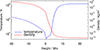 |
Fig. 1. Initial temperature and density stratification corresponding to the solar density and temperature stratification. The initial stratification only depends on the height z. |
We used periodic boundary conditions in the horizontal directions. At the bottom and top boundaries, we set the velocity to
 (7)
(7)
The setting uz = 0 prevents unwanted inflows of plasma in an undefined state. For simplicity, we used a constant solar luminosity at the bottom of our simulation domain to drive the convection. At the top of the box, we fixed the temperature to its initial value.
We employed Newton cooling to stabilize the photospheric and the chromospheric temperature stratification (Bourdin 2020). This scheme pushes the temperature gently back toward the initial stratification with a half-time τNC = 0.25 s of the exponential decay. Newton cooling helps to keep the lower atmosphere realistic because it would otherwise constantly loose energy through heat conduction. We did not model radiative transfer that would occur in semi-transparent denser layers of our model atmosphere, but Newton cooling mimics the effects of radiative transfer.
The initial 2D model atmosphere is only dependent on the z-coordinate, and it is hence identical to a collection of identical 1D stratifications. Without breaking this symmetry, our 2D simulation would evolve as multiple exactly replicated 1D models. Therefore, we added Gaussian noise to uz with a sigma of 131 m/s. The amplitude of the Gaussian noise was just large enough to break the symmetry while avoiding to introduce undesired effects. All our model runs used the same random seed for the generation of the Gaussian noise, which resulted in exactly the same initial conditions. This ensured comparability between all runs.
In the early evolution of the model, we used a velocity damping that was gradually faded out over the first 6000 s. This allowed the atmosphere to settle, to start the simulation smoothly, and to avoid the generation of disturbances that would eventually develop into shock waves. After the initial 6000 s, the system evolved freely.
All our model runs differed only in their viscosity schemes and coefficients. Therefore, the differences are not due to any other mechanisms or parameters.
We let the models run for a total of one solar day or until the simulation stopped for any reason, while the lifetime of a granule was only about 10 minutes. After about 50 life cycles of granules, we stopped the simulation because the convection slowly evolved into a state where the granular cells become too large and hence develop in an unrealistic way. The reason might be a too strong heat input from below. To track the temporal evolution, we wrote one snapshot every 20 s. Our parameter study comprised a total of 130 different settings (five sets with 26 runs per set).
We used three criteria to determine when the convection had fully formed: (1) The photosphere is fully covered by a pattern of alternating upward and downward motions, (2) more than half of the grid cells in the layer below the photosphere have upward motions, and (3) more than 90% of the convection cells reach an upward velocity of at least 400 m/s. We defined our formation time as the time at which these criteria were met. In addition, we determined the average size of a granule by dividing the horizontal extent of our model by the number of granules. At the same time, we also separately determined the vertical velocities as the root mean square values of the upward and downward motions.
3. Results
After the initial condition, our simulation evolved self-consistently. We describe here the general evolution of the reference run as a representation of the majority of the runs. The reference run developed the first signatures of the convection cells after 8000 s, and a granular vertical velocity pattern became visible on the surface. It took approximately another 2600 s until the entire surface was covered with granulation. Because of overshooting of the low-entropy plasma, the downdrafts from the intergranular lanes reached a depth of 3 Mm below the photosphere. Below this depth, the vertical velocities were low, and the granulation structure was lost. Separately, the heating from the bottom of the box produced separate convection cells with larger length scales and lower vertical velocities. The deep convection became visible after 9000 s had passed. For some time, two independent regions of convection were visible: The surface region, where the convection is driven by cooling at the surface, and the deep convection, where the heating causes the convective driving (Tschernitz & Bourdin 2025). Cooling as a driver for the surface convection was also indicated in simulations by Stein & Nordlund (2000).
Figure 2 shows three snapshots of the vertical velocities of the reference run at different times. The top panel shows the early evolution at a time of 3 h where two separate convection zones are present. The middle panel shows a fully evolved state at 4 h, where convective motions have spread to the previously unaffected region in between. After 5 h, the late phase of the simulation begins, where the granulation slowly became unstable. Between the deep and the surface convection, a gap with negligible velocities separates the two zones. In general, velocities are weaker in the bottom convection zone, while the spatial scale of the convection is larger. On the surface, the situation is reversed. In addition, the downdrafts have a smaller horizontal extent.
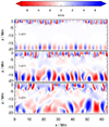 |
Fig. 2. Snapshots of the reference run at three different times. The top panel shows the run at the time when the surface is completely covered by granules. Convection at the bottom also develops, although there is still a region without significant convection between the two regions. The middle panel shows the same run one hour later, when the convection in both regions started to connect. The bottom panel shows the state of the simulation after the simulation advanced by another hour. The convection from below starts to destroy the surface granulation. Red shows a downward motion, and blue shows an upward motion. The color is saturated at ±7 km/s. |
With time, the extent of the regions increases until both zones merge, and convection is visible throughout the entire convection zone. This is shown in the lower panel in Fig. 2. After 27 000 s the pattern of convection slowly changes into a pattern of unrealistically large convection cells. The exact flow patterns are also highly time dependent, similar to what was reported by Hurlburt et al. (1984). We attribute this change to simplifications in our model. The heat input at the bottom is probably also too strong, causing a too strong driving of the deep convection, which eventually affects the surface convection in our model.
About three-quarters of our runs followed this general picture, although the timing might be different. The remaining quarter (32 runs) stopped between 7700 s and 9000 s, before our model photosphere was entirely covered with convection cells.
The main reason for failing runs was that the time step δt fell below the minimum criterion of δtmin = 10−6 s. From there, we did not to continue the computation because a numerical instability started to develop, and its resolution through diffusive terms in the equations, if possible at all, would require an infeasible amount of computing time. In these runs, very high peaks formed in either the temperature or the velocity, and sometimes in both. Localized temperature maxima became orders of magnitude hotter than usual coronal values. Peaking velocities, if not prevented, might even exceed the speed of light. These peaks are definitely a numerical issue caused by an insufficient diffusion term to treat extreme shear velocities or shocks in the model. Around high peaks, extreme gradients occur, which leads to a decrease in the time step due to the Courant criterion. A reduced lower limit for the time step did not help because the time step in these runs continued to drop.
All numerically stable runs produced at least 50 cycles of granulation or ran for at least 27 000 s of solar time. Hence, we categorized our runs that fully developed convection throughout the computational domain as ‘stable’ and the runs that stopped early due to numerical instabilities as ‘instable’.
For the parameter sets 1, 2, and 3, we obtained granules for all values of the kinematic viscosity. Sets 4 and 5 only produced convection for ν ≥ 1.34 ⋅ 107 m2/s, and the runs with lower ν are numerically not stable. The main difference was that in sets 1, 2, and 3 we kept the shock viscosity at a constant level. In set 4, the shock viscosity was scaled proportional to ν, and in set 5 no shock viscosity was applied. Therefore, the shock viscosity here is the key scheme to maintain numerical stability at lower kinematic viscosities because it provides the necessary viscosity even when the kinematic viscosity is too low for a given setup. Below νshock = 0.1, the shock viscosity is too low to provide a significant stabilizing effect, which led to numerical instability before the entire surface was covered with convection cells. This probably explains the asymptotic behavior for low values of ν together with a constant shock viscosity in sets 1, 2, and 3.
In Fig. 3, we compare the kinematic viscosity ν with the formation time for sets 1, 2, and 3. The convection formation times are similar, as is the same asymptotic behavior for small ν. In set 1, the formation time is roughly constant and asymptotic for ν < νcrit with νcrit = 1.34 ⋅ 107 m2/s. Above this critical value, the formation time increases significantly. For our highest ν, the formation time is about four times longer, which indicates the need of a stronger driving for higher viscosities. Granules emerge with unrealistically large spatial scales for solar granulation. Scaling the hyperviscosity together with the kinematic viscosity clearly does not change the formation time. When we compare sets 2 (scaled hyperviscosity) and 3 (no hyperviscosity), we see no significant differences. This shows that hyperviscosity does not play a significant role in our model.
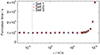 |
Fig. 3. Formation time of the photospheric granulation for sets 1, 2, and 3 vs. a varying kinematic viscosity ν. Runs with low kinematic viscosity have formation times around 10 000 s, while the time increases for runs with a higher kinematic viscosity. All three sets show a similar behavior. The dashed vertical line indicates the kinematic viscosity in the upper solar convection zone according to Miesch (2005). |
In Fig. 4, we compare the kinematic viscosity ν with the formation time in sets 1, 4, and 5. Except for the highest value of ν, the granulation in set 4 forms slightly earlier than in set 1 below ν = 1.34 ⋅ 108 m2/s and slightly later for values above ν = 1.34 ⋅ 108 m2/s.
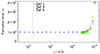 |
Fig. 4. Same plot as Fig. 3, but for sets 1, 4, and 5. Sets 4 and 5 do not develop convection below ν = 1.34 ⋅ 107 m2/s. Set 4 shows shorter formation times for runs when the scaled shock viscosity is below the value for the reference run and longer formation times for runs with a higher shock viscosity than the reference run. Set 5 shows generally shorter formation times, except for the run with the highest viscosity. |
Set 5 did not use any shock viscosity, and only runs with ν ≥ νcrit were numerically stable so that we might determine the formation time. For successful runs, the results of sets 1 and 5 are very similar. Below νcrit, the granulation formed slightly earlier in set 5.
Scaling the hyperviscosity together with the kinematic viscosity in set 4 did not change the formation time for the stable runs. Set 4 had no hyperviscosity, and the shock viscosity was scaled proportional to ν. Figure 4 shows that the shock viscosity is the key ingredient to make our runs numerically stable.
Without the shock viscosity (set 5), the formation of granules occurs slightly earlier than with the shock viscosity (sets 1 and 4). For set 4, the shock viscosity was increased in proportion to the kinematic viscosity and became higher than the reference value for ν > 1.34 ⋅ 108 m2/s, which led to a delayed formation of the granulation. In contrast to this, for ν < 1.34 ⋅ 108 m2/s the granulation formed earlier than with a constant shock viscosity because the total viscosity was lower and the plasma flowed more freely. When the kinematic viscosity reached ν = 1.34 ⋅ 1010 m2/s, the total viscosity was already so high that the plasma flow was strongly damped and shocks clearly did not appear. This shows that the shock viscosity has no significant effects for the highest ν value.
From this comparison, and in particular, from the instability of sets 4 and 5 for low kinematic viscosity, we learned that νcrit = 1.34 ⋅ 107 m2/s is our lower limit for the numerical feasibility of convection models with a proportionally scaled shock viscosity or without any shock viscosity. This result also depends on the grid distance Δx = 125 km of our model. At the same time, this value of νcrit is still close to the realistic asymptotic behavior of the runs with smaller viscosity coefficients. A more fine-grained test of slightly lower ν values before the next smaller scaling step was needed to approach the ideal choice of νcrit. As we already learned from set 4, a much smaller shock viscosity coefficient does not lead to numerical stability.
Figure 5 shows the variation in the length scale of the granules with the kinematic viscosity in our sets 1, 2, and 3. The formation time and the average diameter of the granules are roughly constant for kinematic viscosities of ν ≤ νcrit. In the asymptotic value range, the diameter fluctuated between 2.5 Mm and 3 Mm. This is significantly larger than the size of observed solar granules, whose average diameters are about 1.5 Mm (Bray & Loughhead 1977). The granule diameter increased strongly for ν > νcrit because the increased viscosity suppressed small-scale turbulence. The approximately constant diameter of the granules below the critical value might be due to the help of shock viscosity, which provides an effective additional viscosity.
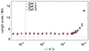 |
Fig. 5. Average diameter (spatial scale) of the photospheric granules vs. the kinematic viscosity ν for sets 1, 2, and 3. The dashed vertical gray line shows the realistic plasma viscosity in the upper convection zone. The dotted horizontal gray line roughly indicates the mean distance between the centers of two granules according to Bray & Loughhead (1977). |
No significant differences are visible in Fig. 6 between sets 1, 4, and 5. Again, the shock viscosity is needed for numerical stability of the runs with low kinematic viscosity. This means that below νcrit, our runs were instable. For high ν values, we found very large granule sizes because in these runs, the plasma was more restricted than in reality. The higher additional shock viscosity in set 4 than in set 5 might cause a higher total effective viscosity and the larger granulation diameter.
The vertical velocities have typical photospheric values of 0.5 to 0.9 km/s for upward velocities and 0.6 to 1.1 km/s for upward velocities (see Figs. 7 and 8). In the upper convection zone, these values reach up to ±7 km/s (see Fig. 2). The root mean square (RMS) of the vertical velocities differs by about 50% when we scaled ν. Figures 7 and 8 still show very similar vertical velocities for the same ν in sets 1, 4, and 5. For the highest tested ν value, which strongly suppressed the plasma motion, we find an expected decrease in both the upward and downward velocities. Moreover, for high ν values, there is an increasing effect on the downward velocities because the convection cells become larger, and hence, the downwards mass flux in the intergranular space needs to increase in order to compensate for all the upward mass flux from the larger granules. Since the density remains constant, as does the plasma pressure, the downflow velocity has to increase. We find similar trends in sets 2 and 3.
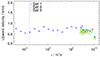 |
Fig. 7. Upward velocity component vs. the kinematic viscosity ν for sets 1, 4, and 5. The vertical dashed gray line represents the realistic value for the solar kinematic viscosity in the upper convection zone. |
4. Discussion
We investigated the effects of the kinematic viscosity, the hyperviscosity, and the shock viscosity using the Pencil Code with a 2D hydrodynamic convection setup. In a parameter study, we varied all viscosity coefficients over several orders of magnitude, and we combined the physical kinematic with purely numerical viscosity schemes. On the one hand, we found that the simulation runs that included a constant shock viscosity (sets 1, 2, and 3) are numerically stable enough to fully develop photospheric convection. On the other hand, sets 4 and 5 were numerically stable only for ν ≥ νcrit.
From the beginning, two separate regions with convective motions at the deep interior and at the surface existed. This can be explained by the entropy profile from the initial stratification of the solar interior. Our initial condition had a nearly flat entropy profile at the lower boundary with a slightly positive entropy gradient until close to the surface. The profile was calculated from the stratification in Fig. 1. It ranged from s/cp = 1.9 to s/cp = 3.2, while Barekat & Brandenburg (2014) used several different entropy profiles.
The entropy profile was calculated from the initial density and temperature stratification, which was taken from Table 2.4 in Stix (2002). The entropy gradient calculated from this stratification is negative only for the uppermost 4 Mm below the surface, indicating instability against convection. The rest of the convection zone in our simulation box had a positive gradient, indicating stability against convection. For the deep convection, we found instability against convection only deeper than 30 Mm below the surface. Convection can therefore start easily on the surface, where it is driven by the cooling of the material through radiative losses (Tschernitz & Bourdin 2025). The convection in the interior is driven by our heat input at the lower boundary, where it changes the entropy profile to become unstable against convection. Between these two convective regions, the velocities remain initially negligible. Finally, after about 7 hours, the entropy gradient becomes unstable in the entire convection zone in our simulation.
For kinematic viscosities above ν > νcrit, the granule diameter and the formation time of granules are strongly dependent on ν. Below this critical value νcrit, all key results, including the maximum vertical velocities, exhibit an asymptotic behavior.
Hence, the shock viscosity νshock stabilizes the simulation runs when the kinematic viscosity ν is too low to average out numerical instabilities. The shock viscosity scheme adds an additional diffusion term in regions with strong velocity gradients. Within our choice of parameters and viscosity schemes, hyperviscosity does not seem to have a significant effect on the granulation. Since the length scales and formation times in sets 1 and 2 are not significantly different, it is apparent that hyperviscosity is irrelevant for the large scales, which was intended for hyperviscosity schemes. At lower ν values, the constant shock viscosity is the main reason for numerical stability, and we did not find significant effects from the hyperviscosity.
For ν < νcrit, the runs did not produce numerically stable convection unless a sufficient shock viscosity was present as well. Moreover, our granulation results did not depend on ν for ν < νcrit. As our steps are about factors of 5, this critical value is a rough estimate and not an exact value.
The question now is why a kinematic viscosity of about 107 m2/s is critical regarding the stability of a run. Explicit numerical schemes, even together with high-order derivatives, cannot deal with grid Reynolds numbers much larger than unity. The grid Reynolds number is defined as
 (8)
(8)
with the grid distance Δx as the typical length scale, and v as the absolute value of the local velocity, which equals the ratio of the advective forces Fadvec and the diffusive forces Fdiffus. From experience and from the manual, we know that the Pencil Code can deal with grid Reynolds numbers larger than 5 only for a short time.
In our runs, we achieved grid Reynolds numbers of up to 10 for the critical kinematic viscosity coefficient νcrit. Therefore, we even exceeded the critical grid Reynolds number in small regions and for short times. The other viscosity schemes (here, the shock viscosity) enhance the viscous force in these critical regions, and this alone decreases the effective grid Reynolds number and the run stays numerically stable.
If we had not applied an additional shock viscosity, the runs would have become unstable for low kinematic viscosity ν because the grid Reynolds number increases as Rgrid ∼ 1/ν. Therefore, lower viscosities induce higher grid Reynolds numbers, which then rise above the limit of what our code can handle numerically.
We explain the delayed formation of the granulation due to a higher kinematic viscosity with the fact that higher viscous forces require higher driving forces to achieve the same goal. A similar behavior was found in Barekat & Brandenburg (2014), where the Rayleigh number was a control parameter for the onset of convection. Since our convectional driving was the same in all runs, the very viscous media simply need more time to fully form all convection cells. The hyperviscosity does not have a discernible influence on the formation time.
In our set 5, the convection started slightly earlier than in all other sets. A possible explanation is that we only used the kinematic viscosity in set 5. Without the contribution of the other viscosity schemes, there is less resistance for the fluid motion, and the convection may start more easily.
For the highest value of ν, the formation time was the same in all sets because the kinematic viscosity was so high that it was the predominant viscous force on the fluid motion. The only exception was set 4, where the shock viscosity was proportional to ν and therefore even increased the already strong kinematic viscosity. The total viscosity was highest in set 4 for ν > νcrit compared to all other sets, and it thus led to the longest times of granulation formation.
Higher kinematic viscosities also lead to larger granules for ν > νcrit. This is expected because overly strong viscosity suppresses small-scale turbulence and leads to larger structures. The granule size was roughly constant for ν ≤ νcrit, and we explain this asymptotic behavior again with the dominance of the constant shock viscosity in sets 1, 2, and 3 for low ν. Without the shock viscosity, we would require a kinematic viscosity that is higher than the realistic solar value by about eight orders of magnitude for our grid distances of Δx = 125 km.
Finally, our granules are larger by about 40% than the real ones on the Sun. A more realistic size might be achieved by adjusting the different viscosity coefficients and maybe even adjusting the grid distance to lower values. The ionization equilibrium, radiative transfer, and the polytropic index of the plasma also play a role. Furthermore, our runs lacked the third spatial dimension, which gives a higher degree of freedom to the plasma motion on the real Sun.
The velocities of upflows and downflows also show this asymptotic behavior for ν < νcrit. Together with changing granule sizes for higher ν, we also expect different plasma flow velocities. Larger granules with roughly the same upflow velocity accumulate more mass coming to the photosphere. Because the intergranular area remains roughly constant, these regions have to compensate for the upward mass flux with enhanced downflow velocities. This trend is visible in the results of runs with high ν, except for the highest ν values, where both upflows and downflows are suppressed by the strong viscous force.
In the later evolution of our model, after about half a solar day, the convection cells became larger and more closely resembled one large cell that spanned the whole box. Barekat & Brandenburg (2014) also observed a similar effect. Their setup switched from a multicell convection to a single-cell configuration over time. The authors speculate that this might be a consequence of their setup, in particular, the entropy influx from below or the photospheric radiative cooling, which both might drive the convection too strongly. Hurlburt et al. (1984) found in their early models that convection is time dependent for aspect ratios equal to or lower than 3, where no steady solution developed.
To investigate these puzzling earlier results, we performed our reference run from set 1 with a simulation domain of twice the horizontal extent, so that we achieved an aspect ratio well above 3 for the convection zone. Although the size of the photospheric granules still increased with time, a granulation pattern was still visible at later times, when this pattern was no longer visible in models with a lower aspect ratio. This shows that the aspect ratio is another important parameter.
Although we used realistic temperature and density stratifications, we still missed ionization effects within the upper convection zone and up to the transition region. Even though we used some approximate mechanisms instead of a full radiative transfer treatment in the photosphere and up to the transition region, some differences from reality still remain. Moreover, we did not take any spherical or rotational effects into account that act on the real Sun. The lack of magnetic fields in our model is justified by the fact that plasma beta in the upper convection zone is usually higher than unity. Despite these shortcomings, our model results are still comparable to realistic parameters of solar granulation.
Future work might estimate the numerical viscosity in models similar to ours with many runs, where each runs would have a different realization of the fluctuations in the initial condition. We strongly recommend always to use an explicit viscosity that is higher by orders of magnitude than the numerical viscosity because the latter is not physically motivated.
5. Conclusions
We found that kinematic viscosity should be combined with other schemes that improve numerical stability around extreme velocity gradients, such as a shock-viscosity scheme. We found that this allowed us to scale the kinematic viscosity down and still maintain numerical stability in our 2.5-dimensional hydrodynamic model of the upper solar convection zone and lower atmosphere.
The shock viscosity has a stabilizing effect that keeps the grid Reynolds number below a certain numerically critical value in our high-order explicit solver for partial differential equations. We conclude that the shock viscosity causes the asymptotic behavior of various granulation characteristics for a kinematic viscosity below the critical limit ν < νcrit. We therefore recommend using a shock viscosity scheme together with the kinematic viscosity. Hyperviscosity is not recommended because it is a purely numerical scheme to dissipate energy at small scales and to deal with wiggles. Therefore, this scheme ought to be avoided, especially as it cannot be guaranteed that it is convergent with regular dissipation. Our simulations clearly showed that hyperviscosity has little effect on the simulations compared to shock viscosity.
The question then is why a kinematic viscosity is needed at all. Some of our runs showed wiggles (spurious oscillations of a quantity that are a purely numerical effect due to insufficient diffusion) in the convection zone when the kinematic viscosity was too low. The kinematic viscosity acts everywhere and does indeed have a physical counterpart even in almost collisionless plasmas. The shock viscosity acts only where strong velocity gradients (including shear velocities) would trigger an additional diffusion. For realistic simulations, the kinematic viscosity should therefore still be employed, with a value as low as permitted by the classical dilemma between numerical needs and physical realism.
When the kinematic viscosity is set too low, the grid Reynolds number increases, and this can cause wiggles in the vertical component of the plasma velocity within the convection zone in locations with strong vertical shear motions. The reason for this is a lack of diffusion to smooth out small numeric inaccuracies, which allows these errors to amplify over time. It is also important to set the kinematic viscosity according to the grid distance. When the kinematic viscosities are too high, they would suppress the desired turbulent motions, and this would lead to spurious effects in the convection, such as oversized granules.
We recommend scaling the viscosity according to the grid size, with a recommended value of νcrit = 1.34 ⋅ 107 m2/s for a grid distance of Δx = 125 km. In case of strong shear flows, which are present at the boundary between granules and intergranular lanes, an additional shock viscosity can provide increased numerical stability. For the Pencil Code, we recommend values between 0.1 and 1 of the dimensionless scaling parameter. A different grid scale will require different values for the kinematic and shock viscosity, but the question whether the value must be scaled proportional or inversely proportional cannot be answered in this study. Pandey & Bourdin (2025) have shown that an inversely proportional (and hence counterintuitive) scaling of the diffusivities may be required for a stable numerical model.
Acknowledgments
This research was funded in whole or in part by the Austrian Science Fund (FWF) [10.55776/P32958] and [10.55776/P37265]. For open access purposes, the author has applied a CC BY public copyright license to any author-accepted manuscript version arising from this submission.
References
- Barekat, A., & Brandenburg, A. 2014, A&A, 571, A68 [NASA ADS] [CrossRef] [EDP Sciences] [Google Scholar]
- Bourdin, P. A. 2014, Cent. Eur. Astrophys. Bull., 38, 1 [Google Scholar]
- Bourdin, P.-A. 2020, Geophys. Astrophys. Fluid Dyn., 114, 235 [NASA ADS] [CrossRef] [Google Scholar]
- Bray, R. J., & Loughhead, R. E. 1977, Sol. Phys., 54, 319 [Google Scholar]
- Cartier-Michaud, T., Ghendrih, P., Sarazin, Y., et al. 2016, Phys. Plasmas, 23, 020702 [NASA ADS] [CrossRef] [Google Scholar]
- Cossette, J.-F., Charbonneau, P., Smolarkiewicz, P. K., & Rast, M. P. 2017, ApJ, 841, 65 [CrossRef] [Google Scholar]
- Fontenla, J. M., Avrett, E. H., & Loeser, R. 1990, ApJ, 355, 700 [NASA ADS] [CrossRef] [Google Scholar]
- Gizon, L., & Birch, A. C. 2005, Liv. Rev. Sol. Phys., 2, 6 [Google Scholar]
- Gray, D. F., & Nagel, T. 1989, ApJ, 341, 421 [NASA ADS] [CrossRef] [Google Scholar]
- Haugen, N. E. L., & Brandenburg, A. 2004, Phys. Rev. E, 70, 026405 [Google Scholar]
- Hotta, H., & Kusano, K. 2021, Nat. Astron., 5, 1100 [NASA ADS] [CrossRef] [Google Scholar]
- Hotta, H., Iijima, H., & Kusano, K. 2019, Sci. Adv., 5, 2307 [Google Scholar]
- Hurlburt, N. E., Toomre, J., & Massaguer, J. M. 1984, ApJ, 282, 557 [NASA ADS] [CrossRef] [Google Scholar]
- Käpylä, P. J., Mantere, M. J., Cole, E., Warnecke, J., & Brandenburg, A. 2013, ApJ, 778, 41 [CrossRef] [Google Scholar]
- Kupka, F., & Muthsam, H. J. 2017, Liv. Rev. Comput. Astrophys., 3, 1 [Google Scholar]
- Laney, C. B. 1998, Computational Gasdynamics (Cambridge University Press) [Google Scholar]
- Margolin, L. G. 2019, Shock Waves, 29, 27 [NASA ADS] [CrossRef] [Google Scholar]
- Miesch, M. S. 2005, Liv. Rev. Sol. Phys., 2, 1 [Google Scholar]
- Nelson, N. J., Featherstone, N. A., Miesch, M. S., & Toomre, J. 2018, ApJ, 859, 117 [Google Scholar]
- November, L. J., & Koutchmy, S. 1996, ApJ, 466, 512 [CrossRef] [Google Scholar]
- Pandey, V., & Bourdin, P.-A. 2025, A&A, 693, A89 [NASA ADS] [CrossRef] [EDP Sciences] [Google Scholar]
- Pencil Code Collaboration (Brandenburg, A., et al.) 2021, J. Open Source Softw., 6, 2807 [Google Scholar]
- Pope, S. B. 2000, Turbulent Flows (Cambridge University Press) [Google Scholar]
- Riva, F., & Steiner, O. 2022, A&A, 660, A115 [NASA ADS] [CrossRef] [EDP Sciences] [Google Scholar]
- Smolarkiewicz, P. K., & Margolin, L. G. 1998, J. Comput. Phys., 140, 459 [Google Scholar]
- Stein, R. F., & Nordlund, Å. 2000, Sol. Phys., 192, 91 [NASA ADS] [CrossRef] [Google Scholar]
- Stein, R. F., Nordlund, Å., Collet, R., & Trampedach, R. 2024, ApJ, 970, 24 [NASA ADS] [CrossRef] [Google Scholar]
- Stix, M. 2002, The Sun: An Introduction (Berlin Heidelberg GmbH: Springer-Verlag) [Google Scholar]
- Tschernitz, J., & Bourdin, P.-A. 2025, ApJ, 979, L39 [Google Scholar]
- Vögler, A., & Schüssler, M. 2007, A&A, 465, L43 [Google Scholar]
All Tables
All Figures
|
Fig. 1. Initial temperature and density stratification corresponding to the solar density and temperature stratification. The initial stratification only depends on the height z. |
| In the text | |
|
Fig. 2. Snapshots of the reference run at three different times. The top panel shows the run at the time when the surface is completely covered by granules. Convection at the bottom also develops, although there is still a region without significant convection between the two regions. The middle panel shows the same run one hour later, when the convection in both regions started to connect. The bottom panel shows the state of the simulation after the simulation advanced by another hour. The convection from below starts to destroy the surface granulation. Red shows a downward motion, and blue shows an upward motion. The color is saturated at ±7 km/s. |
| In the text | |
|
Fig. 3. Formation time of the photospheric granulation for sets 1, 2, and 3 vs. a varying kinematic viscosity ν. Runs with low kinematic viscosity have formation times around 10 000 s, while the time increases for runs with a higher kinematic viscosity. All three sets show a similar behavior. The dashed vertical line indicates the kinematic viscosity in the upper solar convection zone according to Miesch (2005). |
| In the text | |
|
Fig. 4. Same plot as Fig. 3, but for sets 1, 4, and 5. Sets 4 and 5 do not develop convection below ν = 1.34 ⋅ 107 m2/s. Set 4 shows shorter formation times for runs when the scaled shock viscosity is below the value for the reference run and longer formation times for runs with a higher shock viscosity than the reference run. Set 5 shows generally shorter formation times, except for the run with the highest viscosity. |
| In the text | |
|
Fig. 5. Average diameter (spatial scale) of the photospheric granules vs. the kinematic viscosity ν for sets 1, 2, and 3. The dashed vertical gray line shows the realistic plasma viscosity in the upper convection zone. The dotted horizontal gray line roughly indicates the mean distance between the centers of two granules according to Bray & Loughhead (1977). |
| In the text | |
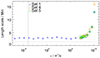 |
Fig. 6. Same plot as Fig. 5, but for sets 1, 4, and 5. |
| In the text | |
|
Fig. 7. Upward velocity component vs. the kinematic viscosity ν for sets 1, 4, and 5. The vertical dashed gray line represents the realistic value for the solar kinematic viscosity in the upper convection zone. |
| In the text | |
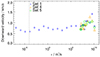 |
Fig. 8. Same as Fig. 7, but showing the downward velocity component. |
| In the text | |
Current usage metrics show cumulative count of Article Views (full-text article views including HTML views, PDF and ePub downloads, according to the available data) and Abstracts Views on Vision4Press platform.
Data correspond to usage on the plateform after 2015. The current usage metrics is available 48-96 hours after online publication and is updated daily on week days.
Initial download of the metrics may take a while.