| Issue |
A&A
Volume 701, September 2025
|
|
|---|---|---|
| Article Number | A5 | |
| Number of page(s) | 13 | |
| Section | Stellar structure and evolution | |
| DOI | https://doi.org/10.1051/0004-6361/202452885 | |
| Published online | 01 September 2025 | |
Interior rotation modelling of the β Cep pulsator HD 192575 including multiplet asymmetries
1
Institute of Astronomy, KU Leuven, Celestijnenlaan 200D, 3001 Leuven, Belgium
2
School of Mathematics, Statistics and Physics, Newcastle University, Newcastle upon Tyne, NE1 7RU, UK
3
Institute of Science and Technology Austria (ISTA), Am Campus 1, Klosterneuburg, Austria
4
Center for Astrophysics | Harvard & Smithsonian, 60 Garden Street, Cambridge, MA, 02138, USA
5
Université Paris-Saclay, Université Paris Cité, CEA, CNRS, AIM, 91191 Gif-sur-Yvette, France
6
Department of Astrophysics, IMAPP, Radboud University Nijmegen, PO Box 9010 6500 GL Nijmegen, The Netherlands
7
Max Planck Institute for Astronomy, Königstuhl 17, 69117 Heidelberg, Germany
⋆ Corresponding author: This email address is being protected from spambots. You need JavaScript enabled to view it.
Received:
5
November
2024
Accepted:
9
July
2025
Abstract
Context. Rotation plays an important role in stellar evolution. However, the mechanisms behind the transport of angular momentum in stars at various stages of their evolution are not well understood. To improve our understanding of these processes, it is necessary to measure and validate the internal rotation profiles of stars across different stages of evolution and mass regimes.
Aims. Our aim is to constrain the internal rotation profile of the 12-M⊙ β Cep pulsator HD 192575 from the observed pulsational multiplets and the asymmetries of their component frequencies.
Methods. We updated the forward asteroseismic modelling of HD 192575 based on new TESS observations. We inverted the rotation profile from the symmetric part of the splittings and computed the multiplet asymmetries due to the Coriolis force and stellar deformation, which we treated perturbatively. We compared the computed asymmetries with the observed asymmetries.
Results. Our new forward asteroseismic modelling is in agreement with previous results but with increased uncertainties, partially due to increased frequency precision, which required us to relax certain constraints. Ambiguity in the mode identification is the main source of the uncertainty, which also affects the inferred rotation profiles. Almost all acceptable rotation profiles occur in the regime below 0.4 d−1 and favour weak radial differential rotation, with a ratio of core to envelope rotation of less than 2. We find that the quality of the match between the observed and theoretically predicted mode asymmetries is strongly dependent on the mode identification and the internal structure of the star.
Conclusions. Our results offer the first detailed rotation inversion for a β Cep pulsator. They show that the rotation profile and the mode asymmetries provide a valuable tool for further constraining the evolutionary properties of HD 192575, and in particular the details of angular momentum transport in massive stars.
Key words: asteroseismology / magnetic fields / stars: interiors / stars: magnetic field / stars: oscillations / stars: rotation
© The Authors 2025
 Open Access article, published by EDP Sciences, under the terms of the Creative Commons Attribution License (https://creativecommons.org/licenses/by/4.0), which permits unrestricted use, distribution, and reproduction in any medium, provided the original work is properly cited.
This article is published in open access under the Subscribe to Open model. This email address is being protected from spambots. You need JavaScript enabled to view it. to support open access publication.
1. Introduction
The transport of angular momentum in stars with a convective core as measured through asteroseismology does not align with theoretical predictions for a significant number of stars (Eggenberger et al. 2012; Marques et al. 2013; Goupil et al. 2013; Ceillier et al. 2013; Cantiello et al. 2014; Fuller et al. 2014; Belkacem et al. 2015; Ouazzani et al. 2019; Moyano et al. 2022; Salmon et al. 2022; Bétrisey et al. 2023); see Aerts et al. (2019) for a review. Various mechanisms such as magnetic fields (e.g. Mestel & Weiss 1987; Spruit 2002; Mathis & Zahn 2005; Fuller et al. 2019; Takahashi & Langer 2021) and internal gravity waves (e.g. Schatzman 1993; Zahn et al. 1997; Talon et al. 2002; Rogers et al. 2013; Fuller et al. 2014; Rogers 2015) are proposed as possible solutions to this inconsistency. In order to validate such proposals, it is necessary to measure the rotation profile of stars at various masses and stages of evolution. However, the internal rotation profiles of only a handful of massive stars have been constrained from their oscillation frequencies (Bowman 2020).
The β Cep star HD 192575 discovered in Transiting Exoplanet Survey Satellite (TESS; Ricker et al. 2014) space photometry is a unique calibrator for interior rotation (Burssens et al. 2023). While studies of β Cep stars go back more than a century (see the reviews by Sterken & Jerzykiewicz 1993; Aerts & De Cat 2003; Stankov & Handler 2005; Bowman 2020), few such stars have been modelled asteroseismically, and fewer still have a reliable measurement of their internal rotation rates (Aerts et al. 2003; Pamyatnykh et al. 2004; Dupret et al. 2004; Briquet et al. 2007; Dziembowski & Pamyatnykh 2008; Suárez et al. 2009; Salmon et al. 2022). HD 192575 was modelled asteroseismically by Burssens et al. (2023) based on the detection of rotationally split multiplets of low-order pressure (p) and gravity (g) modes in its frequency spectrum deduced from 352 d of cycle 2 TESS space photometry. Three of these multiplets, two g-mode and one p-mode multiplet, were used in the subsequent forward asteroseismic modelling. HD 192575 was found to be a differentially rotating star with a mass of  M⊙ approaching the end of its main-sequence life with a central hydrogen mass fraction of
 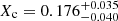 .
.
Internal rotation profiles of slowly rotating stars have been derived from the symmetric component of rotationally split multiplets (e.g. Deheuvels et al. 2012, 2014; Kurtz et al. 2014; Di Mauro et al. 2016, 2018; Triana et al. 2015, 2017; Hatta et al. 2019, 2022; Aerts & Tkachenko 2024), but moderate-to-fast rotation also causes asymmetrical splittings (Saio 1981; Gough & Thompson 1990; Soufi et al. 1998; Suárez et al. 2006). Other effects also contribute to these asymmetries, such as the presence of a magnetic field (e.g. Gough & Thompson 1990; Mathis et al. 2021; Bugnet et al. 2021; Loi 2021; Li et al. 2022; Bugnet 2022; Mathis & Bugnet 2023; Bharati Das et al. 2024; Guo et al. 2024; Bhattacharya et al. 2024), which has been used to derive the internal magnetic field strengths of red giants (Li et al. 2022; Deheuvels et al. 2023). Characterising the effect of rotation on the asymmetries, and validating the consistency of the observed asymmetries with these theoretical predictions, is useful for both constraining the rotation profile and providing a starting point for further investigation into these additional contributions. Thus far, only the asymmetries of two β Cep stars, ν Eri and θ Oph, have been analysed in detail (Pamyatnykh et al. 2004; Briquet et al. 2007; Suárez et al. 2009).
We aim to derive the internal rotation profile of HD 192575 from its observed multiplet splittings and investigate whether the theoretical asymmetries match the observed ones, given the new rotation profile. First, we determined the internal rotation profile from the symmetric part of the splittings of HD 192575 using more recently available TESS data (i.e. cycles 2 and 4; Sect. 2) via rotation inversion (Sect. 3). Using the candidate rotation profiles, we computed rotational asymmetries for the modelled modes based on a perturbative approach (Sect. 4). These asymmetries were then compared to the observed asymmetries to check whether they are consistent. We summarise our results and conclude in Sect. 5.
2. New asteroseismic modelling
HD 192575 is an early-B dwarf that continues to be observed by TESS in its northern continuous viewing zone. It has a rich frequency spectrum with multiple g- and p-mode rotationally split multiplets, with frequencies ranging from 3.5 d−1 to 15 d−1. One of the features of this frequency spectrum is the overlap of two multiplets in the g-mode dominated regime between 3.5 d−1 and 4.5 d−1 cycles per day (we refer to these as quint1a and quint1b; see Fig. 1). Burssens et al. (2023) identified these as two ℓ = 2 multiplets, and therefore they must be adjacent in radial order, and by necessity undergoing an avoided crossing with each other. This was used by Burssens et al. (2023) to constrain the properties of HD 192575.
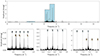 |
Fig. 1. Frequency spectrum of HD 192575. Top panel: Full frequency spectrum, with the regions with fitted modes indicated by the light blue boxes. Bottom panels: Zoomed-in views of those boxes. From left to right, the multiplets are given the names quint1a (blue, first panel), quint1b (orange, first panel), quad1 (blue, second panel), trip1 (blue, third panel), and trip2 (orange, third panel). |
We have updated this modelling because TESS revisited HD 192575 during its extended mission, yielding new light curves and therefore revised oscillation frequencies and mode identifications. The results of these new modelling efforts can be found in Table 1. We used the same grid of Modules for Experiments in Stellar Astrophysics (MESA; Paxton et al. 2011, 2013, 2015; Paxton et al. 2018, 2019; Jermyn et al. 2023) and GYRE (Townsend & Teitler 2013; Townsend et al. 2018; Goldstein & Townsend 2020) models and the same modelling techniques and software as Burssens et al. (2023). The only difference, as explained below, between our work and the work of Burssens et al. (2023) is the updated observed mode frequencies and the mode identification based on new TESS data.
Best model parameters and 2σ confidence intervals for the forward asteroseismic modelling of HD 192575 for the original modelling by Burssens et al. (2023) and our seven new modelling sets.
At the time of the asteroseismic modelling of HD 192575 by Burssens et al. (2023), only cycle 2 of TESS observations was available. Meanwhile, TESS has revisited HD 192575 during its extended mission. We combined all the available TESS data for this star until the end of 2023. We extracted the 2-min cadence Pre-search Data Conditioning Simple Aperture Photometry light curves from MAST1, applied the same reduction and detrending routines as Burssens et al. (2023), and reanalysed them using the iterative pre-whitening routines of Bowman & Michielsen (2021). The pulsation mode frequencies extracted for the g-mode and p-mode multiplets based on the combined cycles 2 and 4 TESS light curves are listed in Appendix A.
Due to the extended time base of the combined cycles 2 and 4 TESS light curve, some pulsation mode frequencies, which previously were unresolved or statistically insignificant compared to the noise in the frequency spectrum, are now identified as significant. This includes an additional mode in the quint1a multiplet, requiring a different assignment of the azimuthal orders compared to the identification by Burssens et al. (2023). The zonal mode of this multiplet is now set at the 3.84 d−1 mode instead of the 3.64 d−1 mode (see Fig. 1).
In their work, Burssens et al. (2023) limited the selection of valid models by enforcing an avoided crossing criterion, meaning that the frequency difference between the two identified g-mode multiplets should be similar to the observed frequency difference, allowing for observational uncertainties. With the extended time base of the TESS observations, this observed difference has decreased by about a factor of 2. Therefore, we reapplied the same forward asteroseismic modelling framework for HD 192575 with these stricter constraints. We find that the radial orders of the modes increase by unity, that is, the ℓ = 2 g2, g1, and p2 modes are now identified as g1, f, and p3, respectively. Using the same constraints on effective temperature and luminosity derived by Burssens et al. (2023), a spectroscopic selection criterion using 2σ confidence intervals in the Hertzsprung–Russell diagram, only 7 structure models in the grid of MESA models provide appropriate matches of predicted frequencies that fit the TESS data. In order to maintain a reasonably wide sample of forward models, we relaxed the spectroscopic confidence intervals to 3σ, with 42 MESA structure models surviving this cut. As was done by Burssens et al. (2023), we implemented a cutoff for low Xc, keeping only models with Xc ≥ 0.05, to drop outliers before computing the confidence intervals. These evolved models are separated in the Hertzsprung–Russell diagram from the other models and have a much lower likelihood (about one to two orders of magnitude) than the best fitting models, but would skew the confidence intervals in Table 1 significantly. Additionally, they have a lower probability of being observed, owing to the short-lived contraction phase near the terminal-age main sequence. The resulting 2σ confidence intervals on the structure parameters, such as mass and age, are similar to the original modelling results of Burssens et al. (2023). Thus, the results of the forward asteroseismic modelling in this work are comparable to those performed previously, meaning they are not so sensitive to the updated mode identification. In the remainder of this paper we refer to this new set of best-fitting forward models as the ‘new-frequencies’ model set.
We now consider alternative explanations for the two close g-mode multiplets, as this is the most constraining factor in the forward asteroseismic modelling. For example, one of the multiplets could be a higher angular degree multiplet (e.g. ℓ = 3, ℓ = 4) that purely by chance ended up in a similar frequency location, and with similar splittings. Another possibility is that there is only one multiplet, but it is split by both rotation and a misaligned magnetic field (e.g. Loi 2021). We allowed for these possibilities by fitting only one of the two g-mode multiplets. Due to the proximity of these multiplets, the choice of which multiplet to keep, and which multiplet to discard, does not affect our use case. We present and used the result for the forward asteroseismic modelling with the quint1a multiplet, ignoring the quint1b multiplet. Furthermore, we attempted to fit three of the higher-frequency observed multiplets: the quadruplet already fitted by Burssens et al. (2023, quad1), the triplet containing the dominant mode (trip1), and one more triplet (trip2). These selections were made based on an initial fit of only quint1a and trip1, and we assumed that quint1a is an l = 2 mode and trip1 is an l = 1 mode.
With the constraint from the avoided crossing between the g-mode multiplets removed, multiple sets of mode identifications are possible. We constrained the mode degrees to ℓ = 1 and ℓ = 2 as none of the multiplets consist of more than five frequencies, and higher-degree modes are less likely to be observed due to geometric cancellation effects. Once the mode identifications of quint1a and trip1 are fixed, the other modes (quad1 and trip2) are also fixed, as only the frequencies of a handful of radial orders fall in the region with the observed multiplets. We find that quad1 and trip2 should both be ℓ = 2 modes, with adjacent radial orders.
We selected six sets of mode identifications that fit the observed frequencies best. All mode identifications used can be found in Table 2. Confidence intervals are provided in Table 1 for the associated parameters. It is worth noting that there are multiple candidates in the quad1 and trip2 multiplet for the zonal mode, and that different choices for the zonal mode do not yield the exact same forward modelling results. However, the variation introduced by this freedom is smaller than the variation between the different mode identifications of the multiplets. Hence, we only considered one choice for the zonal mode, which is given in Table A.1.
Mode identification of the multiplets used for the different model sets, given as (ℓ,npg).
Compared to the restricted modelling results, the central hydrogen fraction, Xc, for these six model sets is less constrained, as we no longer rely on the constraining power of the avoided crossing (see Table 1). This also generally increases the confidence intervals of all the inferred parameters, such as the convective core mass. The estimated model parameters are almost identical among the different sets of models. The initial stellar mass ranges from 10.5 M⊙ to 13.5 M⊙ for all but one of the model sets, while the metallicity and the convective boundary mixing (CBM) parameter, fCBM, are effectively unconstrained, spanning the entire parameter space, which was also reported by Burssens et al. (2023) owing to inherent model parameter degeneracies. It is important to note that the 2σ confidence intervals quoted in Table 1 do not take into account the different correlation structures across the different model sets. While we cannot compare the likelihood of sets 1 to 6 with the ‘original’ and new-frequencies model sets, as they use different observed quantities, it is possible to compare sets 1 to 6 amongst themselves.
Models close to the end of the main sequence are less likely to be observed from a evolutionary timescale standpoint. The further along its main-sequence life the star is, the faster it burns the remaining hydrogen in its core. The main sequence is followed by a fast contraction phase, where a significant fraction of energy is generated by gravitational collapse whilst a small fraction of hydrogen remains in the core. Hence, stars with lower Xc should be observed less likely in nature. This effect was not directly taken into account by Burssens et al. (2023) when computing the likelihood of a certain stellar model. Therefore, our modelling also does not take this effect into account, as we used the same modelling strategy as Burssens et al. (2023) to be able to compare our results. Figure 2 shows the probability density function of observing one of our evolutionary tracks as afunction of Xc. In the range given by our models, the likelihood of finding the star changes approximately by a factor of 2, which is another factor of 2 less likely compared to a star close to the zero-age main sequence. While low Xc are less likely, thedifference is not so large as to completely discredit models at Xc close to zero. This effect of timescales would be most relevant for the selection of the best model for each of the model sets, especially for model sets 4 through 6.
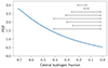 |
Fig. 2. Probability density function of observing one of the models at a certain central hydrogen fraction. The intervals (black) show the uncertainty regions for the central hydrogen fraction for each of the model sets (see Table 1). From top to bottom, the intervals show the original, new-frequencies, and sets 1 through 6 solutions. |
From a population viewpoint, β Cep stars with Xc < 0.1 can be considered outliers (who used the same model grid as we do Fritzewski et al. 2025). All of the model sets have solutions within this region, and it would be reasonable to consider such solutions as less likely. Similar to the timescale effect from the previous paragraph, we did not include the population in the forward modelling, to remain consistent with Burssens et al. (2023).
3. Rotation inversion
3.1. Setup
In this section we infer the rotation profile of HD 192575 from the observed multiplets. We used the symmetric part (the average of all splittings) of these multiplets as input for the rotation inversion, as the asymmetric components depend on the rotation frequency only at the second or higher order. The uncertainties on these symmetric components include both the uncertainty on the observed mode frequencies and the range of splittings for each multiplet, taken as a 1σ uncertainty. This second effect is dominant, as the observational uncertainties are of the order of 10−6 d−1, while the asymmetries are of the order of 10−3 d−1. For each of the model sets discussed in Sect. 2, we considered the 100 best-fitting models, except for the new-frequencies model set, as it only contains 42 models within the 3σ confidence intervals for effective temperature and luminosity.
As in Burssens et al. (2023), we used the Mahalanobis distance (Mahalanobis 1936) with an additional term for the theoretical variance of the stellar models as merit function (Aerts et al. 2018). Some models appear in multiple model sets, but the inferred rotation profiles are distinct, as the mode identification for each model set is different.
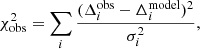
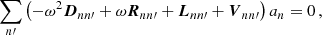
We performed a regularised least-squares (RLS) fit (e.g. Christensen-Dalsgaard et al. 1990) for each of the models to derive the internal rotation profile of HD 192575. RLS fit is a linear least-squares fit, with an additional penalty term for non-regular profiles. This penalty term is multiplied by a regularisation parameter to balance the importance of the observations and the level of regularity. We fitted the same frequencies with the same associated mode identifications as those used in the forward asteroseismic modelling in Sect. 2. The basis functions are degree two b-splines with 14 knots, which are equally spaced from the centre of the star to the surface, except for the endpoints (i.e. the centre of the star and the surface), where three knots are placed at the same location. This is to ensure that the resulting spline basis functions are localised and do not gain large tails near the edges of the interval. This gives us a total of 11 control points, which are free parameters in the fit. The rotation profile is regularised by the norm of its first derivative, which is integrated over the entire star. We varied the regularisation parameter such that we adequately covered the range around a χobs2 error of unity, therefore allowing for potentially under- and over-fitting. The χobs2 error includes only the observational errors, and not the contribution from the regularisation in the optimisation:
 (1)
(1)
where Δiobs and Δimodel are the observed and modelled multiplet splittings, and σi are the uncertainties on these splittings, which include the range spanned by the asymmetries.
To select the final rotation profiles, we used two criteria: (i) the L-curve criterion (Hansen 2001) and (ii) the rotation profiles reproduce the observed splittings. The L-curve is a log-log plot comparing the goodness of fit, given by χobs2, and how much the profile deviates from a ‘regular’ profile, as defined by the regularisation condition. It can help determine optimal values for the regularisation parameter by looking for parts of the diagram that have a similar shape as the letter L. The value of the regularisation parameter that results in the point in the corner would then be the optimal value (Hansen 2001). For this second criterion, we took the rotation profile with the largest regularisation parameter that still has the splittings within the observed uncertainty region. We used this method instead of more commonly used point measures such as the optimally localised averages family of methods (e.g. Pijpers & Thompson 1994) since we needed a full rotation profile from the centre to the surface of the star to be able to compute mode asymmetries (see the next section).
Apart from constructing rotation profiles to understand the asymmetry of the multiplets, we also compared our results with the results from forward asteroseismic modelling performed by Burssens et al. (2023) and with the rotation profiles computed by Mombarg et al. (2023) using the 2D stellar structure and evolution code ESTER (Espinosa Lara & Rieutord 2013; Mombarg et al. 2023). Burssens et al. (2023) considered only monotonic rotation profiles, consisting of a core rotation rate, a surface rotation rate, with a transition region between the two. They considered multiple permutations for the location and extent of this transition region: (i) the region where CBM takes place; (ii) the region where a gradient exists in the mean molecular weight (μ) left behind by the receding core; and (iii) the entire envelope. In each case, the core was found to be rotating faster than the surface by at least a factor of 1.2 and up to factor of 12.8, including observational uncertainties and uncertainties on the forward asteroseismic modelling. The ESTERmodelling includes the cumulative effect of rotational mixing due to meridional circulation along the main sequence, and allows one to obtain rotation profiles that are consistent with the evolutionary history of the star. Given the same initial mass, metallicity, and central hydrogen fraction, Mombarg et al. (2023) predict a monotonous rotation profile, decreasing from the core to the surface. We took the model that is at the same central hydrogen fraction as HD 192575 as determined by the original modelling by Burssens et al. (2023), and computed the rotation profile averaged over the azimuthal direction from this ESTER structure model.
3.2. Rotation profiles
We first discuss the resulting rotation profiles in terms of the L-curve criterion. L-curves of the best forward model of each model set, can be found in Fig. 3. In our case, this refers to the integral of the norm of the derivative of the rotation profile. For our models, the L-curve does not always have the expected L shape (e.g. see the original and set 3 curves in Fig. 3). Additionally, for the models where the L-curve does prefer a value, χobs2 is large, of the order of 103. While in principle this might be an optimal point for the criteria behind the L-curve, the differences between the observed splittings and the fit is larger than the difference in splitting between the g-mode and p-mode multiplets. This means that the rotation profile is mostly dominated by the regularisation, and not the actual observed splittings. Hence, we did not use the L-curve in the selection of the profiles, and only used our second criterion based on χobs2 itself.
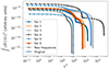 |
Fig. 3. L-curve for the best forward model (see Table 1) from each model set, with the regularisation parameter ranging from 103 to 1010. The x-axis is the goodness of fit, given by the χobs2. The y-axis shows the RLS penalty term, which is the integral of the square of the derivative of the profile. The optimal value for the regularisation according to the L-curve criterion should be in the hook of the L shapes in the profiles. |
The rotation profiles of the best fitting forward model (see Table 1) of each model set with their observational uncertainties are shown in Fig. 4. The full set of rotation profiles can be found in Appendix B. The different models show quite different behaviour in the rotation profiles, with most showing oscillating profiles, while only a few show a monotonic profile. This difference in behaviour is larger than the 2σ uncertainty regions, based on the observational uncertainties on the oscillation frequencies, including the lack of certainty regarding the identity of the symmetric component of the splittings. As these uncertainties include the range of splittings observed within one multiplet, they should not be considered to be statistical uncertainties but rather as giving a qualitative indication of frequency uncertainties. Overall, the difference between the models in the specific model sets and the observational uncertainties show smaller differences than between the different model sets. This indicates that the forward modelling, and specifically the mode identification, is the main source of uncertainty on the inverted profiles, making it challenging to draw conclusions about the rotation profiles. We can also see this in the rotation kernels (see Fig. 5), which change appreciably between different models. The rotation kernels define the relation between the observed frequencies and the rotation profile in the star. Therefore, if the rotation kernels change significantly, either because the mode identification is different or the internal structure of the model is changed, so too does the rotation profile.
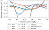 |
Fig. 4. Rotation profiles for the best model of each model set, with a regularisation parameter set to the maximum possible value such that the profiles still reproduce the observed splitting (see the main text for details). The bands around the profiles show the propagated 2σ uncertainties, including the lack of certainty regarding the identity of the symmetric component of the splittings. The dash-dotted red line shows the rotation profile obtained by Mombarg et al. (2023) using the ESTER code. The rotation profile of the best asteroseismic model of set 4 ranges from −1.2 d−1 to 0.7 d−1. |
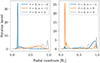 |
Fig. 5. Rotation kernels used in the rotation inversions for two of the forward models. Left panel: Best model of the original model set. Right panel: Best model for the new-frequencies model set. This plot shows how different the kernels of the different forward models can be. When matched to the same observations, the output from the rotation inversion can vary significantly from model to model. |
We find, from considering the rotation profiles for all the forward models, that the additional modes considered for model sets 1 through 6 do exclude a monotonic decreasing profile. This is not the case for the original and new-frequencies model sets, where some models can still be described adequately with monotonic decreasing profiles (see Figs. B.1 and B.2).
Figure 6 shows the centre to near-surface rotation ratios for all the models in our model sets. The rotation profiles were chosen in the same way as in the previous paragraph. We find that large ratios of the core and surface rotation rates (i.e. > 5) are not required by the observations, and that most profiles have a similar centre and near-surface rotation rate. This does not mean that the rotation profiles themselves are near rigid, as can be seen in Fig. 4. We note that the actual surface rotation rate for some of the models in model set 5 are close to zero, which would make the core-to-surface rotation rate ill-defined. Hence, we took the rotation rate at 0.8 R⋆ in the envelope as an approximation for the surface rotation rate.
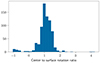 |
Fig. 6. Ratio of the rotation frequency in the centre of the star and at a radius of 0.8 R⋆. This choice of surface point was made to prevent ‘pathological’ values, as for some of the model sets the profiles tend to values around zero for the surface rotation rate. |
The projected surface rotational velocity was obtained from spectroscopic observations by Burssens et al. (2023) and found to be  km s−1. Given the possible range in stellar radii obtained from the forward modelling, the lower limit on the rotation frequency would be roughly 0.035 d−1, which is in line with the results we obtain here, as most of the surface rotation rates are in the range 0.1 d−1 to 0.3 d−1. Only some of the models in model set 5 would be inconsistent with this lower limit (see Fig. B.7).
We experimented with changing the parameters for the RLS: changing the number of spline knots to add and their position, and switching the first derivative regularisation to a second derivative regularisation. We find that the effects of changing the knots are negligible compared to the differences between the model structures. We tested whether placing knots non-uniformly to better match the sensitivity of the kernels mattered, but again found no significant changes. However, changing the regularisation function did affect the results, leading to rotation profiles with a much larger amplitude, although the locations of the peaks and valleys are similar to those of the profiles from the first derivative regularisation. Therefore, a regularisation based on the second derivative yields unphysical results.
Finally, we compared our rotation profiles to the rotation profile obtained by Mombarg et al. (2023) using the 2D code ESTER (see Fig. 4). As the model was calibrated to the rotation rate at the surface found by Burssens et al. (2023), we find that the value for the surface rotation rate matches with our results. The results from Mombarg et al. (2023) predict a monotonic increase from a rotation rate of 0.2 d−1 at the surface to 0.4 d−1 at the centre of the star and are in good agreement with some of the profiles in our solution sets. However, most of our 1D solutions are not monotonically increasing. While ESTER includes important elements of modelling the rotation profile in a star, such as meridional circulation, in a self-consistent way, there are still aspects in terms of angular momentum transport that are not included, such as internal gravity waves (e.g. Talon & Charbonnel 2005; Rogers 2015) or magnetic fields (Mestel & Weiss 1987; Spruit 2002; Fuller et al. 2019), which are relevant for stellar evolution (Aerts et al. 2019). Furthermore, 1D evolution codes such as MESA can include other important descriptions of physical processes, notably CBM and other forms of mixing, that ESTER models do not include in the implementation used by Mombarg et al. (2023). While these results are too uncertain at this point to speculate on which transport mechanism needs to be considered or tweaked, this discrepancy still indicates that modifications to ESTER and/or aspects of the asteroseismic modelling need to be made, as subjects of future work.
4. Rotational asymmetries of HD 192575
4.1. Higher-order effects of rotation
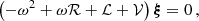
Rotation has at least two main effects on the pulsation frequencies of a star. It changes the evolution of a star through various transport processes and it causes a non-spherical deformation of the structure of the star, making it oblate (e.g. Maeder 2009). Secondly, the linearised pulsation equations gain linear and quadratic terms in the rotation frequency due to the Coriolis acceleration, the centrifugal acceleration, and the rotational shear. In combination with the structure changes from the star not being spherically symmetric, the solutions to the modified oscillation equations are no longer separable in r and θ. This means that one needs to either make simplifying approximations, as we do in this paper, or use 2D oscillationcomputations (Reese et al. 2006; Ouazzani et al. 2012). So far, modelling of asymmetric splittings in β Cep pulsators have been limited, with the studies by Pamyatnykh et al. (2004), Briquet et al. (2007), Suárez et al. (2009), and Guo et al. (2024) as notable exceptions. Here we go beyond their treatments in our modelling of HD 192575’s asymmetric low-order mode splittings, building upon the extensive modelling by Burssens et al. (2023) and the high-precision TESS-based observations.
Given the moderate rotation rate (∼16% of the Keplerian critical rotation rate) of HD 192575, we used a perturbative method to obtain the oscillation frequencies for a radially differential rotation profile, based on the formalisms of Saio (1981) and Lee & Baraffe (1995). The oscillation equations we considered here contain the Coriolis force term, the structure deformation of the stellar model due to the rotation, the coupling between spherical harmonics with different degrees, and both the poloidal and toroidal components of the vector spherical harmonics. The deformation of the stellar structure is computed using the Chandrasekhar-Milne expansion (Chandrasekhar 1933) up to the second order P2 contribution. This assumes a constant rotation rate, which is not what we find for this star. However, as the deformation is caused by the balance of the gravitational acceleration and the centrifugal acceleration, it is mostly felt in the outer layers of the star. We therefore approximated the deformation using the rotation rate near the surface. To compute other terms in the oscillation equation, we used the actual differential rotation profile, notably to evaluate the Coriolis force term.
We initially computed solutions of simplified oscillation equations consisting of the poloidal components of a single spherical harmonic. This simplified system consists of the non-rotating terms and the Coriolis acceleration. Since this is still a 1D system, these equations can be solved non-perturbatively. The solution for the poloidal component is valid up to first order in the rotation frequency. The Coriolis force also couples with the toroidal components of the ℓ ± 1 spherical harmonics. We computed these components using analytical expressions (e.g. Eqs. (32) and (33) of Saio 1981), which are also valid up to first order in the rotation frequency. The combined poloidal and toroidal components are similar to the zeroth order system considered by Soufi et al. (1998). This does not yet include the deformation of the stellar model by rotation and the feedback of the toroidal components of adjacent spherical degrees through the Coriolis force, both of which are second order in the rotation frequency.
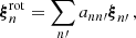
We then approximated the eigenfunction of each oscillation mode for the full oscillation equations as a linear combination of eigenfunctions initially obtained from the simplified oscillation equations:
 (2)
(2)
Due to the azimuthal symmetry of the rotation, this linear combination only consists of oscillation modes with the same azimuthal order. While in principle the sum over k′ is a sum over all radial orders and degrees, this is not possible in practice, and some truncation is needed. Substituting this linear expansion in the full oscillation equations yields a quadratic eigenvalue problem for coefficients akk′ and the oscillation frequency (ω) as the eigenvalue. More details on how such an eigenvalue problem can be solved can be found in Appendix C. The physical terms included in this perturbation are the stellar deformation up to the P2 Legendre polynomial, and the coupling with the toroidal modes through the Coriolis force. This method is fundamentally the same as the methods described by Saio (1981), Lee & Baraffe (1995), and Soufi et al. (1998), without the need to consider which modes should be included in computing near-degeneracy effects.
The perturbation method was validated with the 2D oscillation code TOP (Reese et al. 2006) and shown to be sufficiently accurate to model the measured mode asymmetries of HD 192575. Detailed comparisons of our method and 2D computations with ESTER/TOP will be described elsewhere (Mombarg et al., in prep.).
4.2. Observed asymmetries
We defined the asymmetries of a multiplet in the same way as Burssens et al. (2023), namely as the difference between two adjacent splittings, such that
 (3)
(3)
For the quadrupole multiplets we therefore have 𝒜0, 𝒜1, and 𝒜2, which do not need to have the same value.
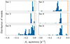 |
Fig. 7. Distribution of the theoretical asymmetries for the ℓ = 1 multiplet. Each panel is a different set, as indicated in the top-left corner of the panel. The vertical orange line indicates the observed asymmetry. The radial orders associated with these asymmetries can be found in Table 2 under the trip1 multiplet. |
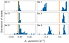 |
Fig. 8. Distribution of the theoretical 𝒜1 asymmetries for the quad1 ℓ = 2 multiplet. Each panel is a different set, as indicated in the top-left corner of the panel. The vertical orange line indicates the observed asymmetry. Since the multiplet is not complete, the 𝒜1 asymmetries have two observed values, which can be seen in the left panels as the two separate lines. The scale of the x-axis in the right panel is too large to show the two values. The radial orders associated with these asymmetries can be found in Table 2 under the quad1 multiplet. |
In the case of model sets 1 through 6, the single dipole mode multiplet always has a negative asymmetry (see Fig. 7). The bulk of the models show an asymmetry of the order of −0.1 d−1, which means that the distance between the retrograde mode and the zonal mode is about twice the distance between the zonal mode and the prograde mode. The exact value varies significantly (up to about −0.6 d−1), depending on the rotation frequency at the surface. The observed asymmetry on the other hand, is of the order of 0.001 d−1, more than two orders of magnitude smaller and positive. Some of the models do get close to the observed values. These correspond to models from model sets 3 and 5 with low surface rotation rates (see Figs. B.5 and B.7). Out of the 600 models in model sets 1 through 6, 16 are within a value of 0.01 d−1 from the observed value.
For the quadrupole modes, we find the asymmetries to be smaller by an order of magnitude for the same stellar models. This can be seen in Fig. 8, which shows the 𝒜1 asymmetry for the quad1 multiplet. Due to this multiplet only showing four of the five peaks needed for a full ℓ = 2 multiplet, the 𝒜1 asymmetry has two possible observed values associated with it. Only one of the values needs to fit the theoretical values, although both of them in the case of model sets 1, 3, and 5. While we only show model sets 1 through 6, the results are similar for the original and new-frequencies model sets. The original model set is able to fit the data similarly well as sets 1, 3, and 5, while the new-frequencies model set behaves similar to the other sets. Given the two options for the 𝒜1 asymmetry, we needed to fit either the 𝒜0 asymmetry or the 𝒜2 asymmetry. We find that this is indeed feasible, and therefore it is possible to reproduce the asymmetries for this multiplet. Of the remaining multiplets, we can reproduce the order of magnitude of the asymmetries of the quint1a multiplet with some of the model sets, as the theoretical g-mode asymmetries are smaller in this regime than the p-mode asymmetries. The trip2 multiplet is harder to reproduce, given its low asymmetry, with only set 3 being able to reproduce trip2. We provide supporting figures for all asymmetries not shown here in Appendix D.
The asymmetries are strongly dependent on the individual model and its rotation profile. Compared to the observational uncertainties, which are at least one order of magnitude smaller than the observed asymmetries, these asymmetries span a wide range of values. We indicate which rotation profiles have corresponding asymmetries that are within [0, 2𝒜] for all components of the observed quad1 and quint1a asymmetries in Figs. B.1 through B.8.
4.3. Discussion
Our results show a variation in the rotation profiles and, therefore, the corresponding theoretical asymmetries. While these rotation profiles all provide a reasonable match with the symmetric parts of the observed rotationally split multiples, this is not the case for the trip1 and trip2 multiplets, and for a subset of the models for the quint1a and quad2 multiplets. Hence, the observed asymmetries could be used to constrain both the rotation profile and the selection of the best forward model. In order to fully benefit from this information, the forward modelling procedure and subsequent fitting and computational steps should be combined into one overarching modelling procedure. It is encouraging, however, that our method finds asymmetries that are in agreement with the observations for two of the four multiplets, given that these were not considered at all during the stellar model selection process described in Sect. 2.
While improving the fitting procedures will lead to a more self-consistent analysis, there is still a discrepancy between the possible models and the observations for the trip1 and trip2 multiplets. Several potential explanations for this discrepancy between the theoretical and observed asymmetries exist. First and foremost, the 1D stellar models may not capture all the relevant physics needed to fully explain such detailed properties of the oscillation frequencies. Second, the impact of the chosen chemical mixture for the models may be sub-optimal choices, impacting the mode cavities and kernel computations. Third, a potential magnetic field, depending on its obliquity angle with the rotation axis, could counteract the rotational asymmetries (e.g. Loi 2021). One of the alternative explanations of the double quint1a and quint1b multiplets in HD 192575 is the presence of such an internal magnetic field. Finally, non-linear mode coupling may bring the asymmetries of the modes closer to zero (Buchler et al. 1995, 1997). Our results are therefore suitable to be used in the future, with the aim to measure and constrain these properties in more detail.
5. Conclusions
In this study we performed an updated asteroseismic modelling of the β Cep pulsator HD 192575, including new TESS mission data. We fitted rotation profiles and compared theoretical multiplet asymmetries with the observed asymmetries. Our asteroseismic modelling results are based on more, and more precise, observables than those used by Burssens et al. (2023). Keeping this in mind, our results agree well with the earlier ones from Burssens et al. (2023). Uncertainty in the mode identification of the observed pulsation multiplets leads to a larger uncertainty on the age, as well as on the mass and radius of the convective core, of HD 192575. While the initial mass, initial metallicity, and CBM have similar uncertainties due to degeneracies among these parameters, the uncertainty on the central hydrogen fraction has increased from 0.075 to about 0.3, and the uncertainty on the inferred mass and radius of the convective core has increased by a factor of 2.
For a selection of 742 forward models within the resultant 2σ confidence intervals of the best solution, we obtained rotation profiles using RLS inversions. The rotation profiles show a variety of behaviours: some have differential rotation of the order of only 20%, while some profiles yield counter-rotating regions. While this may seem like a wide variety of options, we stress that the rotation frequency within the star is below 0.4 d−1 for almost all profiles; this is in agreement with Burssens et al. (2023) and offers a remarkable calibration for theories of transport processes in massive stars. The main uncertainty on the rotation profiles originates from the large differences among the 742 models owing to the mode identification and theoretical uncertainties in (1D) stellar evolution theory. While drawing firm conclusions about the properties of the rotation profile is challenging given these theoretical uncertainties, almost all forward models favour weak differential rotation, and the resultant core-to-surface rotation ratio is at most a factor of 2 for almost all models.
We computed theoretical asymmetries from the rotation profiles and compared these asymmetries with the observed asymmetries. These computations include the effect of the Coriolis force and stellar deformation. For two of the four multiplets, we find agreement between our model grid and the observed asymmetries, while for the other two multiplets the theoretical asymmetries are larger than the observed asymmetries. We obtain different variations in computed asymmetries depending on the mode identification and individual stellar model.
Our results show that the rotation profile and the associated asymmetries provide a valuable tool for further constraining the evolutionary properties of HD 192575, and in particular the details of angular momentum transport in massive pulsating stars. To make maximal use of this information, we suggest that future endeavours to model this star combine the forward modelling, rotation inversion, and computations of the asymmetries in a self-consistent modelling framework. Such a framework currently does not exist but could pave the way towards modelling more aspects of the evolution of the star, such as its internal magnetic field properties.
Acknowledgments
The authors appreciated the critical comments from the referee, which encouraged V.V. to embark upon a new code development sprint. V.V. gratefully acknowledges support from the Research Foundation Flanders (FWO) under grant agreement N°1156923N (PhD Fellowship) and N°K233724N (Travel grant). D.M.B. gratefully acknowledges support from the Research Foundation Flanders (FWO; grant number: 1286521N), and UK Research and Innovation (UKRI) in the form of a Frontier Research grant under the UK government’s ERC Horizon Europe funding guarantee (SYMPHONY; grant number: EP/Y031059/1), and a Royal Society University Research Fellowship (URF; grant number: URF\R1\231631). S.B.D. acknowledges funding from the European Union’s Horizon 2020 research and innovation programme under the Marie Skłodowska-Curie grant agreement No 101034413. L.B. gratefully acknowledges support from the European Research Council (ERC) under the Horizon Europe programme (Calcifer; Starting Grant agreement N°101165631). S.M. acknowledges support from the PLATO CNES grant at CEA/DAp.C.A. acknowledges financial support from the Research Foundation Flanders (FWO) under grant K802922N (Sabbatical leave); she is grateful for the kind hospitality offered by CEA/Saclay during her sabbatical work visits in the spring of 2023. The research leading to these results has received funding from the European Research Council (ERC) under the Horizon Europe programme (Synergy Grant agreement N°101071505: 4D-STAR). While funded by the European Union, views and opinions expressed are however those of the author(s) only and do not necessarily reflect those of the European Union or the European Research Council. Neither the European Union nor the granting authority can be held responsible for them. The TESS data presented in this paper were obtained from the Mikulski Archive for Space Telescopes (MAST) at the Space Telescope Science Institute (STScI), which is operated by the Association of Universities for Research in Astronomy, Inc., under NASA contract NAS5-26555. Support to MAST for these data is provided by the NASA Office of Space Science via grant NAG5-7584 and by other grants and contracts. Funding for the TESS mission was provided by the NASA Explorer Program.
References
- Aerts, C., & De Cat, P. 2003, Space Sci. Rev., 105, 453 [CrossRef] [Google Scholar]
- Aerts, C., & Tkachenko, A. 2024, A&A, 692, R1 [NASA ADS] [CrossRef] [EDP Sciences] [Google Scholar]
- Aerts, C., Thoul, A., Daszyńska, J., et al. 2003, Science, 300, 1926 [Google Scholar]
- Aerts, C., Molenberghs, G., Michielsen, M., et al. 2018, ApJS, 237, 15 [Google Scholar]
- Aerts, C., Mathis, S., & Rogers, T. M. 2019, ARA&A, 57, 35 [Google Scholar]
- Belkacem, K., Marques, J. P., Goupil, M. J., et al. 2015, A&A, 579, A31 [NASA ADS] [CrossRef] [EDP Sciences] [Google Scholar]
- Bétrisey, J., Eggenberger, P., Buldgen, G., Benomar, O., & Bazot, M. 2023, A&A, 673, L11 [NASA ADS] [CrossRef] [EDP Sciences] [Google Scholar]
- Bharati Das, S., Einramhof, L., & Bugnet, L. 2024, A&A, 690, A217 [NASA ADS] [CrossRef] [EDP Sciences] [Google Scholar]
- Bhattacharya, S., Das, S. B., Bugnet, L., Panda, S., & Hanasoge, S. M. 2024, ApJ, 970, 42 [NASA ADS] [CrossRef] [Google Scholar]
- Bowman, D. M. 2020, Front. Astron. Space Sci., 7, 70 [Google Scholar]
- Bowman, D. M., & Michielsen, M. 2021, A&A, 656, A158 [NASA ADS] [CrossRef] [EDP Sciences] [Google Scholar]
- Briquet, M., Morel, T., Thoul, A., et al. 2007, MNRAS, 381, 1482 [Google Scholar]
- Buchler, J. R., Goupil, M. J., & Serre, T. 1995, A&A, 296, 405 [NASA ADS] [Google Scholar]
- Buchler, J. R., Goupil, M. J., & Hansen, C. J. 1997, A&A, 321, 159 [NASA ADS] [Google Scholar]
- Bugnet, L. 2022, A&A, 667, A68 [NASA ADS] [CrossRef] [EDP Sciences] [Google Scholar]
- Bugnet, L., Prat, V., Mathis, S., et al. 2021, A&A, 650, A53 [NASA ADS] [CrossRef] [EDP Sciences] [Google Scholar]
- Burssens, S., Bowman, D. M., Michielsen, M., et al. 2023, Nat. Astron., 7, 913 [NASA ADS] [CrossRef] [Google Scholar]
- Cantiello, M., Mankovich, C., Bildsten, L., Christensen-Dalsgaard, J., & Paxton, B. 2014, ApJ, 788, 93 [Google Scholar]
- Ceillier, T., Eggenberger, P., García, R. A., & Mathis, S. 2013, A&A, 555, A54 [NASA ADS] [CrossRef] [EDP Sciences] [Google Scholar]
- Chandrasekhar, S. 1933, MNRAS, 93, 390 [NASA ADS] [CrossRef] [Google Scholar]
- Christensen-Dalsgaard, J., Schou, J., & Thompson, M. J. 1990, MNRAS, 242, 353 [NASA ADS] [Google Scholar]
- Deheuvels, S., García, R. A., Chaplin, W. J., et al. 2012, ApJ, 756, 19 [Google Scholar]
- Deheuvels, S., Doğan, G., Goupil, M. J., et al. 2014, A&A, 564, A27 [NASA ADS] [CrossRef] [EDP Sciences] [Google Scholar]
- Deheuvels, S., Li, G., Ballot, J., & Lignières, F. 2023, A&A, 670, L16 [NASA ADS] [CrossRef] [EDP Sciences] [Google Scholar]
- Di Mauro, M. P., Ventura, R., Cardini, D., et al. 2016, ApJ, 817, 65 [NASA ADS] [CrossRef] [Google Scholar]
- Di Mauro, M. P., Ventura, R., Corsaro, E., & Moura, B. L. D. 2018, ApJ, 862, 9 [NASA ADS] [CrossRef] [Google Scholar]
- Dupret, M.-A., Thoul, A., Scuflaire, R., et al. 2004, A&A, 415, 251 [NASA ADS] [CrossRef] [EDP Sciences] [Google Scholar]
- Dziembowski, W. A., & Pamyatnykh, A. A. 2008, MNRAS, 385, 2061 [NASA ADS] [CrossRef] [Google Scholar]
- Eggenberger, P., Montalbán, J., & Miglio, A. 2012, A&A, 544, L4 [NASA ADS] [CrossRef] [EDP Sciences] [Google Scholar]
- Espinosa Lara, F., & Rieutord, M. 2013, A&A, 552, A35 [NASA ADS] [CrossRef] [EDP Sciences] [Google Scholar]
- Fritzewski, D. J., Vanrespaille, M., Aerts, C., et al. 2025, A&A, 698, A253 [NASA ADS] [CrossRef] [EDP Sciences] [Google Scholar]
- Fuller, J., Lecoanet, D., Cantiello, M., & Brown, B. 2014, ApJ, 796, 17 [Google Scholar]
- Fuller, J., Piro, A. L., & Jermyn, A. S. 2019, MNRAS, 485, 3661 [NASA ADS] [Google Scholar]
- Goldstein, J., & Townsend, R. H. D. 2020, ApJ, 899, 116 [NASA ADS] [CrossRef] [Google Scholar]
- Gough, D. O., & Thompson, M. J. 1990, MNRAS, 242, 25 [Google Scholar]
- Goupil, M. J., Mosser, B., Marques, J. P., et al. 2013, A&A, 549, A75 [NASA ADS] [CrossRef] [EDP Sciences] [Google Scholar]
- Guo, Z., Bedding, T. R., Pamyatnykh, A. A., et al. 2024, MNRAS, 535, 2927 [Google Scholar]
- Hansen, P. C. 2001, Computational Inverse Problems in Electrocardiology (WIT Press), 119 [Google Scholar]
- Hatta, Y., Sekii, T., Takata, M., & Kurtz, D. W. 2019, ApJ, 871, 135 [NASA ADS] [CrossRef] [Google Scholar]
- Hatta, Y., Sekii, T., Benomar, O., & Takata, M. 2022, ApJ, 927, 40 [NASA ADS] [CrossRef] [Google Scholar]
- Jermyn, A. S., Bauer, E. B., Schwab, J., et al. 2023, ApJS, 265, 15 [NASA ADS] [CrossRef] [Google Scholar]
- Kurtz, D. W., Saio, H., Takata, M., et al. 2014, MNRAS, 444, 102 [Google Scholar]
- Lee, U., & Baraffe, I. 1995, A&A, 301, 419 [NASA ADS] [Google Scholar]
- Li, G., Deheuvels, S., Ballot, J., & Lignières, F. 2022, Nature, 610, 43 [NASA ADS] [CrossRef] [Google Scholar]
- Loi, S. T. 2021, MNRAS, 504, 3711 [NASA ADS] [CrossRef] [Google Scholar]
- Maeder, A. 2009, Physics, Formation and Evolution of Rotating Stars, Astronomy and Astrophysics Library (Berlin, Heidelberg: Springer) [Google Scholar]
- Mahalanobis, P. C. 1936, Proc. Natl. Inst. Sci. India, 2, 49 [Google Scholar]
- Marques, J. P., Goupil, M. J., Lebreton, Y., et al. 2013, A&A, 549, A74 [NASA ADS] [CrossRef] [EDP Sciences] [Google Scholar]
- Mathis, S., & Bugnet, L. 2023, A&A, 676, L9 [NASA ADS] [CrossRef] [EDP Sciences] [Google Scholar]
- Mathis, S., & Zahn, J.-P. 2005, A&A, 440, 653 [NASA ADS] [CrossRef] [EDP Sciences] [Google Scholar]
- Mathis, S., Bugnet, L., Prat, V., et al. 2021, A&A, 647, A122 [EDP Sciences] [Google Scholar]
- Mestel, L., & Weiss, N. O. 1987, MNRAS, 226, 123 [Google Scholar]
- Mombarg, J. S. G., Rieutord, M., & Lara, F. E. 2023, A&A, 677, L5 [NASA ADS] [CrossRef] [EDP Sciences] [Google Scholar]
- Moyano, F. D., Eggenberger, P., Meynet, G., et al. 2022, A&A, 663, A180 [NASA ADS] [CrossRef] [EDP Sciences] [Google Scholar]
- Ouazzani, R.-M., Dupret, M.-A., & Reese, D. R. 2012, A&A, 547, A75 [NASA ADS] [CrossRef] [EDP Sciences] [Google Scholar]
- Ouazzani, R.-M., Marques, J. P., Goupil, M.-J., et al. 2019, A&A, 626, A121 [NASA ADS] [CrossRef] [EDP Sciences] [Google Scholar]
- Pamyatnykh, A. A., Handler, G., & Dziembowski, W. A. 2004, MNRAS, 350, 1022 [NASA ADS] [CrossRef] [Google Scholar]
- Paxton, B., Bildsten, L., Dotter, A., et al. 2011, ApJS, 192, 3 [Google Scholar]
- Paxton, B., Cantiello, M., Arras, P., et al. 2013, ApJS, 208, 4 [Google Scholar]
- Paxton, B., Marchant, P., Schwab, J., et al. 2015, ApJS, 220, 15 [Google Scholar]
- Paxton, B., Schwab, J., Bauer, E. B., et al. 2018, ApJS, 234, 34 [NASA ADS] [CrossRef] [Google Scholar]
- Paxton, B., Smolec, R., Schwab, J., et al. 2019, ApJS, 243, 10 [Google Scholar]
- Pijpers, F. P., & Thompson, M. J. 1994, A&A, 281, 231 [NASA ADS] [Google Scholar]
- Reese, D., Lignières, F., & Rieutord, M. 2006, A&A, 455, 621 [NASA ADS] [CrossRef] [EDP Sciences] [Google Scholar]
- Ricker, G. R., Winn, J. N., Vanderspek, R., et al. 2014, JATIS, 1, 014003 [NASA ADS] [Google Scholar]
- Rogers, T. M. 2015, ApJ, 815, L30 [Google Scholar]
- Rogers, T. M., Lin, D. N. C., McElwaine, J. N., & Lau, H. H. B. 2013, ApJ, 772, 21 [NASA ADS] [CrossRef] [Google Scholar]
- Saio, H. 1981, ApJ, 244, 299 [NASA ADS] [CrossRef] [Google Scholar]
- Salmon, S. J. A. J., Moyano, F. D., Eggenberger, P., Haemmerlé, L., & Buldgen, G. 2022, A&A, 664, L1 [NASA ADS] [CrossRef] [EDP Sciences] [Google Scholar]
- Schatzman, E. 1993, A&A, 279, 431 [NASA ADS] [Google Scholar]
- Soufi, F., Goupil, M. J., & Dziembowski, W. A. 1998, A&A, 334, 911 [NASA ADS] [Google Scholar]
- Spruit, H. C. 2002, A&A, 381, 923 [CrossRef] [EDP Sciences] [Google Scholar]
- Stankov, A., & Handler, G. 2005, ApJS, 158, 193 [NASA ADS] [CrossRef] [Google Scholar]
- Sterken, C., & Jerzykiewicz, M. 1993, Space Sci. Rev., 62, 95 [NASA ADS] [CrossRef] [Google Scholar]
- Suárez, J. C., Goupil, M. J., & Morel, P. 2006, A&A, 449, 673 [NASA ADS] [CrossRef] [EDP Sciences] [Google Scholar]
- Suárez, J. C., Moya, A., Amado, P. J., et al. 2009, ApJ, 690, 1401 [CrossRef] [Google Scholar]
- Takahashi, K., & Langer, N. 2021, A&A, 646, A19 [NASA ADS] [CrossRef] [EDP Sciences] [Google Scholar]
- Talon, S., & Charbonnel, C. 2005, A&A, 440, 981 [NASA ADS] [CrossRef] [EDP Sciences] [Google Scholar]
- Talon, S., Kumar, P., & Zahn, J.-P. 2002, ApJ, 574, L175 [Google Scholar]
- Townsend, R. H. D., & Teitler, S. A. 2013, MNRAS, 435, 3406 [Google Scholar]
- Townsend, R. H. D., Goldstein, J., & Zweibel, E. 2018, MNRAS, 475, 879 [NASA ADS] [CrossRef] [Google Scholar]
- Triana, S. A., Moravveji, E., Pápics, P. I., et al. 2015, ApJ, 810, 16 [Google Scholar]
- Triana, S. A., Corsaro, E., Ridder, J. D., et al. 2017, A&A, 602, A62 [NASA ADS] [CrossRef] [EDP Sciences] [Google Scholar]
- Zahn, J. P., Talon, S., & Matias, J. 1997, A&A, 322, 320 [NASA ADS] [Google Scholar]
Appendix A: New mode frequencies
The frequencies of the modelled multiplets derived from the combined cycle 2 and cycles 4 and 5 TESS observations can be found in Table A.1. We used the same names as Burssens et al. (2023) for these multiplets. While more frequencies can be found in this region, for example at 3.45 d−1 and 4.03 d−1, which do not fit in the existing pattern and hint at a third multiplet, we consider interpreting these frequencies beyond the scope of this work, which focuses on the rotation inversion.
Frequencies and spacings of the detected multiplets using the cycle 2 and cycles 4 and 5 TESS data.
Appendix B: Rotation profiles
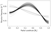 |
Fig. B.1. Rotation profiles obtained from the inversion method described in Sect. 3 for the original model set. The profiles shown have the lowest level of differential rotation while still fitting the observed splittings. |
The rotation profiles for all of the models obtained from the forward models can be found in Figures B.2 to B.8.
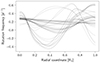 |
Fig. B.2. Same as Fig. B.1 but for the new-frequencies model set. |
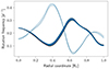 |
Fig. B.3. Same as Fig. B.1 but for model set 1. The blue profiles have asymmetries for the quad1 multiplet that are similar to the observed asymmetries (see Sect. 4.2 for details). |
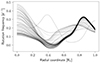 |
Fig. B.4. Same as Fig. B.1 but for model set 2. |
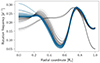 |
Fig. B.5. Same as Fig. B.1 but for model set 3. The blue profiles have asymmetries for the quad1 multiplet that are similar to the observed asymmetries (see Sect. 4.2 for details). |
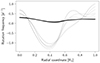 |
Fig. B.6. Same as Fig. B.1 but for model set 4. |
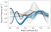 |
Fig. B.7. Same as Fig. B.1 but for model set 5. The blue and orange profiles have asymmetries for the quad1 and quint1a multiplet, respectively, that are similar to the observed asymmetries (see Sect. 4.2 for details). |
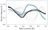 |
Fig. B.8. Same as Fig. B.1 but for model set 6. The blue profiles have asymmetries for the quad1 multiplet that are similar to the observed asymmetries (see Sect. 4.2 for details). |
Appendix c: Solving the quadratic eigenvalue problem
The main oscillation equation relevant for this paper is obtained by perturbing the equation of motion in the presence of a velocity field due to the rotation:
 (C.1)
(C.1)
For ease of notation, we write this equation as
 (C.2)
(C.2)
where the operator ℛ contains the terms linear in Ω, 𝒱 the terms quadratic in Ω, and ℒ the terms in the oscillation equation in absence of rotation. Given the assumption that the solutions to the rotating case are given by the linear combination
 (C.3)
(C.3)
we get the following set of equations by multiplying Eq. (C.2) by ξn from the left,
 (C.4)
(C.4)
for each n. The matrices Dnn′, Rnn′, Lnn′, and Vnn′ are given by the inner products < ξn, Xξn′> with X = 𝟙, ℛ, ℒ, and 𝒱, respectively. In the case of a vacuum outer boundary condition, the matrix D will be the identity matrix barring numerical errors, but this is not the case for more realistic boundary conditions. This can then be expressed as the generalised eigenvalue problem:
 (C.5)
(C.5)
Since this eigenvalue problem is quadratic in the eigenvalue (the frequency ω), we first converted this problem to a normal eigenvalue problem. Consider that a1 is a solution to the above equation with eigenvalue ω. We define a2 = ωa1 as a new vector, which leads us to the equation
 (C.6)
(C.6)
We combine these definition and equation as
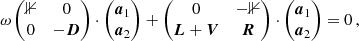 (C.7)
(C.7)
which is a linear generalised eigenvalue problem, and can be solved with standard methods.
Appendix D: All remaining asymmetry plots
Figures D.1 to D.8 show the asymmetries for model sets 1 through 6, for the multiplets and components of the multiplets that were not shown in the main text.
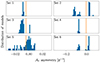 |
Fig. D.1. Distribution of the theoretical 𝒜0 asymmetries for the quad1 ℓ = 2 multiplet. Each panel is a different set, indicated in the top-left corner of the panel. The vertical orange line indicates the observed asymmetry. Since the multiplet is not complete, only one of the asymmetries, 𝒜0 or 𝒜2, must fit the data. The radial orders associated with these asymmetries can be found in Table 2 under the quad1 multiplet. |
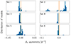 |
Fig. D.3. Distribution of the theoretical 𝒜0 asymmetries for the quint1a ℓ = 2 multiplet. Each panel is a different set, as indicated in the top-left corners. The vertical orange line indicates the observed asymmetry. The radial orders associated with these asymmetries can be found in Table 2 under the quinta multiplet. |
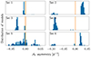 |
Fig. D.6. Distribution of the theoretical 𝒜0 asymmetries for the trip2 ℓ = 2 multiplet. Each panel is a different set, indicated in the top-left corner of the panel. The vertical orange line indicates the observed asymmetry. Since the multiplet is not complete, only one of the asymmetries, 𝒜0, 𝒜1, or 𝒜2, must fit the data. The radial orders associated with these asymmetries can be found in Table 2 under the trip2 multiplet. |
All Tables
Best model parameters and 2σ confidence intervals for the forward asteroseismic modelling of HD 192575 for the original modelling by Burssens et al. (2023) and our seven new modelling sets.
Mode identification of the multiplets used for the different model sets, given as (ℓ,npg).
Frequencies and spacings of the detected multiplets using the cycle 2 and cycles 4 and 5 TESS data.
All Figures
|
Fig. 1. Frequency spectrum of HD 192575. Top panel: Full frequency spectrum, with the regions with fitted modes indicated by the light blue boxes. Bottom panels: Zoomed-in views of those boxes. From left to right, the multiplets are given the names quint1a (blue, first panel), quint1b (orange, first panel), quad1 (blue, second panel), trip1 (blue, third panel), and trip2 (orange, third panel). |
| In the text | |
|
Fig. 2. Probability density function of observing one of the models at a certain central hydrogen fraction. The intervals (black) show the uncertainty regions for the central hydrogen fraction for each of the model sets (see Table 1). From top to bottom, the intervals show the original, new-frequencies, and sets 1 through 6 solutions. |
| In the text | |
|
Fig. 3. L-curve for the best forward model (see Table 1) from each model set, with the regularisation parameter ranging from 103 to 1010. The x-axis is the goodness of fit, given by the χobs2. The y-axis shows the RLS penalty term, which is the integral of the square of the derivative of the profile. The optimal value for the regularisation according to the L-curve criterion should be in the hook of the L shapes in the profiles. |
| In the text | |
|
Fig. 4. Rotation profiles for the best model of each model set, with a regularisation parameter set to the maximum possible value such that the profiles still reproduce the observed splitting (see the main text for details). The bands around the profiles show the propagated 2σ uncertainties, including the lack of certainty regarding the identity of the symmetric component of the splittings. The dash-dotted red line shows the rotation profile obtained by Mombarg et al. (2023) using the ESTER code. The rotation profile of the best asteroseismic model of set 4 ranges from −1.2 d−1 to 0.7 d−1. |
| In the text | |
|
Fig. 5. Rotation kernels used in the rotation inversions for two of the forward models. Left panel: Best model of the original model set. Right panel: Best model for the new-frequencies model set. This plot shows how different the kernels of the different forward models can be. When matched to the same observations, the output from the rotation inversion can vary significantly from model to model. |
| In the text | |
|
Fig. 6. Ratio of the rotation frequency in the centre of the star and at a radius of 0.8 R⋆. This choice of surface point was made to prevent ‘pathological’ values, as for some of the model sets the profiles tend to values around zero for the surface rotation rate. |
| In the text | |
|
Fig. 7. Distribution of the theoretical asymmetries for the ℓ = 1 multiplet. Each panel is a different set, as indicated in the top-left corner of the panel. The vertical orange line indicates the observed asymmetry. The radial orders associated with these asymmetries can be found in Table 2 under the trip1 multiplet. |
| In the text | |
|
Fig. 8. Distribution of the theoretical 𝒜1 asymmetries for the quad1 ℓ = 2 multiplet. Each panel is a different set, as indicated in the top-left corner of the panel. The vertical orange line indicates the observed asymmetry. Since the multiplet is not complete, the 𝒜1 asymmetries have two observed values, which can be seen in the left panels as the two separate lines. The scale of the x-axis in the right panel is too large to show the two values. The radial orders associated with these asymmetries can be found in Table 2 under the quad1 multiplet. |
| In the text | |
|
Fig. B.1. Rotation profiles obtained from the inversion method described in Sect. 3 for the original model set. The profiles shown have the lowest level of differential rotation while still fitting the observed splittings. |
| In the text | |
|
Fig. B.2. Same as Fig. B.1 but for the new-frequencies model set. |
| In the text | |
|
Fig. B.3. Same as Fig. B.1 but for model set 1. The blue profiles have asymmetries for the quad1 multiplet that are similar to the observed asymmetries (see Sect. 4.2 for details). |
| In the text | |
|
Fig. B.4. Same as Fig. B.1 but for model set 2. |
| In the text | |
|
Fig. B.5. Same as Fig. B.1 but for model set 3. The blue profiles have asymmetries for the quad1 multiplet that are similar to the observed asymmetries (see Sect. 4.2 for details). |
| In the text | |
|
Fig. B.6. Same as Fig. B.1 but for model set 4. |
| In the text | |
|
Fig. B.7. Same as Fig. B.1 but for model set 5. The blue and orange profiles have asymmetries for the quad1 and quint1a multiplet, respectively, that are similar to the observed asymmetries (see Sect. 4.2 for details). |
| In the text | |
|
Fig. B.8. Same as Fig. B.1 but for model set 6. The blue profiles have asymmetries for the quad1 multiplet that are similar to the observed asymmetries (see Sect. 4.2 for details). |
| In the text | |
|
Fig. D.1. Distribution of the theoretical 𝒜0 asymmetries for the quad1 ℓ = 2 multiplet. Each panel is a different set, indicated in the top-left corner of the panel. The vertical orange line indicates the observed asymmetry. Since the multiplet is not complete, only one of the asymmetries, 𝒜0 or 𝒜2, must fit the data. The radial orders associated with these asymmetries can be found in Table 2 under the quad1 multiplet. |
| In the text | |
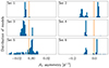 |
Fig. D.2. Same as Fig. D.1 but for the 𝒜2 asymmetry. |
| In the text | |
|
Fig. D.3. Distribution of the theoretical 𝒜0 asymmetries for the quint1a ℓ = 2 multiplet. Each panel is a different set, as indicated in the top-left corners. The vertical orange line indicates the observed asymmetry. The radial orders associated with these asymmetries can be found in Table 2 under the quinta multiplet. |
| In the text | |
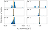 |
Fig. D.4. Same as Fig. D.3 but for the 𝒜1 asymmetry. |
| In the text | |
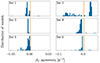 |
Fig. D.5. Same as Fig. D.3 but for the 𝒜2 asymmetry. |
| In the text | |
|
Fig. D.6. Distribution of the theoretical 𝒜0 asymmetries for the trip2 ℓ = 2 multiplet. Each panel is a different set, indicated in the top-left corner of the panel. The vertical orange line indicates the observed asymmetry. Since the multiplet is not complete, only one of the asymmetries, 𝒜0, 𝒜1, or 𝒜2, must fit the data. The radial orders associated with these asymmetries can be found in Table 2 under the trip2 multiplet. |
| In the text | |
 |
Fig. D.7. Same as Fig. D.6 but for the 𝒜1 asymmetry. |
| In the text | |
 |
Fig. D.8. Same as Fig. D.6 but for the 𝒜2 asymmetry. |
| In the text | |
Current usage metrics show cumulative count of Article Views (full-text article views including HTML views, PDF and ePub downloads, according to the available data) and Abstracts Views on Vision4Press platform.
Data correspond to usage on the plateform after 2015. The current usage metrics is available 48-96 hours after online publication and is updated daily on week days.
Initial download of the metrics may take a while.