| Issue |
A&A
Volume 701, September 2025
|
|
|---|---|---|
| Article Number | A179 | |
| Number of page(s) | 10 | |
| Section | Extragalactic astronomy | |
| DOI | https://doi.org/10.1051/0004-6361/202453082 | |
| Published online | 12 September 2025 | |
Identifying radio active galactic nuclei with machine learning and large-area surveys
1
School of Mathematics, Physics and Statistics, Shanghai University of Engineering Science, Shanghai 201620, People’s Republic of China
2
Center of Application and Research of Computational Physics, Shanghai University of Engineering Science, Shanghai 201620, People’s Republic of China
⋆ Corresponding author: This email address is being protected from spambots. You need JavaScript enabled to view it.
Received:
20
November
2024
Accepted:
30
July
2025
Abstract
Context. Active galactic nuclei (AGNs) and star-forming galaxies (SFGs) are the primary sources in the extragalactic radio sky. But it is difficult to distinguish the radio emission produced by AGNs from that by SFGs, especially when the radio sources are faint. Best et al. (2023, MNRAS, 523, 1729) classified the radio sources in LoTSS Deep Fields DR1 through multiwavelength SED fitting. With the classification results of them, we performed a supervised machine learning to distinguish radio AGNs and radio SFGs.
Aims. We aim to provide a supervised classifier to identify radio AGNs, which can get both high purity and completeness simultaneously, and can easily be applied to datasets of large-area surveys.
Methods. The classifications of Best et al. (2023, MNRAS, 523, 1729) were used as the true labels for supervised machine learning. With the cross-matched sample of LoTSS Deep Fields DR1, AllWISE, and Gaia DR3, the features of optical and mid-infrared magnitude and colors were applied to train the classifier. The performance of the classifier was evaluated mainly by the precision, recall, and F1 score of both AGNs and non-AGNs.
Results. By comparing the performance of six learning algorithms, CatBoost was chosen to construct the best classifier. The best classifier gets precision = 0.974, recall = 0.865, and F1 = 0.916 for AGNs, and precision = 0.936, recall = 0.988, and F1 = 0.961 for non-AGNs. After applying our classifier to the cross-matched sample of LoTSS DR2, AllWISE, and Gaia DR3, we obtained a sample of 49716 AGNs and 102261 non-AGNs. The reliability of these classification results was confirmed by comparing them with the spectroscopic classification of SDSS. The precision and recall of AGN sample can be as high as 94.2% and 92.3%, respectively. We also trained a model to identify radio excess sources. The F1 scores are 0.610 and 0.965 for sources with and without radio excess, respectively.
Key words: galaxies: active / galaxies: star formation / radio continuum: galaxies
© The Authors 2025
 Open Access article, published by EDP Sciences, under the terms of the Creative Commons Attribution License (https://creativecommons.org/licenses/by/4.0), which permits unrestricted use, distribution, and reproduction in any medium, provided the original work is properly cited.
This article is published in open access under the Subscribe to Open model. This email address is being protected from spambots. You need JavaScript enabled to view it. to support open access publication.
1. Introduction
Active galactic nuclei (AGNs) and star-forming galaxies (SFGs) are the most primary populations of extragalactic radio sky (Padovani 2016). Both of them are important for understanding the evolution of galaxies and supermassive black holes across cosmic time (Magliocchetti 2022). Relativistic jets in AGNs are believed to be the most powerful extragalactic radio sources. Traditionally, these type of AGNs hosting powerful jets are classified as radio-loud (RL) AGNs, which are defined through the ratio of radio to optical emission (Kellermann et al. 1989). In the faint radio sky, SFGs become numerically dominant over RL and radio-quiet (RQ) AGNs (Padovani 2016; Best et al. 2023).
Radio morphology is the direct method of identifying AGN jets. Powerful radio lobes and jets can be observed in bright radio AGNs at a resolution of arcseconds (Blandford et al. 2019). Detections of radio cores or low-power jets, which might be ubiquitous in RQ AGNs (Ho 2008), usually require the usage of high-sensitivity very long baseline interference observations at milliarcsecond resolution (Ulvestad et al. 2005; Wang et al. 2023). In addition to radio morphology, other radio properties, such as radio spectra and brightness temperature, are helpful to distinguish radio emission from AGNs and SFGs (Panessa et al. 2019; Morabito et al. 2022). To estimate these properties accurately, resolving radio cores and other radio structures is also preferred. Due to the limited angular resolution, the majority of extragalactic radio sources are still unresolved1 in current large-area radio surveys (Shimwell et al. 2022). Thus, it is difficult to identify jetted AGNs in large datasets by the information from radio observations alone (Magliocchetti 2022). Radio excess is then employed to identify jetted AGNs. In the literature, radio excess sources can be identified based on the deviation from the radio/far-infrared (FIR) correlation (Bonzini et al. 2015), from the radio/mid-infrared (MIR) correlation (Yao et al. 2022; Fan 2024), or from the radio–star formation rate (SFR) correlation (Best et al. 2023).
Apart from radio excess, other multiwavelength features are available to separate RQ AGNs and SFGs. Optical spectroscopy and multiwavelength spectral energy distribution (SED) fitting are two widely used methods. Quasars, galaxies, or stars can be classified by template matching in spectroscopic surveys, such as SDSS (Bolton et al. 2012; Lyke et al. 2020). Active galactic nuclei in galaxies can then be classified by the so-called BPT diagram (Baldwin et al. 1981). Other useful spectroscopic features to identify radio AGNs include Hα luminosity and 4000 Å break strength, which depend on the SFR and specific SFR, respectively (Best & Heckman 2012). Galaxy SED fitting is a technique to fit the multiwavelength photometric data with physical models involving stellar populations and dust radiation, which can derive the properties of the host galaxies. For several fitting codes, the radiation from AGNs are also considered. Thus the fraction of AGN contribution to observed SEDs can be determined (see Pacifici et al. 2023; Best et al. 2023 and references therein). In addition, infrared colors, optical colors, and X-ray properties are also used to select AGN candidates (Padovani 2016; Magliocchetti 2022).
As a high-z and high-luminosity subsample of AGNs, quasars are expected to have zero parallaxes and proper motions. Astrometric measurement is thus useful to distinguish quasars from stars (Shu et al. 2019; Gaia Collaboration 2023a). The largest advantage of astrometry-based AGN classification is that it is unbiased for selecting obscured AGNs. Obscured AGNs, whose radiation from accretion disk is obscured by dust, would be missed in optical color selected AGN samples. To avoid the contamination from distant stars, the AGN candidates classified based on astrometric information still need confirmation by their radiation properties (Heintz et al. 2018).
In recent years, the machine learning technique has been applied to astronomical data more frequently (Ball & Brunner 2010; Ivezić et al. 2014; Feigelson et al. 2021; Fotopoulou 2024), such as classifications of astronomical objects (Richards et al. 2011; Lochner et al. 2016; Busca & Balland 2018; Kang et al. 2019; Lao et al. 2023), the estimation of physical parameters (Carliles et al. 2010; Glauch et al. 2022; Lin et al. 2023; Zeraatgari et al. 2024), and analyses of astronomical images (Kuntzer et al. 2016; Ma et al. 2019; Boucaud et al. 2020; Dai et al. 2023). Although there are many works focusing on AGN and quasar classifications, which can identify the features of AGNs from photometric (Clarke et al. 2020; Fu et al. 2024), spectroscopic (Busca & Balland 2018; Tardugno Poleo et al. 2023), image (Ma et al. 2019; Guo et al. 2022), or time series data (Faisst et al. 2019; McLaughlin et al. 2024), few machine-learning-based classifications are performed to distinguish radio AGNs from radio SFGs.
Karsten et al. (2023) performed a supervised classification for radio AGNs and radio SFGs based on the multiwavelength data from Kondapally et al. (2021), including deep surveys of radio, infrared, optical, and ultraviolet bands. The classification labels used for their training were taken from Best et al. (2023), which were obtained from SED fitting. For AGNs, their classifier got a precision of 0.87 and a recall of 0.78. They also attempted to train their classifier with different combinations of photometric bands. For the training with fewer bands, the performance for AGNs became worse. The precision and recall especially did not reach their highest values with the same training features. A high precision was derived when all the features including redshift were considered, while high recall was favored when redshift was excluded (their Table 5). Another limitation of their classifier is that the training sample focused on several small sky areas where the coverage of multiwavelength data is plentiful. Their training features from radio to ultraviolet bands are hard to collect for larger sky areas currently. Thus it is difficult for their classifier to predict classifications using new datasets of large-area surveys.
In this paper, we create a supervised machine-learning-based classifier to identify radio AGNs, with true labels from the results of the Low Frequency Array (LOFAR) Two-metre Sky Survey (LoTSS) Deep Fields first data release (DR1) (Tasse et al. 2021; Sabater et al. 2021; Best et al. 2023), and training features from large-area surveys, i.e., AllWISE (Cutri et al. 2021) and Gaia DR3 (Gaia Collaboration 2023b). Then we apply it to the cross-matched catalog of LoTSS DR2 (Shimwell et al. 2022), AllWISE, and Gaia DR3. The reliability of the classifier is independently examined by comparing with the spectroscopic classifications of the Sloan Digital Sky Survey (SDSS) DR17 (Abdurro’uf et al. 2022). Section 2 describes the datasets we use, as well the evaluation metrics for machine leaning. In Sect. 3 we present our classifier with best performance. The classification results applied to unclassified large-area surveys are also given. In Sect. 4 the dependence on different groups of features, the reliability of our classifier, and the performance in identifying radio excess sources are discussed. Section 5 summarizes our main conclusions.
2. Dataset and method
Best et al. (2023) collected deep multiwavelength data and applied SED fitting for 81951 radio sources of LoTSS Deep Fields DR1. LoTSS Deep Fields is a deep sky survey with 6″ resolution and a targeted noise level of 10 − 15 μJy beam−1 at about 150 MHz. It covers about 25 deg2 of the northern sky in its first data release, which contains three fields (ELAIS-N1, Boötes, and Lockman Hole) (Tasse et al. 2021; Sabater et al. 2021). For these fields, deep multiwavelength data from ultraviolet to FIR are plentiful (Kondapally et al. 2021). Using the multiwavelength photometric data, Best et al. (2023) applied four different codes (named MAGPHYS, BAGPIPGS, CIGALE, and AGNFITTER) to fit the SEDs of radio sources in LoTSS Deep Fields DR1. Two SED fitting codes, MAGPHYS and BAGPIPGS, only account for the emission from stars and dust inside the galaxies. Thus, they would show poor reliability when they were applied to fit AGNs. The other two, CIGALE and AGNFITTER, consider the extra emission from AGNs, and can determine the AGN fraction based on the contribution from torus. Combining the estimations of the AGN fraction and fitting reliability of the four codes, they separated the sources with and without AGN contributions to their SEDs, i.e., AGNs and non-AGNs.
The SFR can also be estimated by all the four SED fitting codes. In Best et al. (2023), they used the consensus value of the SFR to maximize the advantage of different codes. For AGNs, the SFR estimations by CIGALE were favored. The SFR estimations by AGNFITTER were used only when the fittings of CIGALE were considered to be unreliable. For non-AGNs, the mean SFRs of MAGPHYS and BAGPIPGS were used. Based on the consensus SFRs, Best et al. (2023) derived a relation between the radio luminosity and the SFRs, whereby the radio luminosities are expected from the SF activities. Then they identified radio excess sources through the offset to a large radio luminosity relative to this radio-SFR relation. Combining the classification of AGNs and radio excess sources, Best et al. (2023) classified radio sources into SFGs, RQ AGNs, low-excitation radio galaxies (LERGs), and high-excitation radio galaxies (HERGs) in LoTSS Deep Fields DR1. Sources with neither AGN contributions to their SEDs nor radio excess are classified as SFGs. Sources with AGN contributions but no radio excess are classified as RQ AGNs. Sources with radio excess can be divided into LERGs and HERGs based on the absence or presence of AGN SEDs, respectively. In this paper, we use the binary classifications of AGNs and non-AGNs2 in Best et al. (2023) as the labels to train the data.
To identify new radio AGNs with large datasets, we prefer to select the multiwavelength photometric data of large-area surveys as the features for training. Although ultraviolet, X-ray, and γ-ray observations are useful for AGN selection, the sensitivities and sample sizes of current surveys at these bands are still limited compared with those at low energy bands. Thus we only considered radio, infrared, and optical surveys to construct our samples for machine learning.
The Wide-field Infrared Survey Explorer (WISE) surveys the MIR sky at 3.4, 4.6, 12, and 22 μm (W1, W2, W3, and W4, respectively) (Wright et al. 2010). It has been suggested that AGNs are located at an unique region on the WISE color-color diagram due to the external contributions from torus, which prompts several AGN selection criteria based on WISE MIR colors (Jarrett et al. 2011; Stern et al. 2012; Mateos et al. 2012; Assef et al. 2013). Optical colors are also widely used to selected AGN/quasar candidates, which are bluer for AGNs than those for stars and normal galaxies due to radiation from the accretion disks of AGNs (Peterson 1997; Euclid Collaboration: Bisigello et al. 2024). SDSS is one of most famous optical surveys with both multiband imaging and spectroscopy. Its photometry is performed with five filters, u, g, r, i, and z (York et al. 2000). The Gaia space mission aims to measure the three-dimensional spatial distribution of billions of astronomical objects with high-accuracy astrometry and spectrophotometry (Gaia Collaboration 2016). Its third data release provides precise celestial positions, proper motions, parallaxes, and three-broadband photometry in G, BP, and RP for more than a billion sources across the entire sky (Gaia Collaboration 2023b).
To construct the sample for machine learning and collect multiband photometric data points as training features, we cross-matched LoTSS Deep Fields DR1 with AllWISE and Gaia DR3 with TOPCAT (Taylor 2005). The radii in the cross-matching were all set to 1″ to avoid spurious matches through this paper. After the cross-matching, we excluded the sources with no magnitude measurements of the W1, W2, W3, W4, G, BP, and RP bands3, as well as those with null values of magnitude errors in AllWISE. The later is for the 2σ detection of AllWISE4. This resulted in a sample with 1698 sources, which contains 594 AGNs, 1101 non-AGNs, 160 sources with radio excess, and 1491 sources without radio excess. This sample (hereafter the main sample) was used for the supervised machine learning, which includes the classification labels from Best et al. (2023), integrated radio flux density from LoTSS Deep Fields DR1, MIR photometric magnitudes of W1, W2, W3, and W4 from AllWISE, and magnitudes of G, BP, RP, and two astrometric parameters (proper motion and parallax) from Gaia DR3. Two astrometric features are only used when their importance is evaluated in Sect. 4.1.
The main sample with features and labels was then split into two parts. Seventy percent of sources were used as a training set, while the remaining thirty percent were taken as a test set. The classifier was trained on the training set, while the test set was used to evaluate the performance of the classifier. The performance of the classifier with machine learning can be evaluated by several metrics, such as accuracy, precision, recall, and F1 score. The accuracy score returns the fraction for which the predicted labels match the true labels. It is a simple indicator to evaluate the overall results of machine learning. Its value is dominated by the majority class when the numbers of the both classes are imbalanced. Precision presents the ability of the classifier to predict true labels of each class, and recall presents the ability of the classifier to find all the true labels of each class. Precision and recall correspond to the purity and completeness of a sample, respectively. The F1 score is the harmonic mean of precision and recall, whereby the relative contributions of precision and recall are equal. The definition of the above metric is as follows:
 (1a)
(1a)
 (1b)
(1b)
 (1c)
(1c)
 (1d)
(1d)
where I(x) is the indicator function. When ytrue, i = yprediction, i it returns 1; otherwise, it returns 0. The TP, TN, FP, and FN refer to the number of true positives, true negatives, false positives, and false negatives, respectively.
In general, if two types of sources have overlapping parameter spaces, a classification criterion has difficulty achieving high purity and completeness simultaneously. Improving purity often means excluding more potential candidates, which reduces the completeness. On the contrary, improving completeness would result in candidates with low reliability being included. The machine learning technique may improve the situation with multidimensional features. In order to evaluate how the classifier addresses this issue, both precision and recall are presented in this paper. As a metric considering both precision and recall, the F1 score is the ideal indicator to evaluate the overall performance of a classifier. It was thus used to derive the optimal algorithms and hyperparameters. In addition, the sample of AGNs and non-AGNs in the main sample are imbalanced; thus, the metrics of both classes were taken into account individually, especially the minority sample, AGNs. Accuracy was only used to evaluate feature importance (see Sect. 4.1). The confusion matrix, whereby the numbers of true and false predictions for each class are visually presented, was also used to check the performance of our classifier. In the best-case scenario, the confusion matrix is expected to be purely diagonal, with nonzero elements on the diagonal, and zero elements otherwise (Baron 2019).
The receiver operating characteristic (ROC) curve, as well as the area under the curve (AUC) were applied to visually compare different algorithms of machine learning (Bradley 1997; Baron 2019). The Y axis and X axis of the ROC curve show the true positive rate (TPR) and the false positive rate (FPR), which correspond to recall of AGNs and 1 − recall of non-AGNs, respectively. A perfect machine learning model will get recall = 1 for both classes. That means AUC also equals 1.
3. Results of machine learning
3.1. The classifier with the best performance
The performance of a machine learning model can be affected by several factors, such as the datasets, the features of training, the learning algorithms, and the hyperparameters of the learning algorithms. We firstly compare the performance of six widely applied supervised machine learning algorithms with their default parameters, named support vector machines (SVC), multilayer perceptron (MLP), random forests (RF), AdaBoost, histogram-based gradient boosting (HGBT), and CatBoost. Then the hyperparameters of the optimal algorithm are tuned to determine the best classifier. The effects from datasets and training features are discussed in Sects. 4.1 and 4.2.
Among these six algorithms, SVC finds a hyperplane that best separates the given classes. Sources are classified according to their location with respect to the hyperplane (Baron 2019). MLP is a neural network, which can consist of multiple hidden nonlinear layers between the input and the output layer. The other four algorithms are ensemble models that combine the predictions of the base estimators in order to improve the performance over a single estimator. RF is a bagging ensemble method, whereby the ensemble consists of a diverse collection of base estimators that are independently trained on different subsets of the data. The other three, AdaBoost, HGBT, and CatBoost, are boosting ensembles in which the base estimators are built sequentially. AdaBoost improves the model performance by increasing the weights of the bad learned data, while HGBT and CatBoost do it by optimizing the gradient of the loss function. Different approaches are employed by HGBT and Catboost to overcome the disadvantage of gradient boosting algorithm. HGBT uses a histogram-based approach to speed up the training process on large datasets, while CatBoost can reduce overfitting through an efficient strategy to build a tree structure (Veronika Dorogush et al. 2018).
The six algorithms were run with scikit-learn5 (Pedregosa et al. 2011) and CatBoost6 (Prokhorenkova et al. 2017; Veronika Dorogush et al. 2018) in Python. The default hyperparameters of each algorithm are listed in Table 1. The training features include all the optical and MIR magnitudes and colors (W1mag, W2mag, W3mag, W4mag, W1 − W2, W2 − W3, W3 − W4, Gmag, BPmag, RPmag, BP − G, G − RP).
Hyperparameters and model performance for different machine learning algorithms.
Table 1 lists the metrics evaluated from the test set of our main sample for each algorithm. Precision, recall, and the F1 score of AGNs and non-AGNs are presented separately. Generally, four ensemble algorithms perform better than SVM and MLP. CatBoost has the highest metrics among the three boosting algorithms. RF shows the best precision of the AGNs and recall of the non-AGNs. The biggest difference in the metrics comes from the recall and F1 score of AGNs. For both metrics, Catboost has the best performance. In addition, Catboost shows both the highest F1 score for AGNs and non-AGNs among the six algorithms. Thus, CatBoost is favored for constructing the best classifier.
Figure 1 shows the ROC curves of six algorithms, with the legend showing the AUC of them (Bradley 1997). All six algorithms get high TPRs when FPRs are low, which indicates that they all work well for our main sample. Among them, CatBoost and HGBT show the highest AUC. The accuracy of HGBT for the training set is 1, which may indicate an overfitting problem for it7. CatBoost is again favored by the ROC curve as the best algorithm for constructing the best classifier.
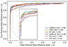 |
Fig. 1. ROC curves of six different machine learning algorithms. The inset zooms in the region from 0 to 0.05 of FPR. The AUC of each algorithm is labeled in the legend. |
To derive the best classifier, we employed the Bayesian optimization8 method to tune the hyperparameters of CatBoost. The hyperparameters and the parameter spaces used for the optimizer are listed in Table 1. The F1 score for AGNs was taken as the indicator to determine the optimal hyperparameter. The optimizer ran 100 iterations. The optimal F1 score is as high as 0.932. Other metrics and the optimal values of tuned hyperparameters are listed in Table 1.
After the hyperparameter tuning, we examined the stability of the model performance due to the random split of training and test sets. The splits of the training and test sets were randomly performed 500 times. Each time, the training set was trained by CatBoost with the optimal hyperparameters. F1 scores of both classes were then evaluated from the test set. The distributions of F1 scores for AGNs and non-AGNs are plotted in the top panel of Fig. 2. The average F1 scores for AGNs and non-AGNs are 0.905 ± 0.015 and 0.951 ± 0.008, respectively. The tuned optimal F1 score 0.932 lies at the high end of the distribution for AGNs. As a comparison, the distributions of F1 scores for CatBoost with default parameters are plotted on the bottom panel of Fig. 2. The average F1 scores are 0.910 ± 0.014 and 0.954 ± 0.007 for AGNs and non-AGNs, respectively. Small standard deviations in the F1 score distributions indicate that random splits of the training and test sets have little influence on the model training. However, the hyperparameter tuning might just select hyperparameters with a high F1 score by chance. The average F1 score derived with default hyperparameters is even better than that derived with tuned hyperparameters. Thus, in the following sections, we chose CatBoost with default hyperparameters as the best model.
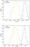 |
Fig. 2. Distribution of F1 scores for AGNs and non-AGNs with random splits of the training set and test set. The top panel was derived based on the training of CatBoost with tuned hyperparameters, while the bottom panel was derived based on the training of CatBoost with default hyperparameters. |
The threshold of the classification was also tuned with TunedThresholdClassifierCV in scikit-learn, which was set as predict_proba for the binary classification in our case. TunedThresholdClassifierCV was carried out by maximizing a metric of the classifier. The F1 score for the AGNs was again taken as the score to determine the optimal threshold. Figure 3 shows the dependence of the F1 score on the classification threshold. When the threshold is 0.5, the F1 score reaches the highest value: 0.916. Thus, the default, predict_proba = 0.5, is used through this paper. Table 2 shows the confusion matrix of the test set for the best classifier.
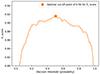 |
Fig. 3. Variation in F1 scores for AGNs along with classification thresholds. The model reaches the best F1 score 0.916 when the threshold is 0.5. |
Confusion matrix for test set of best classifier.
3.2. Application to unclassified large-area surveys
The features of our best classifier are all from AllWISE and Gaia DR3; thus, they can easily be applied to predict large samples of AGNs and non-AGNs. As we aim to identify radio AGNs, we need a large-area survey in the radio band. LoTSS DR2 uses the same high-band antenna observations of LOFAR with the LoTSS Deep field. It has a similar angular resolution but a wide sky area compared with the LoTSS Deep field, and will survey the entire northern sky in the future (Shimwell et al. 2017; Tasse et al. 2021; Shimwell et al. 2022). We cross-matched LoTSS DR2 with AllWISE and Gaia DR3 with 1″ separation. The obtained 151977 sources with all the training features in the cross-matched sample were classified by our best classifier (hereafter the prediction set). 49716 sources were classified as AGNs, and the remaining 102261 sources were classified as non-AGNs.
The WISE color-color diagram and radio/MIR excess are two of the most widely used methods of selecting radio AGNs (Hardcastle et al. 2025). In Fig. 4 the WISE color-color diagram and radio/MIR flux diagram9 of the prediction set are shown. The W3 flux density was converted from magnitude with the zero-magnitude flux density of 171.787 Jy (Jarrett et al. 2011). The predicted AGNs and non-AGN galaxies generally locate distinct regions on the WISE color-color diagram. The AGNs show a redder W1 − W2 than the non-AGNs, which follows the expectation of the emission from AGN torus. Non-AGNs occupy the regions from elliptical galaxies to SFGs (Jarrett et al. 2011).
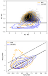 |
Fig. 4. Top panel: WISE color-color diagram for prediction set. The horizontal line presents the simple W1 − W2 criterion to select AGNs, while the gray density plots show the sources satisfying the criterion combining W1 − W2 color and W2mag (see the text for details). Bottom panel: Radio/MIR flux diagram for prediction set. The solid line shows the one-to-one correlation. The dashed line presents a division line to identify radio/MIR excess. For both panels, the orange contours represent AGNs. The levels of the contours are [10, 50, 100, 500, and 1000]. The blue contours represent non-AGNs. The levels of the contours are [10, 50, 100, 500, 1000, and 3000]. |
There are also fractional sources overlapping between AGNs and non-AGNs. Although a high completeness can be easy to achieve with a bluer W1 − W2 selection criterion, extra features besides WISE colors are needed to improve the reliability of AGN section. Assef et al. (2018) proposed two criteria to identify AGNs, which can reach a high reliability and high completeness, respectively. With the simple criterion of W1 − W2 > 0.5, they get 90% completeness of the AGN selection (C90 catalog). By combining W1 − W2 color and W2 brightness, the reliability can reach 90% (R90 catalog). For fainter sources with W2mag > 13.86, the criterion is W1 − W2 > 0.650 * exp(0.153 * (W2 − 13.86)2). For brighter sources with W2mag < 13.86, the criterion is W1 − W2 > 0.650. The C90 criterion is plotted with a horizontal black line in the top panel of Fig. 4. The AGNs classified with the R90 criterion in the prediction set are shown as the gray density plot. If the classification of our classifier is taken as the true label, the precision and recall of these two criteria in Assef et al. (2018) can be estimated. The results are shown in Table 3. As a comparison, the results for the main sample being treated as the true label are also shown. The high completeness of the C90 criterion is confirmed by the SED classification (0.891) and our classifier (0.949). The high precision of the R90 criterion for the main sample (0.936) and prediction set (0.908) indicates that our classifier can achieve a similar reliability in AGN selection with SED- and MIR-based classifications. Compared with the MIR-based criteria, our classifier can reduce the dilution of AGNs from ultraluminous infrared galaxies, and improve the completeness due to the AGNs with bluer W1 − W2 colors.
Classification Performance of two MIR Color Based Criteria.
Non-AGNs in the bottom panel of Fig. 4 are located around the line where the radio flux density equals the W3 flux density, which is similar to the known SFGs of LoTSS DR2 (Fan 2024). Most of the AGNs also show a nearly equal radio flux density with the W3 flux density, while a small fraction of AGNs exhibit obvious radio excess. For radio sources with Ftotal < FW3 + 1.5 (dashed line in the bottom panel of Fig. 4), AGNs and non-AGNs are generally undistinguishable in this plot. This indicates that the AGN selection method through radio/MIR excess would only select strong jetted AGNs but miss most of the potential radio AGNs.
4. Discussions
4.1. Dependence on multiwavelength features
Figure 5 shows the importance of training features with the permutation feature importance method (Breiman 2001), which is defined through comparing the accuracy of the test sample by permuting the features. W1 − W2 is the most important feature to identify radio AGNs, which means that permuting W1 − W2 will lead to the biggest decrease in the accuracy of the classifier. This is expected as W1 − W2 is widely used solely to identify AGNs. Besides W1 − W2, other MIR colors (W2 − W3 and W3 − W4) are also more important than optical colors to the classifier. Optical and MIR magnitudes seem unimportant in identifying radio AGNs.
 |
Fig. 5. Importance rank with permutation feature importance method. |
The performance with different combinations of optical/MIR magnitudes and colors are also compared through the metrics (precision, recall, and F1 score) of each class (Table 4). Again the differences of different combinations mainly focus on the recall and F1 score of AGNs. The performance if only MIR colors are considered is worse than that performed with MIR magnitudes. The performance improves when both MIR colors and MIR magnitudes are taken into account. Optical colors and magnitudes show a worse performance than MIR, even when MIR colors are combined with optical colors. Combining optical and MIR magnitudes achieves the second-best performance, which is next only to our best classifier, which utilizes all features.
Performance for different combinations of training features.
The SED fitting methods classify AGNs mainly by identifying the features of the torus emission at IR (Best et al. 2023). It has also been suggested that the unique MIR colors of AGNs are caused by the torus emission at different redshifts (Assef et al. 2010). Thus MIR features are no doubt important for identifying AGNs in machine learning. On the other hand, optical colors tend to identify unobscured AGNs. Obscured AGNs, who would be missed by optical features, can still be selected by MIR features. These two reasons result in worse performances for optical features than those for MIR features.
In addition, we examined the performance of the classifier for several extra features, including the radio properties and astrometric parameters (Table 4). For radio properties, we considered both the integrated radio flux density and the ratio between the radio and MIR flux density. The performance confers no improvement for either feature. The recall of AGNs decreases slightly when radio features are added. Some objects have no measurement of parallax and proper motion in the main sample. After removing the sources without these two astrometric parameters, there are 574 sources left, including 455 AGNs and 116 non-AGNs. The AGNs dominate the counts of this subsample, and perform better than non-AGNs, unsurprisingly.
4.2. Reliability of the classifier
As was mentioned in Sect. 4.1, WISE colors are the most important for our best classifier. Thus we performed a similar learning on the cross-matched sample between LoTSS Deep Fields DR1 and AllWISE with only MIR features (W1mag, W2mag, W3mag, W4mag, W1 − W2, W2 − W3, and W3 − W4). The cross-matched sample contains 1429 AGNs and 5142 non-AGNs. The precision, recall, and F1 score for AGNs are 0.794, 0.776 and 0.785, respectively. The performance is much worse than that for the main sample with the same features (Table 4). Although the colors of Gaia and the astrometric parameters seem less important to the best classifier, the Gaia detection might change the distributions of features severely after the cross-match with Gaia DR3. To clarify whether this effect would affect our classification results, we performed two independent tests.
Firstly, we examined the reliability of the classification for the prediction set in Sect. 3.2. Apart from SED fitting, the optical spectroscopy can also be used to classify quasars, AGNs, SFGs, quiescent galaxies, and stars (Bolton et al. 2012; Lyke et al. 2020). Therefore, we used the classifications in SDSS DR17 to help us examine our classification results. Except for AGNs, SDSS classified sources as galaxies and stars based on their spectra10. When the spectroscopic objects in SDSS had a class of “QSO,” or a class of “GALAXY” and a subclass containing “AGN,” they were treated as AGNs. Other sources with a class of “GALAXY” were treated as galaxies. Stars are objects with “STAR” classifications. In SDSS DR17, there are 34050 AGNs, 38017 galaxies, and 99 stars in our prediction set.
Then we compared the classification of machine learning with that of SDSS spectroscopy for the common sources. Figure 6 shows a histogram of the prediction probability of our best classifier. The orange, blue, and gray lines represent AGNs, galaxies, and stars classified by SDSS, respectively. Most SDSS AGNs have AGN probabilities in the range from 0.9 to 1.0, while galaxies have low AGN probabilities (0.0–0.1). In Table 5, we list the confusion matrix of the prediction set, in which the SDSS classifications are treated as true labels. The purity of the AGN sample can be up to 94.2 percent, while the completeness is 92.3 percent.
 |
Fig. 6. Histogram of predicted probability of being an AGN for common sources of prediction set and SDSS DR17. The orange, blue, and gray lines represent AGNs, galaxies, and stars, respectively, which are classified by SDSS. The vertical line labels the critical probability (0.5) to distinguish AGNs and non-AGNs. |
Confusion matrix when compared with SDSS classifications.
In addition, we attempted to build similar distributions (e.g., average magnitudes) of the training features between the main sample and the cross-matched sample of LoTSS Deep Fields DR1 and AllWISE. The average W2mag of the main sample is 14.20, which is brighter than 15.09 of the cross-matched sample between LoTSS Deep Fields DR1 and AllWISE. We applied a simple brightness cut with W2mag < 14.511 to the cross-matched sample of LoTSS Deep Fields DR1 and AllWISE, which results in a sample of 505 AGNs and 1164 non-AGNs with average W2mag = 13.85. The proportion between AGNs and non-AGNs is similar to that of the main sample (594:1101). CatBoost was applied to model the MIR features of this new sample. The performance of the classifier becomes much better on this sample, with precision = 0.959, recall = 0.848, and F1 = 0.900 for AGNs.
We also applied a similar magnitude cut to the cross-matched sample between LoTSS Deep Fields DR1, AllWISE, and SDSS, which contains 1106 AGNs and 4413 non-AGNs. The limiting magnitude of the GaiaG band is about 21 (Gaia Collaboration 2016; Fabricius et al. 2021), which is about 2 mag brighter than that of the SDSS g band (York et al. 2000). The average g and W2 band magnitudes of the cross-matched sample between LoTSS Deep Fields DR1, AllWISE, and SDSS are 20.54 and 14.99, respectively. We applied a magnitude cut with gmag less than 1912, which results in the average g and W2 band magnitudes brightening to 18.04 and 13.94. With the training features of MIR and optical magnitudes and colors (W1mag, W2mag, W3mag, W4mag, W1 − W2, W2 − W3, W3 − W4, umag, gmag, rmag, imag, zmag, u − g, g − r, r − i, i − z), CatBoost was again applied to the samples before and after the magnitude cut. The precision, recall, and F1 score increase to 0.969, 0.816, and 0.886 for AGNs, compared with 0.922, 0.742, and 0.822 for the sample without the magnitude cut, respectively. As the sample is severely imbalanced after the magnitude cut (157 AGNs versus 980 non-AGNs), we applied the synthetic minority oversampling technique (SMOTE) to optimize the above model with a relatively balanced training sample. For an imbalanced dataset, the metrics would be dominated by the majority class. SMOTE handles this by over-sampling the minority class (Chawla et al. 2002). The number of AGNs and non-AGNs are set to 1200 and 2000, respectively. The F1 score for AGNs increases from 0.886 to 0.909 with precision = 0.897 and recall = 0.921.
The simple magnitude cut on the above two samples shows that the distributions of training features are important to construct a well-performed classifier. Cross-matching with Gaia DR3 achieves a similar effect by selecting bright sources. Although this may change the distributions of training features, our classifier is still proven to be robust through the comparison with the spectroscopic classification of SDSS.
4.3. Classification of radio excess sources
Radio excess sources, whose radio emission is believed to be dominated by jets of AGNs, are usually identified through the excess of the radio emission produced by SF activities (Bonzini et al. 2015; Best et al. 2023; Fan 2024). There have been few attempts in the literature to identify radio excess sources with machine learning (Carvajal et al. 2023). For the main sample, we performed supervised machine learning to identify radio excess sources. The true labels were also taken from Best et al. (2023), which were classified based on the SFR estimated from SED fitting. For training features, two extra radio features, Ftotal and Ftotal/FW3, were added together with optical and MIR magnitudes and colors. CatBoost with default parameters was applied for training. Compared with the AGN classifier, classifying radio excess sources is more difficult. The precision, recall, and F1 score of radio excess sources are 0.714, 0.532, and 0.610, while they are 0.952, 0.978, and 0.965 for sources without radio excess, respectively.
Carvajal et al. (2023) performed a machine-learning-based classification for radio AGNs with features of optical and MIR photometries. Their strategy was different from that in our work. Their model was trained to clarify whether an AGN can be radio-detected, while the AGN sample was also derived from a machine-learned-based classifier. Their performance for radio detection was also worse than that for classifying AGNs.
5. Conclusions
Distinguishing AGNs from SFGs in extragalactic radio sources is important to understand the AGN feedback and evolution of galaxies. Existing methods either need costly observations, such as spectroscopy, or cannot satisfy the requirement of purity and completeness simultaneously. In this paper, we provide a supervised AGN classifier based on several large-area surveys, i.e., the LoTSS Deep Field DR1, AllWISE, and Gaia DR3. The optical/MIR photometric data from Gaia DR3 and AllWISE were collected to train the model, while the AGN and non-AGN classifications based on SED fitting were treated as the true labels. To select the optimal learning algorithms, the F1 score and ROC curve were compared among six algorithms. Then the optimal hyperparameters of the best algorithm were determined through the hyperparameter tuning and the stability of model performance. Finally, CatBoost with its default hyperparameters was chosen to build the best classifier.
We also compared model performance for different training features and different datasets. The best performance is achieved when all the optical and MIR magnitude and colors are combined. Although MIR features appear to be more important than optical features, the model performance gets worse if only MIR features are considered. Including radio and astrometric features results in no improvement in the model performance. The performance with different cross-matched samples confirms that the distributions of train features can also affect the model performance. Uniform model performance can be obtained if the average magnitudes of different training samples are adjusted to be similar.
Our best classifier achieves both high purity and completeness in identifying AGNs, with precision = 0.974, recall = 0.865, and F1 = 0.916. Compared with AGN classification methods based on color-color diagram and radio/MIR excess, our classifier could improve the completeness by selecting AGNs with blue MIR colors and weak radio emission, and improve the purity by excluding non-AGNs with red MIR colors. This classifier was then applied to classify radio sources in the cross-matched sample of LoTSS DR2, AllWISE, and Gaia DR3. A sample of 49716 AGNs and 102261 non-AGNs was derived. The reliability of the machine-learning-based classification was verified by comparing it with the spectroscopic classification of SDSS DR17. The purity and completeness for AGN classification can be as high as 94.2 percent and 92.3 percent, respectively. With just the training features from AllWISE and Gaia, our classifier can easily be applied to select and analyze radio AGNs in other radio surveys.
We also built a classifier to identify radio excess sources. The performance is much worse than that for AGN classification, with precision = 0.714, recall = 0.532, and F1 = 0.610.
Hardcastle et al. (2023) presented redshift estimations for more than half of radio sources in LoTSS DR2. Combining the redshift and source extension information in Hardcastle et al. (2023), one can estimate the fraction of resolved radio sources for different redshift bins. The fraction decreases from 34%, 19% to 7% for the redshift bins [< 0.01], [0.01, 0.1] and [> 0.1], respectively.
Actually, both SFGs and LERGs are included in non-AGN sample. A four-class classifier should be more suitable to distinguish radio sources with different properties. However, LERGs (61) and HERGs (91) are few in the main sample. More importantly, the four-class can be exactly inferred combining AGN classification and radio excess classification. Thus building two binary class classifiers is also adequate. We will discuss the classifier on radio excess sources in Sect. 4.3.
Some of machine learning algorithms can handle null values, such as RF, HGBT and CatBoost. We apply the default mode for null values of CatBoost with the 3034 objects in the original cross-matching sample, where the missing values are processed as the minimum value. The performance of the classifier changes slightly compared with our best classifier (Sect. 3.1), with the F1 = 0.899 and 0.957 for AGNs and non-AGNs.
Overfitting problem of HGBT can be reduced by enabling early stopping or by reducing the maximum number of iterations. With max_iter = 30, the accuracy for the training set decreases to 0.981. Meanwhile, a higher F1 score of 0.916 is derived, which is close to the results of CatBoost. As we just select the optimal algorithm with its default parameters, CatBoost is chosen to construct the best classifier in the following section.
The behaviors of the radio/MIR flux diagram for all four WISE bands are similar, except that the overall MIR flux density increases from W1 to W4 band. As MIR emission of W3 band is usually suggested to distinguish radio AGNs from radio SFGs (Fan 2024; Hardcastle et al. 2025), or as an indicator of SFRs (Cluver et al. 2017) in the literature, only the plot between radio and W3 flux density is shown in this paper.
This criterion is firstly determined in order to match the average W2mag of the main sample. When the criterion is taken as 15.0, the average W2mag is 14.23, which is closest to 14.20 of the main sample. The classifier gets a F1 score 0.849 for AGNs. Then we attempt to maximize the F1 score. The criterion changes from 14.4 to 15.1 with a step of 0.1 mag. F1 score for AGNs shows the lowest value of 0.847 at 15.1 mag, and shows the highest value of 0.900 at 14.5 mag.
This criterion is determined to match the difference on the limiting magnitude between Gaia and SDSS surveys, which is about 2 magnitudes on the mean magnitude. For a criterion of 19.5, the average g band magnitude is 18.42, which is closest to target value of 18.54. The F1 score for AGNs is also maximized by changing the criterion from 18.5 to 20.0 with a step of 0.5 mag. The best F1 score is 0.886 for the criterion of 19.0, while the worst one is 0.756 for the criterion of 18.5.
Acknowledgments
We thank the anonymous referee for constructive comments which improve the paper greatly. This research is funded by National Natural Science Foundation of China (NSFC; grant No. 12003014). This publication makes use of data products from LOFAR. LOFAR data products were provided by the LOFAR Surveys Key Science project (LSKSP; https://lofar-surveys.org/) and were derived from observations with the International LOFAR Telescope (ILT). LOFAR (van Haarlem et al. 2013) is the Low Frequency Array designed and constructed by ASTRON. It has observing, data processing, and data storage facilities in several countries, which are owned by various parties (each with their own funding sources), and which are collectively operated by the ILT foundation under a joint scientific policy. The efforts of the LSKSP have benefited from funding from the European Research Council, NOVA, NWO, CNRS-INSU, the SURF Cooperative, the UK Science and Technology Funding Council and the Jülich Supercomputing Centre. This publication makes use of data products from the Wide-field Infrared Survey Explorer, which is a joint project of the University of California, Los Angeles, and the Jet Propulsion Laboratory/California Institute of Technology, funded by the National Aeronautics and Space Administration. This work has made use of data from the European Space Agency (ESA) mission Gaia (https://www.cosmos.esa.int/gaia), processed by the Gaia Data Processing and Analysis Consortium (DPAC, https://www.cosmos.esa.int/web/gaia/dpac/consortium). Funding for the DPAC has been provided by national institutions, in particular the institutions participating in the Gaia Multilateral Agreement. This research has made use of the VizieR catalog access tool, CDS, Strasbourg, France (Ochsenbein 1996). The original description of the VizieR service was published in Ochsenbein et al. (2000).
References
- Abdurro’uf, Accetta, K., Aerts, C., et al. 2022, ApJS, 259, 35 [NASA ADS] [CrossRef] [Google Scholar]
- Assef, R. J., Kochanek, C. S., Brodwin, M., et al. 2010, ApJ, 713, 970 [NASA ADS] [CrossRef] [Google Scholar]
- Assef, R. J., Stern, D., Kochanek, C. S., et al. 2013, ApJ, 772, 26 [Google Scholar]
- Assef, R. J., Stern, D., Noirot, G., et al. 2018, ApJS, 234, 23 [Google Scholar]
- Baldwin, J. A., Phillips, M. M., & Terlevich, R. 1981, PASP, 93, 5 [Google Scholar]
- Ball, N. M., & Brunner, R. J. 2010, Int. J. Mod. Phys. D, 19, 1049 [Google Scholar]
- Baron, D. 2019, arXiv e-prints [arXiv:1904.07248] [Google Scholar]
- Best, P. N., & Heckman, T. M. 2012, MNRAS, 421, 1569 [NASA ADS] [CrossRef] [Google Scholar]
- Best, P. N., Kondapally, R., Williams, W. L., et al. 2023, MNRAS, 523, 1729 [NASA ADS] [CrossRef] [Google Scholar]
- Blandford, R., Meier, D., & Readhead, A. 2019, ARA&A, 57, 467 [NASA ADS] [CrossRef] [Google Scholar]
- Bolton, A. S., Schlegel, D. J., Aubourg, É., et al. 2012, AJ, 144, 144 [NASA ADS] [CrossRef] [Google Scholar]
- Bonzini, M., Mainieri, V., Padovani, P., et al. 2015, MNRAS, 453, 1079 [Google Scholar]
- Boucaud, A., Huertas-Company, M., Heneka, C., et al. 2020, MNRAS, 491, 2481 [Google Scholar]
- Bradley, A. P. 1997, Pattern Recognit., 30, 1145 [Google Scholar]
- Breiman, L. 2001, Mach. Learn., 45, 5 [Google Scholar]
- Busca, N., & Balland, C. 2018, MMRAS, submitted, [arXiv:1808.09955] [Google Scholar]
- Carliles, S., Budavári, T., Heinis, S., Priebe, C., & Szalay, A. S. 2010, ApJ, 712, 511 [NASA ADS] [CrossRef] [Google Scholar]
- Carvajal, R., Matute, I., Afonso, J., et al. 2023, A&A, 679, A101 [NASA ADS] [CrossRef] [EDP Sciences] [Google Scholar]
- Chawla, N. V., Bowyer, K. W., Hall, L. O., & Kegelmeyer, W. P. 2002, J. Artif. Intell. Res., 16, 321 [CrossRef] [Google Scholar]
- Clarke, A. O., Scaife, A. M. M., Greenhalgh, R., & Griguta, V. 2020, A&A, 639, A84 [NASA ADS] [CrossRef] [EDP Sciences] [Google Scholar]
- Cluver, M. E., Jarrett, T. H., Dale, D. A., et al. 2017, ApJ, 850, 68 [Google Scholar]
- Cutri, R. M., Wright, E. L., Conrow, T., et al. 2021, VizieR On-line Data Catalog: II/328 [Google Scholar]
- Dai, Y., Xu, J., Song, J., et al. 2023, ApJS, 268, 34 [NASA ADS] [CrossRef] [Google Scholar]
- Euclid Collaboration (Bisigello, L., et al.) 2024, A&A, 691, A1 [NASA ADS] [CrossRef] [EDP Sciences] [Google Scholar]
- Fabricius, C., Luri, X., Arenou, F., et al. 2021, A&A, 649, A5 [NASA ADS] [CrossRef] [EDP Sciences] [Google Scholar]
- Faisst, A. L., Prakash, A., Capak, P. L., & Lee, B. 2019, ApJ, 881, L9 [NASA ADS] [CrossRef] [Google Scholar]
- Fan, X.-L. 2024, ApJ, 966, 53 [Google Scholar]
- Feigelson, E. D., de Souza, R. S., Ishida, E. E. O., & Jogesh Babu, G. 2021, Ann. Rev. Stat. Appl., 8, 493 [Google Scholar]
- Fotopoulou, S. 2024, Astron. Comput., 48, 100851 [Google Scholar]
- Fu, Y., Wu, X.-B., Li, Y., et al. 2024, ApJS, 271, 54 [NASA ADS] [CrossRef] [Google Scholar]
- Gaia Collaboration (Prusti, T., et al.) 2016, A&A, 595, A1 [NASA ADS] [CrossRef] [EDP Sciences] [Google Scholar]
- Gaia Collaboration (Bailer-Jones, C. A. L., et al.) 2023a, A&A, 674, A41 [NASA ADS] [CrossRef] [EDP Sciences] [Google Scholar]
- Gaia Collaboration (Vallenari, A., et al.) 2023b, A&A, 674, A1 [NASA ADS] [CrossRef] [EDP Sciences] [Google Scholar]
- Glauch, T., Kerscher, T., & Giommi, P. 2022, Astron. Comput., 41, 100646 [NASA ADS] [CrossRef] [Google Scholar]
- Guo, Z., Wu, J. F., & Sharon, C. E. 2022, NeurIPS conference ML4PS workshop, arXiv e-prints [arXiv:2212.07881] [Google Scholar]
- Hardcastle, M. J., Horton, M. A., Williams, W. L., et al. 2023, A&A, 678, A151 [NASA ADS] [CrossRef] [EDP Sciences] [Google Scholar]
- Hardcastle, M. J., Pierce, J. C. S., Duncan, K. J., et al. 2025, MNRAS, 539, 1856 [Google Scholar]
- Heintz, K. E., Fynbo, J. P. U., Høg, E., et al. 2018, A&A, 615, L8 [NASA ADS] [CrossRef] [EDP Sciences] [Google Scholar]
- Ho, L. C. 2008, ARA&A, 46, 475 [Google Scholar]
- Ivezić, Ž., Connolly, A. J., VanderPlas, J. T., & Gray, A. 2014, Statistics, Data Mining, and Machine Learning in Astronomy (A Practical Python Guide for the Analysis of Survey Data) [Google Scholar]
- Jarrett, T. H., Cohen, M., Masci, F., et al. 2011, ApJ, 735, 112 [Google Scholar]
- Kang, S.-J., Fan, J.-H., Mao, W., et al. 2019, ApJ, 872, 189 [NASA ADS] [CrossRef] [Google Scholar]
- Karsten, J., Wang, L., Margalef-Bentabol, B., et al. 2023, A&A, 675, A159 [NASA ADS] [CrossRef] [EDP Sciences] [Google Scholar]
- Kellermann, K. I., Sramek, R., Schmidt, M., Shaffer, D. B., & Green, R. 1989, AJ, 98, 1195 [Google Scholar]
- Kondapally, R., Best, P. N., Hardcastle, M. J., et al. 2021, A&A, 648, A3 [EDP Sciences] [Google Scholar]
- Kuntzer, T., Tewes, M., & Courbin, F. 2016, A&A, 591, A54 [NASA ADS] [CrossRef] [EDP Sciences] [Google Scholar]
- Lao, B., Jaiswal, S., Zhao, Z., et al. 2023, Astron. Comput., 44, 100728 [Google Scholar]
- Lin, J. Y.-Y., Pandya, S., Pratap, D., et al. 2023, MNRAS, 518, 4921 [Google Scholar]
- Lochner, M., McEwen, J. D., Peiris, H. V., Lahav, O., & Winter, M. K. 2016, ApJS, 225, 31 [NASA ADS] [CrossRef] [Google Scholar]
- Lyke, B. W., Higley, A. N., McLane, J. N., et al. 2020, ApJS, 250, 8 [NASA ADS] [CrossRef] [Google Scholar]
- Ma, Z., Xu, H., Zhu, J., et al. 2019, ApJS, 240, 34 [NASA ADS] [CrossRef] [Google Scholar]
- Magliocchetti, M. 2022, A&A Rev., 30, 6 [NASA ADS] [CrossRef] [Google Scholar]
- Mateos, S., Alonso-Herrero, A., Carrera, F. J., et al. 2012, MNRAS, 426, 3271 [Google Scholar]
- McLaughlin, S. A. J., Mullaney, J. R., & Littlefair, S. P. 2024, MNRAS, 529, 2877 [Google Scholar]
- Morabito, L. K., Sweijen, F., Radcliffe, J. F., et al. 2022, MNRAS, 515, 5758 [NASA ADS] [CrossRef] [Google Scholar]
- Ochsenbein, F. 1996, The VizieR database of astronomical catalogues, CDS, Centre de Données astronomiques de Strasbourg [Google Scholar]
- Ochsenbein, F., Bauer, P., Marcout, J., et al. 2000, A&AS, 143, 23 [NASA ADS] [CrossRef] [EDP Sciences] [Google Scholar]
- Pacifici, C., Iyer, K. G., Mobasher, B., et al. 2023, ApJ, 944, 141 [NASA ADS] [CrossRef] [Google Scholar]
- Padovani, P. 2016, A&ARv, 24, 13 [Google Scholar]
- Panessa, F., Baldi, R. D., Laor, A., et al. 2019, Nat. Astron., 3, 387 [Google Scholar]
- Pedregosa, F., Varoquaux, G., Gramfort, A., et al. 2011, J. Mach. Learn. Res., 12, 2825 [Google Scholar]
- Peterson, B. M. 1997, An Introduction to Active Galactic Nuclei (Cambridge: New York Cambridge University Press) [Google Scholar]
- Prokhorenkova, L., Gusev, G., Vorobev, A., Veronika Dorogush, A., & Gulin, A. 2017, arXiv e-prints [arXiv:1706.09516] [Google Scholar]
- Richards, J. W., Starr, D. L., Butler, N. R., et al. 2011, ApJ, 733, 10 [NASA ADS] [CrossRef] [Google Scholar]
- Sabater, J., Best, P. N., Tasse, C., et al. 2021, A&A, 648, A2 [EDP Sciences] [Google Scholar]
- Shimwell, T. W., Röttgering, H. J. A., Best, P. N., et al. 2017, A&A, 598, A104 [NASA ADS] [CrossRef] [EDP Sciences] [Google Scholar]
- Shimwell, T. W., Hardcastle, M. J., Tasse, C., et al. 2022, A&A, 659, A1 [NASA ADS] [CrossRef] [EDP Sciences] [Google Scholar]
- Shu, Y., Koposov, S. E., Evans, N. W., et al. 2019, MNRAS, 489, 4741 [Google Scholar]
- Stern, D., Assef, R. J., Benford, D. J., et al. 2012, ApJ, 753, 30 [Google Scholar]
- Tardugno Poleo, V., Finkelstein, S. L., Leung, G., et al. 2023, AJ, 165, 153 [NASA ADS] [CrossRef] [Google Scholar]
- Tasse, C., Shimwell, T., Hardcastle, M. J., et al. 2021, A&A, 648, A1 [EDP Sciences] [Google Scholar]
- Taylor, M. B. 2005, in Astronomical Data Analysis Software and Systems XIV, eds. P. Shopbell, M. Britton, & R. Ebert, ASP Conf. Ser., 347, 29 [Google Scholar]
- Ulvestad, J. S., Antonucci, R. R. J., & Barvainis, R. 2005, ApJ, 621, 123 [Google Scholar]
- van Haarlem, M. P., Wise, M. W., Gunst, A. W., et al. 2013, A&A, 556, A2 [NASA ADS] [CrossRef] [EDP Sciences] [Google Scholar]
- Veronika Dorogush, A., Ershov, V., & Gulin, A. 2018, arXiv e-prints [arXiv:1810.11363] [Google Scholar]
- Wang, A., An, T., Cheng, X., et al. 2023, MNRAS, 518, 39 [Google Scholar]
- Wright, E. L., Eisenhardt, P. R. M., Mainzer, A. K., et al. 2010, AJ, 140, 1868 [Google Scholar]
- Yao, H. F. M., Cluver, M. E., Jarrett, T. H., et al. 2022, ApJ, 939, 26 [NASA ADS] [CrossRef] [Google Scholar]
- York, D. G., Adelman, J., Anderson, J. E. Jr, et al. 2000, AJ, 120, 1579 [Google Scholar]
- Zeraatgari, F. Z., Hafezianzadeh, F., Zhang, Y. X., Mosallanezhad, A., & Zhang, J. Y. 2024, A&A, 688, A33 [NASA ADS] [CrossRef] [EDP Sciences] [Google Scholar]
All Tables
Hyperparameters and model performance for different machine learning algorithms.
All Figures
|
Fig. 1. ROC curves of six different machine learning algorithms. The inset zooms in the region from 0 to 0.05 of FPR. The AUC of each algorithm is labeled in the legend. |
| In the text | |
|
Fig. 2. Distribution of F1 scores for AGNs and non-AGNs with random splits of the training set and test set. The top panel was derived based on the training of CatBoost with tuned hyperparameters, while the bottom panel was derived based on the training of CatBoost with default hyperparameters. |
| In the text | |
|
Fig. 3. Variation in F1 scores for AGNs along with classification thresholds. The model reaches the best F1 score 0.916 when the threshold is 0.5. |
| In the text | |
|
Fig. 4. Top panel: WISE color-color diagram for prediction set. The horizontal line presents the simple W1 − W2 criterion to select AGNs, while the gray density plots show the sources satisfying the criterion combining W1 − W2 color and W2mag (see the text for details). Bottom panel: Radio/MIR flux diagram for prediction set. The solid line shows the one-to-one correlation. The dashed line presents a division line to identify radio/MIR excess. For both panels, the orange contours represent AGNs. The levels of the contours are [10, 50, 100, 500, and 1000]. The blue contours represent non-AGNs. The levels of the contours are [10, 50, 100, 500, 1000, and 3000]. |
| In the text | |
|
Fig. 5. Importance rank with permutation feature importance method. |
| In the text | |
|
Fig. 6. Histogram of predicted probability of being an AGN for common sources of prediction set and SDSS DR17. The orange, blue, and gray lines represent AGNs, galaxies, and stars, respectively, which are classified by SDSS. The vertical line labels the critical probability (0.5) to distinguish AGNs and non-AGNs. |
| In the text | |
Current usage metrics show cumulative count of Article Views (full-text article views including HTML views, PDF and ePub downloads, according to the available data) and Abstracts Views on Vision4Press platform.
Data correspond to usage on the plateform after 2015. The current usage metrics is available 48-96 hours after online publication and is updated daily on week days.
Initial download of the metrics may take a while.