| Issue |
A&A
Volume 701, September 2025
|
|
|---|---|---|
| Article Number | A178 | |
| Number of page(s) | 9 | |
| Section | Extragalactic astronomy | |
| DOI | https://doi.org/10.1051/0004-6361/202553744 | |
| Published online | 12 September 2025 | |
The effect of environment on the mass assembly history of the Milky Way and M31
1
Kapteyn Astronomical Institute, University of Groningen, P.O Box 800 9700 AV Groningen, The Netherlands
2
Max-Planck-Institut für Astrophysik, Karl-Schwarzschild-Straße 1, 85748 Garching, Germany
3
The Oskar Klein Centre, Department of Physics, Stockholm University, Albanova University Center, SE 106 91 Stockholm, Sweden
4
CNRS & Sorbonne Université, UMR 7095, Institut d’Astrophysique de Paris, 98 bis boulevard Arago, F-75014 Paris, France
⋆ Corresponding author: This email address is being protected from spambots. You need JavaScript enabled to view it.
Received:
13
January
2025
Accepted:
25
June
2025
Abstract
We study the mass growth histories of the haloes of Milky Way and M31 analogues formed in constrained cosmological simulations of the Local Group. These gravity-only simulations constitute a fair and representative set of Λ cold dark matter (ΛCDM) realisations conditioned on the masses, positions, and relative velocities of the two big haloes and on the observed recession velocities at the positions of nearby isolated galaxies. Our M31 haloes have similar mass growth histories as the isolated analogues in the TNG dark-matter-only simulations, while our Milky Ways typically form earlier, with suppressed growth at late times. On average, our Milky Ways assemble half their halo mass by ⟨z50⟩ = 1.4 and our M31s by ⟨z50⟩ = 1.2, whereas ⟨z50⟩ = 1.1 for their isolated analogues. Mass growth associated with major and minor mergers is also biased early for the Milky Way in comparison to M31. Most accretion occurs 1–4 Gyr after the Big Bang; growth at later times is relatively quiescent. Based on the mass ratio and time of infall, we find that 32% of our Milky Ways experienced a Gaia-Enceladus-Sausage-like merger, 13% host a massive Large Magellanic Cloud-like satellite at the present day, and 5% have both. In one case, a Small Magellanic Cloud analogue and a Sagittarius analogue are also present, showing that the most important mergers of the Milky Way can be reproduced in its Local Group environment in ΛCDM. We find that the material that makes up the Milky Way and M31 haloes at the present day initially collapsed onto a plane roughly aligned with the Local Sheet and super-galactic plane; after z ∼ 2, accretion occurred mostly within this plane, with the tidal effects of the heavier companion, M31, significantly impacting the late growth history of the Milky Way.
Key words: galaxies: evolution / galaxies: formation / Local Group / dark matter
© The Authors 2025
 Open Access article, published by EDP Sciences, under the terms of the Creative Commons Attribution License (https://creativecommons.org/licenses/by/4.0), which permits unrestricted use, distribution, and reproduction in any medium, provided the original work is properly cited.
This article is published in open access under the Subscribe to Open model. This email address is being protected from spambots. You need JavaScript enabled to view it. to support open access publication.
1. Introduction
In recent years, tremendous progress has been made on constraining the assembly history of the Milky Way (MW) using Gaia data (Gaia Collaboration 2018, 2023) in combination with ground-based spectroscopic surveys such as APOGEE (Majewski et al. 2017). We now know that the Galaxy experienced its last major merger (LMM) approximately 10 Gyr ago, with a system dubbed Gaia-Enceladus (Helmi et al. 2018); this created a kinematic structure known as the Gaia-Sausage (Belokurov et al. 2018), and hence the event is often referred to as the Gaia-Enceladus-Sausage (GES). We also know that since then accretion has been primarily driven by minor mergers (Helmi 2020; Naidu et al. 2020; Deason & Belokurov 2024).
This relatively quiescent recent merger history has implications for key properties of the MW. For instance, it is consistent, and perhaps even necessary for the preservation of its thin, kinematically cold disc, which could be disrupted or thickened by a significant late merger (Toth & Ostriker 1992; Stewart et al. 2008). That said, recent hydrodynamical simulations suggest that thin discs can reform quickly even after a major merger if sufficient gas is available (Sotillo-Ramos et al. 2022). The LMM may also have influenced the chemo-dynamical properties of the Galaxy (e.g. Buck 2020; Buck et al. 2023; Renaud et al. 2021; Ciucă et al. 2024). Such a quiescent assembly also raises questions about how typical the MW is within the standard Λ cold dark matter (ΛCDM) model, with some studies suggesting the MW is an outlier with respect to other local spirals (Hammer et al. 2007).
The idea that the MW is a typical L* galaxy may also be challenged by the presence of two bright satellites, the Large and Small Magellanic Clouds (LMC and SMC, respectively). Observationally, such systems are uncommon; for example, Liu et al. (2011) found only 11% of their SDSS sample of MW-like galaxies to have a satellite of similar luminosity to the LMC, with only 3.5% having analogues of both clouds. More recently, in the SAGA survey (Mao et al. 2024) a third of the MW-like galaxies contain an LMC-mass satellite, and these systems often have richer satellite populations than the MW. Cosmological simulations also produce relatively few MW-mass haloes with sub-haloes massive enough to host the LMC and SMC (Boylan-Kolchin et al. 2011; Busha et al. 2011; Boylan-Kolchin et al. 2012).
There have been several recent attempts to estimate the likelihood of a MW-like halo experiencing a GES-like merger and simultaneously hosting massive satellites like the Magellanic Clouds. These studies have been carried out on large suites of dark-matter-only (DMO) and hydrodynamical simulations. For example, Evans et al. (2020) find that 5% of MW-mass haloes in the EAGLE simulations (Schaye et al. 2015) have a GES-like event and then no merger with an equally massive object after z = 1, while 16% have an LMC analogue at the present day; only 0.65% satisfy the two constraints simultaneously. The halo progenitors of these 0.65% of haloes appear to be much less massive than the average at early times (before the merger with the GES). In more recent work, Buch et al. (2024) searched cosmological DMO simulations for MW-like haloes that have both a GES-like event at early times and an LMC analogue at late times. Depending on the exact requirements, as few as 0.75% of all MW candidates were acceptable, of which only a small subset were in a group-like environment.
An important factor, often neglected in searches for MW analogues, may be the specific cosmic environment. While many papers consider relatively isolated systems, the real MW is part of the Local Group (LG) and has a massive companion (M31). The immediate surroundings of the LG may also influence galaxy assembly in a significant way. For instance, Santos-Santos et al. (2021) find that LMC-like satellites are about twice as likely around LG analogues in the APOSTLE simulations as around isolated galaxies (Sawala et al. 2016; Fattahi et al. 2016). Earlier assembly was also found in the constrained simulations of LG formation of Carlesi et al. (2020) and in the three LG analogues found by Santistevan et al. (2020) in their FIRE-2 hydrodynamical simulations. These studies all suggest that a proper understanding of the MW’s assembly history, and whether it is unusual, requires accounting for the LG context.
We studied the effect of environment on the mass assembly history of the MW (in particular, its embedding in the LG, of which it is not the most massive member) using the constrained simulations presented in Wempe et al. (2024, hereafter W24). By using a suite of simulations that match the detailed properties of the LG, we aim to understand whether the MW is expected to assemble early and how its environment has affected its growth history.
2. Methodology
2.1. W24 Local Group simulations
The constrained LG simulations presented in W24 constitute a fair and representative set of ΛCDM realisations conditional on properties of the LG; specifically, they are constrained to match the masses, positions and 3D velocities of the MW-M31 pair, and are also constrained by the observed velocity field within ∼4 Mpc. Hence, if we compare these simulations with MW-mass or M31-mass galaxies identified in large cosmological simulations of random volumes, we can quantify the effect of their specific environment on the MW and M31 mass assembly histories.
For this work, we extracted a set of 224 LG realisations1 from the chains2 run in W24. For each sample, we took the initial condition field, added random small-scale perturbations at scales below those included in the chain simulations, and generated initial conditions at redshift z = 633 We describe the exact procedure for the up-sampling of the initial conditions in Appendix A. We then integrated these initial conditions to z = 0 using Gadget-4 (Springel et al. 2021). The numerical parameters used in the gravity-only simulations are summarised in Table 1. Although the resolution of our re-simulations is relatively low, it is comparable to that of the Millennium-II simulation by Boylan-Kolchin et al. (2009, 2010); who demonstrated convergence for MW-mass halo growth histories by comparing to the higher resolution Aquarius level-2 simulation suite from Springel et al. (2008).
Numerical parameters used in the LG Gadget-4 simulations presented in this paper.
We used the friends-of-friends (FoF) group-finder, SUBFIND-HBT, and merger tree implementations bundled with Gadget-4 to obtain the group catalogues, sub-halo catalogues, and the merger trees, respectively. In this paper, we denote the virial mass as M200c and define it as the mass within a sphere of average density 200ρc, where ρc is the critical density of the Universe4. The virial masses for the Milky Way and M31 DM haloes are  and
and  (mean and 16th and 84th percentiles) As stated earlier, our MW and M31 haloes are constructed to match the observational constraints, with their masses reproduced within observational uncertainties in our posterior simulations with Gadget. The distances between the main haloes are
  kpc, they are infalling with radial velocities of
  , and have tangential velocities of
  . The spread in these quantities, especially the radial velocity and distance, is larger than the scatter in the low-resolution runs presented in W24. This is caused by the (significant) increase in resolution of the re-simulations, as well as the added entropy resulting from the augmenting of initial conditions with small-scale random fluctuations.
2.2. IllustrisTNG MW- and M31-mass haloes
To assess the effect of the Large Group environment, we compared our haloes with a sample of isolated MW- and M31-mass haloes extracted from the DMO variant of TNG50 (Nelson et al. 2019a,b; Pillepich et al. 2019). We extracted two subsets of the sub-halo catalogue to represent, respectively, MW-mass and M31-mass samples. For this, we required that the M200c values, centred on the position of the main sub-halo’s most bound particle, be within 1σ of the masses of the MW and M31 analogues in the W24 sample. In practice, this means M200c,MW ∈ (0.98 − 1.45) × 1012 M⊙ and M200c,M31 ∈ (1.62 − 2.52) × M⊙. Additionally, we required there to be no sub-halo of more than half the mass of the primary halo within 1 Mpc. This resulted in 52 isolated MW-mass and 53 isolated M31-mass haloes from TNG50-DMO. Because of the isolation criterion, all sub-haloes in our sample are the main sub-halo of their respective FoF group5. These samples are similar to, and mostly a subset of the ‘halo-based’ selection of MW/M31-mass galaxies (also from TNG50) by Pillepich et al. (2024), who selected the central sub-haloes of FoF groups with masses between 6 × 10¹¹M⊙ and 2 × 10¹² M⊙. The only notable differences are the mass ranges (e.g. some of our M31-mass haloes are not present in their sample due to their 2 × 10¹² M⊙ upper limit), and that their sample was built on the full-physics version of TNG50 instead of TNG50-DMO.
We mostly used the Sublink merger trees part of TNG50’s public data release (Nelson et al. 2019b). This algorithm differs from the one used for the merger trees for the constrained LG simulations; however, the only quantity we used is the position of the most bound particle, which should be robust for the MW and M31 main progenitors across different sub-halo finders and linkers. Nonetheless, we found that for ∼10% of objects, these merger trees missed a link in the main progenitor branch. We therefore decided to perform an additional correction step: if the sum of the progenitor masses of a particular sub-halo in the tree is less than half of the mass of the descendant (meaning it misses a massive progenitor), we searched in the neighbouring (comoving) 200 kpc for a sub-halo with a similar mass and, if found, manually added it to the merger tree. We verified via visual inspection of the snapshots that in all 22 such cases, the manually inserted extra link looked robust and that no wrong sub-haloes have been linked.
3. Results
3.1. Mass assembly history
We show the evolution of the virial mass M200c of the MW/M31 haloes in Fig. 1. In the top-left panel, we plot the mass growth history normalised by the present-day mass in the constrained simulations. This figure shows that on average the MW assembles a bit earlier than M31 in our simulations. Some of this bias towards early assembly could in principle be attributed to the MW being less massive (the ratio of the two virial masses is  in our suite) since, on average, heavier objects have a later assembly time in ΛCDM.
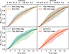 |
Fig. 1. Comparison of the mass growth histories of the MW and M31 galaxies from the constrained simulations of W24, compared to random MW- or M31-mass galaxies from TNG50-DMO. The central lines are the means, and shading indicates the 16–84 percentile regions. The un-normalised mass growth histories are shown in Appendix C. |
To analyse this finding in more depth, we considered the mass histories of MW- and M31-mass haloes from the TNG50 DMO variant, selected as described above. The top-right panel of Fig. 1 compares their mass growth histories; random MW-mass haloes indeed assemble slightly earlier on average. However, the amplitude of the effect is not enough to explain what is seen for our constrained simulations in the top-left panel. Furthermore, comparing the MW growth histories of the constrained realisation and the TNG samples (bottom-left panel), we see that the former are biased towards earlier assembly (although well within the spread), while for M31 the effect of the environment is not apparent, as shown in the bottom-right panel. In summary, it appears that the LG environment causes MW haloes to grow slightly faster at early times and more slowly at late times compared to their isolated counterparts. It also results in much less scatter in the allowed histories of the MW compared to the TNG sample of MWs. In particular, the tail of late-forming MWs that are present in the TNG sample is absent in our LG sample.
The distributions of the redshift at which 50% of the mass was attained, z50, plotted in Fig. 2, support a similar view. In this figure, the top panel corresponds to the MWs and their comparison sample, and the bottom to the M31s. In 60% of cases z50 is larger (zX is defined as the redshift at which X% of the present-day mass was in place), and in 69% z10 is larger, although the magnitude of the difference is ≲1σ of the scatter betweenrealisations.
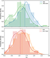 |
Fig. 2. Distribution of the redshifts at which half the final mass was accumulated (z50) for the constrained MW and M31 haloes, compared to the random MW- or M31-mass haloes from TNG50-DMO. |
The mass growth history is at least in part driven by mergers and accretion events. In Fig. 3 we show the average mass accretion rates via mergers for our MWs as a function of mass ratio and infall time, as well as the difference between our MWs and M31s. The mass ratio is defined as the ratio of sub-halo to most massive progenitor mass when the sub-halo reaches its maximum mass, while the infall time refers to when the sub-halo first becomes part of the FoF group of the main halo’s progenitor. For the MWs, 52% of the total mass accretion can be attributed to mass bound to merging objects at some point in time, compared to 55% for M31. The remainder comes from unresolved mergers and smooth accretion. Our MWs exhibit a sharp peak in merger-associated mass accretion at early times, followed by a steep decline after the third bin at an infall time of 4 Gyr. In the difference plot on the right, this is reflected in the higher normalised mass accretion in the first three bins compared to our M31s. Conversely, at times later than 4 Gyr, the M31s display more accretion from both major and minor mergers, indicating that our MWs generally have a quieter recent merger history than our M31s. Quantitatively, when combining all infall events across our MWs and M31s, the median infall time of mass associated with major mergers (mass ratio μ > 0.25) is at t50, μ > 0.25 = 3.3 Gyr, which is 0.4 Gyr earlier than for the M31s (t50, μ > 0.25 = 3.7 Gyr). Similarly, the median infall time for minor mergers (0.1 < μ < 0.25) is t50, 0.1 < μ < 0.25 = 3.6 Gyr for the MWs, which is 0.7 Gyr earlier than for the M31 analogues (t50, 0.1 < μ < 0.25 = 4.3 Gyr). The bootstrap errors, estimated by resampling the merger events, are less than 0.16 Gyr, making the differences significant to 2.4σ for major mergers and 4.7σ for minor mergers. We also examined the time of the LMM (with mass ratio μ > 0.25) of our MWs and M31s. The average time of the LMM (μ > 0.25) shows no significant difference between the two haloes: the MWs have an average tLMM of 3.13 Gyr while the M31s have 3.15 Gyr. However, tLMM is a rather stochastic quantity, with a large simulation-to-simulation scatter of 2 Gyr, which could obscure any small signal.
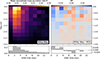 |
Fig. 3. Merger-associated mass accretion rates as a function of infall time and mass ratio (μ). For each bin, the peak masses of the infalling objects are summed and normalised by the total merger-associated mass accretion for the respective halo (MW or M31). This normalised mass accretion rate (R) is then averaged over simulations, with the resulting values shown by the colours. Left panel: This quantity for the MW. Right panel: Difference between the MW and M31. The histograms at the bottom represent the same quantity but marginalised over mass ratio, showing the 1D distribution as a function of infall time. |
We next identified GES-like mergers, which we defined as those satisfying the following criteria: (1) it is the last merger and had a mass ratio μ > 0.2; (2) the object was fully destroyed [2,6] Gyr after the Big Bang; and (3) the mass ratio is 0.2 < μ < 0.5. These criteria reflect our understanding of GES as the LMM of the MW, including its accretion time (e.g. Helmi 2020, and references therein), where we allow for substantial offset due to observational uncertainties as well as those stemming from extrapolating from gravity-only simulations. With these criteria we find that 72 out of our 224 simulations have such a merger.
Since the behaviour at late times is also interesting, we also searched for an LMC-like object, which we define as follows: (1) the LMC-sub-halo is the most massive at the present day; (2) it first crossed the MW’s r200c more than 0.5 Gyr ago; (3) the mass ratio is 0.1 < μ < 0.2; and (4) its peak mass is higher than 5% of the mass of the main progenitor at present day. The mass criteria align with measurements of the mass of the LMC (Vasiliev 2023, and references therein). The 0.5Gyr infall criterion (2) is consistent with a wide variety of models of the LMC’s past trajectory, all of which consistently show the LMC has resided within r200c for at least the past 0.5 Gyr (Vasiliev 2023, their Fig. 2). In this case, we find that 28 out of our 224 simulations have such an LMC. Furthermore, 12 out of 224 simulations have both an LMC-like object and a GES-like merger.
The mass growth history of one of these cases is shown in Fig. 4. The LMC analogue in this simulation actually comes with a companion, an SMC-analogue, and there is also a merger resembling a Sagittarius analogue and an SMC. This simulation does not, however, feature any major or minor mergers for M31 in the last 8 Gyr. The other 11 simulations with both an LMC-like and a GES-like object have less quiescent merger histories for M31, with one experiencing a minor merger 2 Gyr ago, as proposed to have taken place for M31 by D’Souza & Bell (2018). However, the MWs do not host an LMC-SMC pair in these realisations.
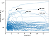 |
Fig. 4. Example of the mass growth history of all the sub-haloes that end up in the MW’s FoF group. The top curve corresponds to the main progenitor of the MW. This particular simulation (C10 S910 in the notation of W24) has both a GES and an LMC analogue, which are indicated with the large black circles. A video of this particular simulation is available online. |
We quantify the effect of having a GES-like merger or LMC-like merger on the growth times of the MW halo in Table 2. A GES-like merger biases towards an earlier z50 (MWs with a GES-like merger have  , while without a GES requirement we find
  ), which makes sense, given that our selection criteria require no major mergers (and thus no merger-associated growth) after the GES-like merger. Requiring an LMC-like object shifts z50 towards lower values only slightly: although one would expect to see the effect of the LMC in the growth history, in our definition, the LMC is required to be the most massive object at the present day. Because of that, any late major mergers with mass ratio μ > 0.2 are not considered in the subset, effectively disfavouring significant late growth. We find 12 simulations that have both a GES-like merger and an LMC analogue. In this case, as expected, z10 is biased early (and z90 in the opposite way), and also the scatter is somewhat reduced.
Mean and 16th and 84th percentiles of mass growth histories.
3.2. Understanding the growth in an LG environment
To further investigate how the MW and M31 have grown in our LG simulations, in the top panels of Fig. 5 we show the simulation presented in Fig. 4 and identify the positions at earlier times of the particles that end up in the MW and M31 FoF groups at the present day. In 65 out of 224 cases, the MW and M31 haloes end up in the same FoF group, and in these cases, the satellites are assigned to the closest halo. In this figure we have rotated and scaled the coordinate system such that the MW’s main progenitor is positioned at (x′,y′,z′) = (0, 0, 0), and M31’s main progenitor is at (1, 0, 0) at all times. This leaves one free angle (the rotation around the MW–M31 axis), which we set such that the z′-axis aligns as closely as possible with the north pole of the Local Sheet (at super-galactic coordinates (L, B) = (241.74° ,82.05° ), McCall 2014), which roughly aligns with the super-galactic north pole (the separation is 7.95°). As a result, the z′-axis maintains close alignment with the Local Sheet north pole. This is not exact because of M31’s slight elevation above the Local Sheet, but the misalignment is minor, averaging 23° at z = 7, and reducing to 12° at z = 0. The left column shows the distribution at redshift z ∼ 7, which reveals a few narrow filaments already forming with low z′ and a generally isotropic distribution around the two haloes. Then, at z ∼ 3.9, a large part of the MW’s material has collapsed into a sheet-like distribution, aligned with the z′ direction, with a filament forming along the MW-M31 axis. At z = 2, the collapse along the z′ direction is mostly complete, and further growth occurs mostly from within the sheet. By z = 1, this halo has accreted more than half of its material, and the distribution is again more axisymmetric around the MW-M31 axis.
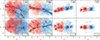 |
Fig. 5. Particles that end up in the MW sub-halo (in red) and in the M31 (in blue) by the present day, traced back to various redshifts for one of our realisations. Each column shows a different redshift. The coordinate system has been rotated and scaled such that the MW and M31 main progenitors are at (0,0,0) and (1,0,0), respectively, at all times (indicated with white dots). Top row: Approximately edge-on view of the Local Sheet. Bottom row: Face-on view. |
Although this is a single simulation, this behaviour is similar across all LG realisations, as depicted in Fig. 6. In this figure we stack all the MW and M31 progenitor particles of all simulations to get a map of the posterior mean behaviour of the positions of the progenitor particles over time (note that all simulations are samples from the LG posterior of W24, and hence stacking them gives the posterior mean field). At z = 7, the progenitor particle distribution is, on average, elongated along the z′-axis (which is roughly aligned with the super-galactic z-axis). Then up until z ∼ 2, it collapses along the z′-axis, becoming most compressed along this axis. After z = 2, the halo material starts to virialise and the distribution becomes roughly spherically symmetric by z = 1. The separatrix between the MW and M31 material is shown with black lines. It lies at x′ = 0.4 along the MW-M31 axis at z = 7.0; particles with x′< 0.4, are more likely to become part of the MW, and those with x′> 0.4 are more likely to become part of M31. Its location at x′ = 0.4 stays roughly constant throughout cosmic time, with some scatter ranging from 0.37 to 0.45. Interestingly, this range is expected from a simple computation of the location of the Lagrange point L1 in a system of two point masses (without rotation, as the tangential velocities are negligible) and with a mass ratio of 0.57 (which is the median value for our simulations).
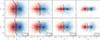 |
Fig. 6. Like Fig. 5 but now for the posterior mean of our simulations, a ‘stack’ of all LG re-simulations. The black lines are the isocontours at which a particle is equally likely to end up in the MW or M31. A video version of this figure is available online. |
Using Fig. 6 we can point out the effect that suppresses the MW’s mass growth at late times: due to the higher mass of M31, the particles that are right of the separatrix will go to M31 instead of the MW, and this especially suppresses late-time growth, when particles from larger initial distances dominate the mass growth. This is also seen in the un-normalised mass growth histories, shown in Appendix C, which at early times largely coincide and start to deviate at later times.
4. Discussion and conclusions
The MW haloes in our constrained LG simulations generally form earlier and grow more slowly at late times than their isolated counterparts. This is principally due to the presence of M31 (which is more massive by a factor of approximately 1.75 in the median) but may also be due in part to the quiet surrounding Hubble flow. The growth of both galaxy haloes is also quite anisotropic in our constrained simulations. Proto-halo material first collapses into a planar distribution, which is roughly aligned with the Local Sheet, and then, after z ∼ 2, starts to virialise, ending up in a significantly less flattened configuration by z ∼ 1.
Quantitatively, our MWs reach half their final mass at  , the M31s at
  , and the MW-mass and M31-mass isolated haloes from TNG50-DMO at
  . Requiring the LMM to be GES-like biases the MW to
  . The early- and late-time behaviour can be quantified as
  and (z90,MW, z90,M31)
  .
.
These values are not very different from those of Buch et al. (2024) for MW-like isolated haloes. They find a50 = 0.49 (z50 = 1.05) for a similar sample of MW-mass objects without the requirement of an LMC (in which case a50 = 0.57, z50 = 0.75), although on average, our MWs reach their half-mass slightly earlier. In the ELVIS suite of LG analogues, Garrison-Kimmel et al. (2019) and Santistevan et al. (2020) find that for isolated haloes z10 ∼ 3 and for LG-like hosts z10 ∼ 4, which is in agreement with our results. These authors argue that at later times, z ≲ 2, the mass growth histories of isolated and LG-like hosts are more similar, which might indicate that the initial overdensity associated with the LG in comparison to a random MW or M31 progenitor plays a role.
Similar findings are reported for the HESTIA simulations of LG-like pairs inside constrained simulations of the large-scale structure (with constraints on scales larger than ∼4 Mpc; Libeskind et al. 2020). In these simulations, on average z50 = 1.4, indicating that these haloes form roughly one billion years earlier than in unconstrained similarly massed MW or M31 analogues (whose z50 is ∼1.1). Note, however, that these authors make no distinction between MW and M31 haloes in their estimates of z50, so these numbers reflect the effect of a group environment and not differences between the two systems. In a sample of LGs extracted from CLUES (Carlesi et al. 2016), Carlesi et al. (2020) find that the median half-mass time of galaxy haloes in LGs in constrained realisations is also earlier than in LGs without constraints, although the difference is small, of the order of 0.5 Gyr both for the MWs and M31s. Carlesi et al. (2020) notice that their MWs reach their half-mass earlier than their M31s (by 0.25 Gyr) but attribute this difference to mass. We, on the other hand, find that our MWs also have a shorter average half-mass time than isolated MW-mass galaxies. The difference between MWs and M31s we find is also larger, ⟨t50,M31⟩ − ⟨t50,MW⟩ = 0.6 Gyr. This could plausibly be explained by the separation between our LG pairs, which is  , whereas Carlesi et al. (2020) allow for a much larger range of 0.5 − 1.9 Mpc. This may imply a larger separation between MW and M31 on average in their sample (see e.g. Table 7 of Carlesi et al. 2016), which would reduce the effect of M31 on the MW.
These findings may have implications for the formation of the Galactic disc, as explored by Semenov et al. (2024) using the TNG50 simulations. It appears that relatively few MW-mass disc galaxies in typical environments assembled a significant fraction of their mass within the first few billion years and formed a disc that has survived until the present day (fewer than 10%). Nevertheless, this seems to have happened in the real MW. However, we find that once the LG structure and its local environment are correctly reproduced, such behaviour is common. Increasing the chance of such an early assembly history requires (i) a quiet environment surrounding the LG and (ii) a relatively large mass ratio of M31 to the MW; both factors reduce the likelihood of significant late-time growth.
Possible improvements to the analysis presented here would include using a larger sample to increase the numerical precision of our estimates. This could also allow us to be stricter in selecting close analogues of the MW and M31, for example by identifying LMC-like objects that also reproduce the LMC’s present-day distance and approximate orbit. For a high-quality match, however, a preferable approach would be to add the LMC (or M33) as an extra constraint to the W24 methodology. Another possibility would be to constrain the spin orientation of the inner MW and M31 haloes to match the observed orientations of the two galaxies. A further obvious improvement would be to carry out hydrodynamical galaxy formation simulations, as they would allow us to follow the mass growth of all the different constituents of the galaxies, i.e. cold gas, hot gas, and stars, as well as the dark matter. We are currently working on such a suite of simulations and hope to report on them in future work.
Data availability
Movies associated to Figs. 4 and 6 are available at https://www.aanda.org
This selection was made from a homogeneous subsample of the chains, after excluding 15 cases (out of 239 total), where either the MW or M31 was part of a galaxy pair (defined as having a satellite with mass ratio > 0.3).
We ran the chains from W24 twice as long to increase the effective sample size. In Appendix B we discuss in more detail the degree to which the realisations can be considered to be (quasi-)independent.
Although this is relatively low given that first-order LPT was used, the differences in mass growth history compared to simulations started at z = 127 are negligible.
We also considered M100c, for which all results in this paper remain qualitatively unchanged. Generally, the effects reported in this paper and associated with the environment are enhanced for M100c as this encompasses mass in a more extended region.
In fact, if instead of the above selection we had simply required that the sub-halo be the central sub-halo of its FoF group, we would have found a very similar sample of 56 MW-mass and 56 M31-mass haloes.
This differs from the Neff = 27 reported in W24 due to a programming error in the effective sample size calculation in that paper. The results of W24 are unaffected, as all quoted uncertainties reflect the posterior widths, which are independent of the effective sample size. The corrected effective sample size of Neff = 20 inflates the predictive uncertainties on inferred quantities by 2.5%, compared to 1.7% with Neff = 27. This difference remains negligible.
Acknowledgments
This work has been financially supported by a Spinoza Prize from NWO to AH. EW thanks Dylan Nelson for providing access to the TNG simulations, Anna Genina and Victor Forouhar Moreno for helpful discussions, and Akshara for her moral support. We are grateful to the referee for a constructive report. The Gadget simulations were performed on the Freya cluster at the Max Planck Computing and Data Facility. The constrained simulations were enabled by resources provided by the Swedish National Infrastructure for Computing (SNIC) at the PDC Center for High Performance Computing, KTH Royal Institute of Technology, partially funded by the Swedish Research Council through grant agreement no. 2018-05973. JJ and GL acknowledge support from the Simons Foundation through the Simons Collaboration on “Learning the Universe”. This work was made possible by the research project grant “Understanding the Dynamic Universe”, funded by the Knut and Alice Wallenberg Foundation (Dnr KAW 2018.0067). Additionally, JJ acknowledges financial support from the Swedish Research Council (VR) through the project “Deciphering the Dynamics of Cosmic Structure” (2020-05143). GL acknowledges support from the CNRS-IEA “Manticore” project. This work is done within the Aquila Consortium (https://www.aquila-consortium.org/). Software: During this work, we have made use of various software packages. This includes BORG (Jasche & Wandelt 2013; Jasche & Lavaux 2019), GADGET-4 (Springel et al. 2021), JAX (Bradbury et al. 2018), NUMPYRO (Phan et al. 2019), XARRAY (Hoyer & Hamman 2017; Hoyer et al. 2023), NUMPY (Harris et al. 2020), SCIPY (Virtanen et al. 2020), MATPLOTLIB (Hunter 2007), H5PY (https://www.h5py.org/), ASTROPY (Astropy Collaboration 2018, 2022), JUG (Coelho 2017).
References
- Astropy Collaboration (Price-Whelan, A. M., et al.) 2018, AJ, 156, 123 [Google Scholar]
- Astropy Collaboration (Price-Whelan, A. M., et al.) 2022, ApJ, 935, 167 [NASA ADS] [CrossRef] [Google Scholar]
- Belokurov, V., Erkal, D., Evans, N. W., Koposov, S. E., & Deason, A. J. 2018, MNRAS, 478, 611 [Google Scholar]
- Boylan-Kolchin, M., Springel, V., White, S. D. M., Jenkins, A., & Lemson, G. 2009, MNRAS, 398, 1150 [Google Scholar]
- Boylan-Kolchin, M., Springel, V., White, S. D. M., & Jenkins, A. 2010, MNRAS, 406, 896 [Google Scholar]
- Boylan-Kolchin, M., Besla, G., & Hernquist, L. 2011, MNRAS, 414, 1560 [NASA ADS] [CrossRef] [Google Scholar]
- Boylan-Kolchin, M., Bullock, J. S., & Kaplinghat, M. 2012, MNRAS, 422, 1203 [NASA ADS] [CrossRef] [Google Scholar]
- Bradbury, J., Frostig, R., Hawkins, P., et al. 2018, JAX: Composable Transformations of Python+NumPy Programs [Google Scholar]
- Buch, D., Nadler, E. O., Wechsler, R. H., & Mao, Y.-Y. 2024, ApJ, 971, 79 [Google Scholar]
- Buck, T. 2020, MNRAS, 491, 5435 [NASA ADS] [CrossRef] [Google Scholar]
- Buck, T., Obreja, A., Ratcliffe, B., et al. 2023, MNRAS, 523, 1565 [CrossRef] [Google Scholar]
- Busha, M. T., Marshall, P. J., Wechsler, R. H., Klypin, A., & Primack, J. 2011, ApJ, 743, 40 [NASA ADS] [CrossRef] [Google Scholar]
- Carlesi, E., Sorce, J. G., Hoffman, Y., et al. 2016, MNRAS, 458, 900 [NASA ADS] [CrossRef] [Google Scholar]
- Carlesi, E., Hoffman, Y., Gottlöber, S., et al. 2020, MNRAS, 491, 1531 [Google Scholar]
- Ciucă, I., Kawata, D., Ting, Y.-S., et al. 2024, MNRAS, 528, L122 [Google Scholar]
- Coelho, L. P. 2017, J. Open Res. Software, 5, 1 [Google Scholar]
- Deason, A. J., & Belokurov, V. 2024, New Astron. Rev., 99, 101706 [CrossRef] [Google Scholar]
- D’Souza, R., & Bell, E. F. 2018, Nat. Astron., 2, 737 [Google Scholar]
- Evans, T. A., Fattahi, A., Deason, A. J., & Frenk, C. S. 2020, MNRAS, 497, 4311 [Google Scholar]
- Fattahi, A., Navarro, J. F., Sawala, T., et al. 2016, MNRAS, 457, 844 [NASA ADS] [CrossRef] [Google Scholar]
- Gaia Collaboration (Brown, A. G. A., et al.) 2018, A&A, 616, A1 [NASA ADS] [CrossRef] [EDP Sciences] [Google Scholar]
- Gaia Collaboration (Vallenari, A., et al.) 2023, A&A, 674, A1 [NASA ADS] [CrossRef] [EDP Sciences] [Google Scholar]
- Garrison-Kimmel, S., Wetzel, A., Hopkins, P. F., et al. 2019, MNRAS, 489, 4574 [Google Scholar]
- Hammer, F., Puech, M., Chemin, L., Flores, H., & Lehnert, M. D. 2007, ApJ, 662, 322 [NASA ADS] [CrossRef] [Google Scholar]
- Harris, C. R., Millman, K. J., van der Walt, S. J., et al. 2020, Nature, 585, 357 [NASA ADS] [CrossRef] [Google Scholar]
- Helmi, A. 2020, ARA&A, 58, 205 [Google Scholar]
- Helmi, A., Babusiaux, C., Koppelman, H. H., et al. 2018, Nature, 563, 85 [Google Scholar]
- Hoyer, S., & Hamman, J. 2017, J. Open Res. Software, 5, 1 [Google Scholar]
- Hoyer, S., Roos, M., Joseph, H., et al. 2023, https://doi.org/10.5281/zenodo.10023467 [Google Scholar]
- Hunter, J. D. 2007, Comput. Sci. Eng., 9, 90 [NASA ADS] [CrossRef] [Google Scholar]
- Jasche, J., & Lavaux, G. 2019, A&A, 625, A64 [NASA ADS] [CrossRef] [EDP Sciences] [Google Scholar]
- Jasche, J., & Wandelt, B. D. 2013, MNRAS, 432, 894 [Google Scholar]
- Libeskind, N. I., Carlesi, E., Grand, R. J. J., et al. 2020, MNRAS, 498, 2968 [NASA ADS] [CrossRef] [Google Scholar]
- Liu, L., Gerke, B. F., Wechsler, R. H., Behroozi, P. S., & Busha, M. T. 2011, ApJ, 733, 62 [Google Scholar]
- Majewski, S. R., Schiavon, R. P., Frinchaboy, P. M., et al. 2017, AJ, 154, 94 [NASA ADS] [CrossRef] [Google Scholar]
- Mao, Y.-Y., Geha, M., Wechsler, R. H., et al. 2024, ApJ, 976, 117 [NASA ADS] [CrossRef] [Google Scholar]
- McCall, M. L. 2014, MNRAS, 440, 405 [NASA ADS] [CrossRef] [Google Scholar]
- Naidu, R. P., Conroy, C., Bonaca, A., et al. 2020, ApJ, 901, 48 [Google Scholar]
- Nelson, D., Pillepich, A., Springel, V., et al. 2019a, MNRAS, 490, 3234 [Google Scholar]
- Nelson, D., Springel, V., Pillepich, A., et al. 2019b, Comput. Astrophys. Cosmol., 6, 2 [Google Scholar]
- Phan, D., Pradhan, N., & Jankowiak, M. 2019, ArXiv e-prints [arXiv:1912.11554] [Google Scholar]
- Pillepich, A., Nelson, D., Springel, V., et al. 2019, MNRAS, 490, 3196 [Google Scholar]
- Pillepich, A., Sotillo-Ramos, D., Ramesh, R., et al. 2024, MNRAS, 535, 1721 [NASA ADS] [CrossRef] [Google Scholar]
- Renaud, F., Agertz, O., Andersson, E. P., et al. 2021, MNRAS, 503, 5868 [NASA ADS] [CrossRef] [Google Scholar]
- Santistevan, I. B., Wetzel, A., El-Badry, K., et al. 2020, MNRAS, 497, 747 [Google Scholar]
- Santos-Santos, I. M. E., Fattahi, A., Sales, L. V., & Navarro, J. F. 2021, MNRAS, 504, 4551 [NASA ADS] [CrossRef] [Google Scholar]
- Sawala, T., Frenk, C. S., Fattahi, A., et al. 2016, MNRAS, 457, 1931 [Google Scholar]
- Schaye, J., Crain, R. A., Bower, R. G., et al. 2015, MNRAS, 446, 521 [Google Scholar]
- Semenov, V. A., Conroy, C., Smith, A., Puchwein, E., & Hernquist, L. 2024, ArXiv e-prints [arXiv:2409.18173] [Google Scholar]
- Sotillo-Ramos, D., Pillepich, A., Donnari, M., et al. 2022, MNRAS, 516, 5404 [NASA ADS] [CrossRef] [Google Scholar]
- Springel, V., Wang, J., Vogelsberger, M., et al. 2008, MNRAS, 391, 1685 [Google Scholar]
- Springel, V., Pakmor, R., Zier, O., & Reinecke, M. 2021, MNRAS, 506, 2871 [NASA ADS] [CrossRef] [Google Scholar]
- Stewart, K. R., Bullock, J. S., Wechsler, R. H., Maller, A. H., & Zentner, A. R. 2008, ApJ, 683, 597 [NASA ADS] [CrossRef] [Google Scholar]
- Toth, G., & Ostriker, J. P. 1992, ApJ, 389, 5 [NASA ADS] [CrossRef] [Google Scholar]
- Vasiliev, E. 2023, Galaxies, 11, 59 [NASA ADS] [CrossRef] [Google Scholar]
- Virtanen, P., Gommers, R., Oliphant, T. E., et al. 2020, Nat. Methods, 17, 261 [Google Scholar]
- Wempe, E., Lavaux, G., White, S. D. M., et al. 2024, A&A, 691, A348 [NASA ADS] [CrossRef] [EDP Sciences] [Google Scholar]
Appendix A: Up-sampling of initial condition fields
In W24 we utilised a zoom scheme that involved splitting the initial condition field into two parts, a field for the low-resolution large box, sLR, and a field for the high-resolution zoom region, sHR. The zoom region has a box size of 10 Mpc, with 64 elements on a side, giving sHR a mesh cell size of  . For our re-simulations, we used a grid twice as fine for the zoom region while leaving the outer region unchanged. Therefore, we up-sampled the sHR field, from its original 643 size to a 1283 grid, preserving all the Fourier modes of the original sHR field, and randomly generating the modes at frequencies larger than the Nyquist frequency (per axis) of sHR.
To accomplish this, we combined two fields: our original field sHR, which sets the larger-scale modes, and a randomly generated field (sss ∼ 𝒩(0,1)) that sets the smallest-scale Fourier modes. To ensure that the final field is real-valued, we used the Hartley transform, which guarantees a real-valued output for a real-valued input. The Hartley transform ( ) of a real field (s) was computed from the Fourier transform (
 ). We set our new field’s modes by taking
  modes at frequencies lower than the Nyquist frequency of sHR (the large scales) and from
  at higher frequencies (the small scales). At the Nyquist frequencies, the modes are split equally across the positive and negative Fourier modes in the new field, to ensure that, if sss = 0, the process corresponds to pure trigonometric interpolation. Hence, when one, two, or three indices are ±iNy, the contribution of
  is weighted by
  ,
,  , and
, and  , respectively. Since the variance of a mode X = a𝒩(0, 1)+b𝒩(0, 1) is given by σ2 = a2 + b2, to conserve unit variance at these modes, the coefficient b for the small-scale field
  was set to
  , resulting in
  ,
,  , and
, and  for the three cases, respectively. Summarising, the modes of the new
  field are:
![Mathematical equation: $$ \begin{aligned} \hat{\boldsymbol{s}}_{\text{ HR}}^{\text{ new}} = {\left\{ \begin{array}{ll} \hat{\boldsymbol{s}}_{\text{ HR}}&\quad {\text{ if} \text{ the} \text{ absolute} \text{ values} \text{ of} \text{ all} \text{ indices} \text{ are} \text{ less} \text{ than}} i_{\text{ Ny}},\\ [0.8em] \hat{\boldsymbol{s}}_{\text{ ss}}&\quad {\text{ if} \text{ the} \text{ absolute} \text{ value} \text{ of} \text{ any} \text{ index} \text{ exceeds}} i_{\text{ Ny}},\\ [0.0em] \frac{1}{2}\hat{\boldsymbol{s}}_{\text{ HR}} + \sqrt{\frac{3}{4}}\hat{\boldsymbol{s}}_\text{ss}&\quad {\text{ if} \text{ exactly} \text{ one} \text{ index} \text{ is}} \pm i_{\text{ Ny}},\\ [0em] \frac{1}{4}\hat{\boldsymbol{s}}_{\text{ HR}} + \sqrt{\frac{15}{16}}\hat{\boldsymbol{s}}_\text{ss}&\quad {\text{ if} \text{ exactly} \text{ two} \text{ indices} \text{ are}} \pm i_{\text{ Ny}}, \\ [0em] \frac{1}{8}\hat{\boldsymbol{s}}_{\text{ HR}} + \sqrt{\frac{63}{64}}\hat{\boldsymbol{s}}_\text{ss}&\quad {\text{ if} \text{ all} \text{ indices} \text{ are}} \pm i_{\text{ Ny}}, \end{array}\right.} \end{aligned} $$](/articles/aa/full_html/2025/09/aa53744-25/aa53744-25-eq52.gif)
where the indices range from −Nss/2 to Nss/2, iNy = NHR/2 is the Nyquist index of the  field, and the last three cases apply only if no index exceeds iNy in absolute value.
Appendix B: Auto-correlation analysis
In this work we used initial conditions inferred from Hamiltonian Monte Carlo chains with relatively long auto-correlation lengths. As a result, some quantities extracted from the simulations may exhibit auto-correlation, which would increase the numerical error in the posterior means reported in this paper. For independent samples of a quantity Q, the standard deviation of the mean is  . For correlated samples, this becomes
  , where Neff is the effective sample size. The effective sample size is calculated as
  , where ρ(d) is the auto-correlation function of Q at lag d.
In W24, the auto-correlation function of the initial condition fields, ρsss(d), was found to follow an exponential decay, ρ(d) = e−d/L, with auto-correlation length L. Fitting the model to the 12 Hamiltonian Monte Carlo chains resulted in an effective sample size of Neff = 20 for the initial condition field.6 For this study we ran the same 12 chains for longer; this produced an effective sample size of the initial condition field of Neff = 32. From these chains, we extracted 224 realisations.
It is important to note that for quantities sensitive to the behaviour on small scales (e.g. below 1 Mpc), the correlation lengths between samples will be smaller; hence, the 224 realisations could be seen in this context as (quasi-)independent. We explain below how to quantify the numerical uncertainties on the various quantities discussed in this paper taking into account the quasi-independence of our samples.
As an example, we determined the effective sample size of a50. We assumed an exponential auto-correlation function (Ae−d/Ls) and that auto-correlation lengths (Ls) on small scales are a factor f smaller than those for the initial conditions, i.e. L = f × Ls. To estimate Ls, we fitted the auto-correlation function using NumPyro. We assumed a50 follows a log-normal distribution, lna50 ∼ 𝒩(μ, σ2), with an exponentially declining auto-correlation function:
![Mathematical equation: $$ \begin{aligned} \rho _{a_{50}}(d) = \langle (a_{50}[i] - \mu )(a_{50}[i+d] - \mu )\rangle = A e^{-d/L_s}. \end{aligned} $$](/articles/aa/full_html/2025/09/aa53744-25/aa53744-25-eq57.gif) (B.1)
(B.1)
We find that f = 0.70 ± 0.17 and A = 0.41 ± 0.7, giving an effective sample size of Neff = 73 ± 13. The Monte Carlo standard error on a50 is 0.01 for both the MW and M31, and the earlier average assembly reported in Section 3.1 is significant at the 1.7% level.
For the a50 of the mass bound to the main sub-halo, the difference between MW and M31 is even more significant, at 0.4%. In this case, we removed the 65 cases in which the MW and M31 ended up in the same FoF group, to avoid potential biases due to the differing behaviour in the Subfind unbinding procedure in the same-FoF-group and different-FoF-group scenarios. Specifically, the Subfind unbinding procedure only considers particles within the same FoF group, meaning the tidal effect of M31 lowers the MW mass in the same-FoF-group case, but not in the different-FoF-group scenario.
Appendix C: Un-normalised mass growth histories
Instead of the normalised growth histories shown in Fig. 1, one can also consider the un-normalised growth histories, which are shown in Fig. C.1. Note that the MW and M31 have very similar mass assembly histories at early times, diverging only around redshift 4.
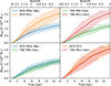 |
Fig. C.1. Top-left panel: Like Fig. 1 but un-normalised. Note that at early times, the MW and M31 had a very similar mass growth history, diverging from z ∼ 4. The larger scatter in the present-day M31 mass reflects the larger (observational) uncertainties on its mass from W24. Top-right panel: Same but for MW-mass and M31-mass galaxies from an unconstrained simulation. Bottom panels: Comparisons of the MWs and M31s from the constrained simulations with isolated MW- or M31-mass haloes. |
All Tables
Numerical parameters used in the LG Gadget-4 simulations presented in this paper.
All Figures
|
Fig. 1. Comparison of the mass growth histories of the MW and M31 galaxies from the constrained simulations of W24, compared to random MW- or M31-mass galaxies from TNG50-DMO. The central lines are the means, and shading indicates the 16–84 percentile regions. The un-normalised mass growth histories are shown in Appendix C. |
| In the text | |
|
Fig. 2. Distribution of the redshifts at which half the final mass was accumulated (z50) for the constrained MW and M31 haloes, compared to the random MW- or M31-mass haloes from TNG50-DMO. |
| In the text | |
|
Fig. 3. Merger-associated mass accretion rates as a function of infall time and mass ratio (μ). For each bin, the peak masses of the infalling objects are summed and normalised by the total merger-associated mass accretion for the respective halo (MW or M31). This normalised mass accretion rate (R) is then averaged over simulations, with the resulting values shown by the colours. Left panel: This quantity for the MW. Right panel: Difference between the MW and M31. The histograms at the bottom represent the same quantity but marginalised over mass ratio, showing the 1D distribution as a function of infall time. |
| In the text | |
|
Fig. 4. Example of the mass growth history of all the sub-haloes that end up in the MW’s FoF group. The top curve corresponds to the main progenitor of the MW. This particular simulation (C10 S910 in the notation of W24) has both a GES and an LMC analogue, which are indicated with the large black circles. A video of this particular simulation is available online. |
| In the text | |
|
Fig. 5. Particles that end up in the MW sub-halo (in red) and in the M31 (in blue) by the present day, traced back to various redshifts for one of our realisations. Each column shows a different redshift. The coordinate system has been rotated and scaled such that the MW and M31 main progenitors are at (0,0,0) and (1,0,0), respectively, at all times (indicated with white dots). Top row: Approximately edge-on view of the Local Sheet. Bottom row: Face-on view. |
| In the text | |
|
Fig. 6. Like Fig. 5 but now for the posterior mean of our simulations, a ‘stack’ of all LG re-simulations. The black lines are the isocontours at which a particle is equally likely to end up in the MW or M31. A video version of this figure is available online. |
| In the text | |
|
Fig. C.1. Top-left panel: Like Fig. 1 but un-normalised. Note that at early times, the MW and M31 had a very similar mass growth history, diverging from z ∼ 4. The larger scatter in the present-day M31 mass reflects the larger (observational) uncertainties on its mass from W24. Top-right panel: Same but for MW-mass and M31-mass galaxies from an unconstrained simulation. Bottom panels: Comparisons of the MWs and M31s from the constrained simulations with isolated MW- or M31-mass haloes. |
| In the text | |
Current usage metrics show cumulative count of Article Views (full-text article views including HTML views, PDF and ePub downloads, according to the available data) and Abstracts Views on Vision4Press platform.
Data correspond to usage on the plateform after 2015. The current usage metrics is available 48-96 hours after online publication and is updated daily on week days.
Initial download of the metrics may take a while.