| Issue |
A&A
Volume 701, September 2025
|
|
|---|---|---|
| Article Number | A122 | |
| Number of page(s) | 15 | |
| Section | Extragalactic astronomy | |
| DOI | https://doi.org/10.1051/0004-6361/202553760 | |
| Published online | 05 September 2025 | |
Little impact of mergers and galaxy morphology on the production and escape of ionizing photons in the early Universe
1
INAF – Osservatorio Astronomico di Roma, Via Frascati 33 00078 Monteporzio Catone, Italy
2
Institute of Science and Technology Austria (ISTA), Am Campus 1 A-3400, Klosterneuburg, Austria
3
Institute for Astronomy, University of Edinburgh, Royal Observatory, Edinburgh EH9 3HJ, UK
4
Center for Astrophysics, Harvard & Smithsonian, Cambridge, MA 02138, USA
5
Department of Physics and Astronomy, Williams College, Williamstown, MA 01267, USA
6
Instituto de Astrofísica de Andalucía (CSIC), Apartado 3004 18080 Granada, Spain
7
European Space Agency (ESA), European Space Astronomy Centre (ESAC), Camino Bajo del Castillo s/n 28692 Villanueva de la Cañada, Madrid, Spain
8
Department of Astronomy and Astrophysics, The Pennsylvania State University, University Park, PA 16802, USA
9
Institute for Computational and Data Sciences, The Pennsylvania State University, University Park, PA 16802, USA
10
Institute for Gravitation and the Cosmos, The Pennsylvania State University, University Park, PA 16802, USA
11
Centro de Astrobiología, Consejo Superior de Investigaciones Científicas, Madrid, Spain
12
Department of Physics, 196A Auditorium Road, Unit 3046, University of Connecticut, Storrs, CT 06269, USA
13
University of Massachusetts Amherst, 710 North Pleasant Street, Amherst, MA 01003-9305, USA
14
NSF’s National Optical-Infrared Astronomy Research Laboratory, 950 N. Cherry Ave., Tucson, AZ 85719, USA
15
University of Louisville, Department of Physics and Astronomy, 102 Natural Science Building, Louisville, KY 40292, USA
16
Department of Physics and Astronomy, Texas A&M University, College Station, TX 77843-4242, USA
17
George P. and Cynthia Woods Mitchell Institute for Fundamental Physics and Astronomy, Texas A&M University, College Station, TX, USA
18
Instituto de Astrofísica de Canarias, C/Vía Láctea s/n-La Laguna, Spain
19
Space Telescope Science Institute, 3700 San Martin Drive, Baltimore, MD 21218, USA
20
Laboratory for Multiwavelength Astrophysics, School of Physics and Astronomy, Rochester Institute of Technology, 84 Lomb Memorial Drive, Rochester, NY 14623, USA
21
National Astronomical Observatory of Japan, 2-21-1 Osawa, Mitaka, Tokyo 181-8588, Japan
22
Astronomy Centre, University of Sussex, Falmer, Brighton BN1 9QH, UK
23
Institute of Space Sciences and Astronomy, University of Malta, Msida MSD 2080, Malta
24
The University of Texas, Austin, TX, USA
⋆ Corresponding author: This email address is being protected from spambots. You need JavaScript enabled to view it.
Received:
15
January
2025
Accepted:
7
July
2025
Abstract
Compact, star-forming galaxies with high star formation rate surface densities (ΣSFR) are often efficient Lyman continuum (LyC) emitters at z ≤ 4.5, likely because intense stellar feedback creates low-density channels that allow photons to escape. Irregular or disturbed morphologies, such as those resulting from mergers, can also facilitate LyC escape by creating anisotropic gas distributions. We investigated the influence of galaxy morphology on LyC production and escape at redshifts 5 ≤ z ≤ 7 using observations from various James Webb Space Telescope (JWST) surveys. Our sample consists of 436 sources, which are predominantly low-mass (∼108.15 M⊙), star-forming galaxies with ionizing photon efficiency (ξion) values consistent with canonical expectations. Since direct measurements of fesc are not possible during the Epoch of Reionization (EoR), we predicted fesc for high-redshift galaxies by applying survival analysis to a subsample of LyC emitters from the Low-Redshift Lyman Continuum Survey (LzLCS), selected to be direct analogs of reionization-era galaxies. We find that these galaxies exhibit, on average, modest predicted escape fractions (∼0.04). In addition, we evaluated the correlation between morphological features and LyC emission. Our findings indicate that neither ξion nor the predicted fesc values show a significant correlation with the presence of merger signatures. This suggests that in low-mass galaxies at z ≥ 5, strong morphological disturbances are not the primary mechanism driving LyC emission and leakage. Instead, compactness and star formation activity likely play a more pivotal role in regulating LyC escape.
Key words: galaxies: evolution / galaxies: formation / galaxies: high-redshift / galaxies: interactions
© The Authors 2025
 Open Access article, published by EDP Sciences, under the terms of the Creative Commons Attribution License (https://creativecommons.org/licenses/by/4.0), which permits unrestricted use, distribution, and reproduction in any medium, provided the original work is properly cited.
This article is published in open access under the Subscribe to Open model. This email address is being protected from spambots. You need JavaScript enabled to view it. to support open access publication.
1. Introduction
The Epoch of Reionization (EoR) marks a crucial phase in the Universe’s history, beginning with the formation of the first stars at z ∼ 20 − 30 (e.g., Barkana & Loeb 2001) and concluding around z ∼ 5.5, when reionization was complete (e.g., Bosman et al. 2022). During this period, the first luminous sources, such as active galactic nuclei (AGNs) and massive stars in the early galaxies, emitted ionizing photons that reionized the neutral hydrogen in the intergalactic medium (IGM). While AGNs have been proposed as potential contributors to reionization (e.g., Madau & Haardt 2015; Finkelstein et al. 2019; Madau et al. 2024; Dayal et al. 2025), the consensus is that young, hot stars in star-forming galaxies were the primary drivers Robertson & Schneider 2013; Atek et al. 2024; Asthana et al. 2024. These stars produced ultraviolet (UV) radiation, specifically in the Lyman continuum (LyC, λ < 912 Å), which ionized surrounding hydrogen and played a key role in transforming the early Universe.
The ability of these galaxies to provide the necessary number of ionizing photons to reionize the Universe depends on the escape fraction (fesc) of the LyC photons, the percentage of LyC photons that successfully escape the galaxies’ interstellar medium (ISM) and circumgalactic medium (CGM) to reach the IGM. An average fesc of around 0.1 across all galaxies is estimated to be necessary to match the reionization history, as predicted by independent constraints including cosmic microwave background (CMB) data Planck Collaboration VI 2020 and high-redshift galaxy luminosity functions (e.g., Robertson et al. 2015; Yung et al. 2020a,b; Finkelstein et al. 2019). However, directly measuring fesc at z ≥ 4.5, where reionization occurred, is impossible due to the increasing IGM opacity at that epoch Inoue et al. 2014.
One avenue to address this challenge is to study low-redshift galaxies with measurable LyC leakage, to search for properties that are analogous to those of galaxies in the EoR. These lower-redshift galaxies, known as Lyman continuum emitters (LCEs), allow astronomers to measure LyC escape fractions and explore the conditions in the ISM that facilitate LyC photon escape Izotov et al. 2016a, 2020; Verhamme et al. 2017; Schaerer et al. 2022; Saxena et al. 2022; Flury et al. 2022a,b; Chisholm et al. 2022; Saldana-Lopez et al. 2022. These measurements are then used to infer the average fesc of cosmic reionizers (e.g., Jung et al. 2024a; Mascia et al. 2023, 2024; Roy et al. 2023; Saxena et al. 2024; Li et al. 2023), consistently finding an average fesc lower than 0.1.
Among the many programs analyzing the properties of low-redshift LyC leakers, the most comprehensive is the Low-Redshift Lyman Continuum Survey (LzLCS, GO 15626, PI Jaskot) Flury et al. 2022a,b; Saldana-Lopez et al. 2022. The LzLCS sample was supplemented with archival COS observations from Izotov et al. 2016b, 2018a,b, 2021; Wang et al. 2019. The combined dataset, referred to as the LzLCS+ sample, includes 88 low-redshift galaxies with either detections or stringent limits on LyC emission. The survey tested various indirect diagnostics to understand their correlation with LyC emission and found that indicators based on Lyα emission are particularly effective: LyC emitters tend to have a high Lyα escape fraction and a small velocity peak separation. Additionally, properties such as high [O III]λλ4960, 5008/[O II] λ3727 (O32) flux ratio, high specific star formation rate surface density (ΣsSFR), and a blue UV slope β Chisholm et al. 2022 also correlate with a high LyC escape Flury et al. 2022a.
Although many properties correlate with fesc, such relations are extremely scattered; for this reason, several authors have refined methods to predict LyC emission using a combination properties, called multivariate diagnostics. Initial studies Mascia et al. 2023, 2024; Lin et al. 2024 employ traditional regression methods. However, these models often struggle with censored data, datasets that include upper limits rather than exact measurements. Furthermore, these methods assume a linear relationship between the variables and fesc, a condition that may not always be met. Recently, Jaskot et al. 2024a,b have proposed survival analysis techniques, which are better suited to the nature of the LzLC+ dataset, with its broad range of fesc values and numerous upper limits. Ignoring these upper limits could lead to biased predictions and inaccurate insights into what differentiates galaxies that emit LyC radiation from those that do not (e.g., Isobe et al. 1986). One of the most promising models is the TopThree Jaskot et al. 2024b, which incorporates three key predictors: the star formation rate surface density (ΣSFR = SFR/(2πre2), where re is the UV half-light radius), the O32 ratio, and the UV slope (β). It has been noted that a high ΣSFR correlates with efficient LyC photon escape (e.g., Heckman et al. 2001; Naidu et al. 2020; Flury et al. 2022a), particularly in compact galaxies where intense star formation feedback creates low-density channels in the ISM. These channels facilitate LyC photon escape, resulting in a higher fesc. For instance, J1316+2614, a galaxy at z = 3.613, is noted as one of the brightest LyC emitters known, with an escape fraction of approximately 0.9. This galaxy’s compact morphology, characterized by a half-light radius of re ∼ 0.22 kpc and an extremely high log10ΣSFR ≈ 3.47M⊙yr−1kpc2, suggests that intense star formation efficiency plays a critical role in driving LyC escape Marques-Chaves et al. 2022, 2024. This is a prediction from multiple generations of models (e.g., Wise & Cen 2009; Bhagwat et al. 2024).
Although compactness and high ΣSFR are common in many LCEs, they are not universally present. Some LCEs exhibit more extended or irregular structures, likely shaped by processes such as galaxy mergers or interactions (e.g., Bergvall et al. 2013). A notable merging system with detected LyC flux is Haro 11 at z = 0.02, which, however, has only a modest escape fraction. Another source that shows both LyC emission and evidence of mergers is z19863 at z = 3.088 (e.g., Rivera-Thorsen et al. 2017; Gupta et al. 2024). Finally, Maulick et al. 2024 report LyC emission from a merging system at z = 1.097. Indeed, mergers can lead to inhomogeneous gas distributions, where tidal interactions strip gas and stars, resulting in complex morphologies Toomre & Toomre 1972; Cox et al. 2008; Pearson et al. 2019; Spilker et al. 2022. These irregularities can result in anisotropic gas distributions, with pockets of optically thin neutral hydrogen allowing LyC photons to escape. In Haro 11, deep 21 cm observations have revealed reduced gas density pockets, likely due to recent merger activity, facilitating LyC photon escape Le Reste et al. 2024. Further supporting the link between mergers and LyC escape observed by Yuan et al. 2024, are the spatial offsets between the ionizing and non-ionizing radiation observed in several sources such as the famous Sunburst arc (z = 2.4, Rivera-Thorsen et al. 2017, 2019; Mainali et al. 2022) where LyC emission originates from a leaking star-forming knot distinct from the rest of its host galaxy. Other examples are reported by Yuan et al. 2024 and Ji et al. 2020.
The diversity in LCE morphologies highlights the importance of galaxy structure and gas distribution in determining LyC escape. In particular, the anisotropic coverage of neutral gas, rather than relying solely on simplified one-dimensional indicators such as the O32 ratio – which can also be influenced by variations in metallicity and ionization parameters (e.g., Bassett et al. 2019; Katz et al. 2020) – may play a crucial role in regulating the escape of LyC photons. Studies have shown that LCEs with disturbed morphologies often exhibit weaker correlations between the O32 ratio and fesc, suggesting that gas geometry and distribution are critical factors Bassett et al. 2019.
With the advent of the James Webb Space Telescope (JWST, Gardner et al. 2023), we now have the capability to probe indirect indicators at unprecedented depths, enabling the measurement of fesc for a large and diverse sample of galaxies during the EoR. Thanks to JWST’s Near-Infrared Camera (NIRCam), we are also refining our understanding of the morphology of these early sources (e.g., Treu et al. 2023; Dalmasso et al. 2024). Current findings indicate that signatures of mergers and interactions are detected in approximately 30% of the galaxies studied at z ≥ 5.5. Recent work by Calabrò et al. 2024 shows that, in the GLASS-JWST and the Cosmic Evolution Early Release Science (CEERS) spectroscopic surveys, ΣSFR at z ≥ 7 correlates with the O32 ratio and therefore with indirect estimates of the LyC escape fraction.
Recent findings by Simmonds et al. 2024 demonstrate that galaxies during the EoR that are characterized by low stellar masses and bursty star formation histories (SFHs) exhibit the highest values of ξion, driven by the dominance of younger stellar populations. This bursty star formation scenario is consistent with recent results from stacking analyses of the LzLCS sample Flury et al. 2025, which suggest that such SFHs provide the optimal feedback and geometric conditions necessary for efficient LyC escape.
The aim of this study is to systematically explore the impact of galaxy morphology, star formation activity, and gas distribution on the physical processes driving LyC production and escape in galaxies during the EoR.
The paper is structured as follows. In Sect. 2, we describe the sample selection. In Sect. 3, we present the methodology for line measurements, the SED fitting process, the general properties of the sources, and the mergers identification criteria. In Sect. 4 we introduce a revised survival analysis to predict the fesc for our sample. In Sect. 5, we report the predicted fesc, analyze the correlation of the presence of merger signatures with fesc and ξion, and interpret our results. In Sect. 6, we summarize our key findings. Throughout this work, we assume a flat Λ cold dark matter cosmology with H0 = 67.7 km s−1 Mpc−1 and Ωm = 0.307 Planck Collaboration VI 2020 and the Chabrier 2003 initial mass function. All magnitudes are expressed in the AB system Oke & Gunn 1983.
2. Data
2.1. EIGER data
We selected 133 sources from the Emission-line Galaxies and Intergalactic Gas in the Epoch of Reionization (EIGER) survey (GTO 1243, PI: Lilly, Kashino et al. 2023). This study leverages the first deep 3.5 μm JWST/NIRCam Wide Field Slitless Spectroscopy (WFSS) observations from the EIGER program, focusing on spectroscopically confirmed [O III] emitters at redshifts z = 5.33 − 6.93. These sources are located in the field of the bright quasar SDSS J010013.02+280225.8, though the majority are not directly associated with the quasar. A comprehensive list of identified sources and detection methods is available in Kashino et al. 2023; Matthee et al. 2023. The dataset is further complemented by EIGER NIRCam imaging in three broadband filters (F115W, F200W, and F356W). Further details on the imaging data reduction and analysis are presented in Kashino et al. 2023 and Matthee et al. 2023.
Our focus is on sources in the redshift range 5 ≤ z ≤ 7, which were identified using NIRCam WFSS in the F356W filter, where the [O III] and Hβ emission lines are detectable. For point sources, the spectral resolution is approximately R ∼ 1500 at 3.5 μm, with a dispersion of about 1 nm per pixel.
Emission lines were detected with a minimum signal-to-noise ratio (S/N) of 3, with a 3σ limiting sensitivity varying across the field and with wavelength (by a factor of approximately two), reaching 0.6 × 10⁻¹⁸ erg s−1 cm−2 at 3.8 μm. After visual inspection and parameter refinement, 133 resolved [O III]-emitting components within the redshift range z = 5.33 − 6.93 were identified, each with at least two detected emission lines at S/N > 3. The typical S/N for the [O III]λ5008 line is 14 (ranging from 6 to 70), while Hβ is detected with S/N > 3 in 68 objects, with 31 of these reaching S/N > 5. Only three of the 133 objects were primarily identified via Hβ, where [O III]λ4960 had S/N < 3.
2.2. CEERS and Director’s Discretionary Program (DD-2750) data
We selected sources from CEERS (ERS 1345, PI: Finkelstein) in the Extended Groth Strip (EGS) field of the Cosmic Assembly Near-infrared Deep Extragalactic Legacy Survey (CANDELS, Grogin et al. 2011; Koekemoer et al. 2011). In particular, we selected all sources with 5 ≤ zspec ≤ 7 from Napolitano et al. 2024; Mascia et al. 2024 that have a NIRSpec spectrum obtained either with the three medium-resolution (R ≈ 1000) grating spectral configurations (G140M/F100LP, G235M/F170LP and G395M/F290LP), which together cover wavelengths between 0.7–5.1 μm, or with the PRISM/CLEAR configuration, which provides continuous wavelength coverage of 0.6–5.3 μm with spectral resolution ranging from R ∼ 30 to 300. The total number of sources is 28.
All sources have available photometry with JWST/NIRCam filters (F115W, F150W, F200W, F277W, F356W, F444W, and F410M), as well as HST/ACS filters (F606W, F814W) and HST/WFC3 filters (F105W, F125W, F140W, and F160W) Bagley et al. 2023; Finkelstein et al. 2022a,b. To maintain consistency with the EIGER sample, we applied a cut in the F115W magnitude at 28.5 AB during the selection process.
In addition, we also considered sources from a DDT program in the same field (DDT 2750, PI: Arrabal Haro). These sources were observed using the PRISM/CLEAR configuration and possess the same photometric information as the sources from the CEERS sample. We determined the redshifts of the galaxies by analyzing the 1D spectrum with the redshift-fitting module of MSAEXP1. This module assesses the goodness of fit across a redshift range of 0 to 15, employing a series of EAzY Brammer 2021 galaxy and line templates at the nominal NIRSpec/PRISM resolution. Each galaxy was fitted individually, and the resulting solutions were visually inspected. Similar to the CEERS sources, during the selection phase we implemented a cutoff for the F115W magnitude at 28.5 AB. In total we added 15 sources from this sample, in the redshift range of interest.
2.3. JADES data
We selected sources from the JWST Advanced Deep Extragalactic Survey (JADES, GTO 1180, GTO 1210, GTO 1286 and GO 3215, Eisenstein et al. 2023) in the Great Observatories Origins Deep Survey (GOODS, Giavalisco et al. 2004) South and in North fields. All sources have available photometry with JWST/NIRCam filters (F115W, F150W, F200W, F277W, F356W, F444W, and F410M), as well as HST/ACS filters (F606W, F814W) and HST/WFC3 filters (F105W, F125W, F140W, and F160W) Merlin et al. 2024.
We restricted the sample to sources with spectroscopic redshifts 5 ≤ z ≤ 7 from Data Release 3 D’Eugenio et al. 2025. The sources have NIRSpec spectra obtained either with the three medium-resolution grating spectral configurations (G140M/F100LP, G235M/F170LP, and G395M/F290LP), or with the PRISM/CLEAR configuration. We included all sources within the specified redshift range flagged as “A”, “B”, or “C”, indicating emission lines detected in the grism or prism configuration, respectively, or secure redshifts visually identified from spectral breaks and/or low S/N emission lines. The final number of sources selected was 152 in the GOODS-S field and 108 in the GOODS-N field.
The list of datasets and their targeted fields is presented in Table 1. When combined with the other samples, our final dataset comprises a total of 436 sources observed during the EoR. Fig. 1 illustrates the distribution of our total sample across the z − M1500 plane. All M1500 values were computed using Prospector (see Sect. 3).
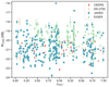 |
Fig. 1. M1500 − z distribution for the 436 sources with 5 ≤ zspec ≤ 7 analyzed in this work. |
Summary of JWST datasets and number of confirmed sources with redshifts 5 ≤ z ≤ 7 included in this study.
3. Methods
3.1. SED fitting
The physical properties of the EIGER sources, presented in Matthee et al. 2023, have been estimated using the Prospector code Johnson et al. 2021. To ensure consistency in the derivation of physical properties across our entire sample, we used the same code, incorporating a nebular treatment based on Cloudy version 13.03 Ferland et al. 1998; Byler et al. 2017, to fit the spectral energy distributions (SEDs) of sources from the other public programs. This approach allowed us to uniformly fit the available multiband JWST and HST photometry across the dataset.
Consistent with the methodology outlined by Matthee et al. 2023, the free parameters in our modeling included the total formed stellar mass, stellar metallicity, star formation history, dust attenuation, gas-phase metallicity, and ionization parameter. The redshift was fixed based on the spectroscopic measurement, and we assumed a Chabrier 2003 initial mass function along with MIST isochrones Dotter 2016; Choi et al. 2016. The star formation history followed a delayed-τ model, ψ(t) = ψ0te−t/τT. Both stellar and nebular emissions were attenuated by dust using a simple screen model with a Calzetti et al. 2000 law.
We employed uniform and broad priors in our model: the stellar mass was allowed to vary between 106 and 1011 M⊙, stellar metallicity between [Z/H]= − 2.0 and +0.2, dust optical depth τ between 0 and 2, stellar age between 1 Myr and the age of the Universe at the galaxy’s redshift, and the star formation timescale τT between 100 Myr and 20 Gyr. Gas-phase metallicity was modeled in the range 12 + log(O/H) = 6.7 to 9.2, while the ionization parameter U spanned from −3 to +1 on a logarithmic scale, allowing for higher values to provide greater flexibility in the fits.
The distributions of the main properties of the sources in this sample are presented in Fig. 2. The resulting SED fits suggest that dust attenuation in our galaxies is minimal, with a median E(B − V) = 0.07. The galaxies’ observed UV magnitudes range from MUV = −16.1 to −24.6 (with a typical MUV = −20.46), and their stellar masses span three orders of magnitude, from log10(M/M⊙) = 6.76 to 10.9, with a median mass of 108.15 M⊙.
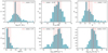 |
Fig. 2. Stellar mass, log10(M⋆); UV magnitude, M1500; β slope; E(B–V); and log10(sSFR) for 436 sources in our sample, derived using Prospector. The ionizing photon production efficiency, log10ξion, was calculated for all sources with detectable Hα or Hβ using the relations proposed by Leitherer & Heckman 1995; Schaerer et al. 2016. The figure shows the median values along with their standard deviations (16th and 84th percentiles) for each distribution. |
3.2. Line measurements and ξion estimation
The catalog of emission lines that were detected in the EIGER sample is available Kashino et al. 2023, providing fluxes and equivalent widths (EW) for the Hβ and [O III] doublet lines.
For the remaining samples, we measured emission lines using LIME2 Fernández et al. 2024, a versatile tool for analyzing medium-resolution and PRISM/CLEAR 1D spectra. The tool requires the source’s 1D spectrum, spectroscopic redshift, and a predefined list of lines to fit. Our analysis focused on key emission lines, including [O II], Hβ, [O III], and Hα. We used LIME to estimate the continuum and compute direct integration and Gaussian fluxes for lines with a S/N above 3, as well as their EWs.
Before any quantitative analysis, we corrected the line fluxes for dust reddening. Since Hα is not observed for most sources, we used stellar E(B-V) values derived from SED fitting to calculate the dust attenuation for each emission line, applying the Calzetti et al. 2000 extinction law. The total attenuation in magnitudes was given by AV = 0.44 × E(B-V) × κ, where κ is the wavelength-dependent attenuation coefficient for each line. The corrected fluxes were obtained by multiplying the observed fluxes by 10AV, with κHβ = 4.60, ![Mathematical equation: $ \kappa_\mathrm{[O{\small { {\text{ III}}}}]} = 4.46 $](/articles/aa/full_html/2025/09/aa53760-25/aa53760-25-eq1.gif) , and
, and ![Mathematical equation: $ \kappa_\mathrm{[O{\small { {\text{ II}}}}]} = 5.86 $](/articles/aa/full_html/2025/09/aa53760-25/aa53760-25-eq2.gif) Calzetti et al. 1997. We then computed O32 line ratios and rest-frame EWs for the [O III] doublet and/or Hβ.
Calzetti et al. 1997. We then computed O32 line ratios and rest-frame EWs for the [O III] doublet and/or Hβ.
Following Leitherer & Heckman 1995 and Schaerer et al. 2016, we inferred log ξion– under the assumption of zero LyC escape – from the dust-corrected Hα or Hβ luminosity, as these lines are clearly detected in 413 out of 436 sources (95% of the sample). The distribution of log ξion is shown in Fig. 2, with a median log ξion of 25.21.
Fig. 3 presents ξion as a function of MUV. We note that some sources exhibit extremely high log(ξion) values (> 27). Although these tend to be among the brighter objects, we cannot exclude that they are affected by measurement uncertainties or, in rare cases, by AGN contamination. However, due to the limited spectral coverage of our dataset–particularly for the EIGER subsample, where only [O III] and Hβ are available – we are currently unable to robustly identify or exclude AGN using standard diagnostics. We observe that ξion increases with MUV, consistent with the predictions at z ∼ 6 from Simmonds et al. 2024; Prieto-Lyon et al. 2023; Llerena et al. 2025. In our sample, fainter galaxies tend to have higher ξion values compared to brighter galaxies, although there is considerable scatter. This finding is in contrast to recent results by Pahl et al. 2025, which suggest that fainter galaxies are less efficient at producing ionizing photons than their brighter counterparts.
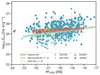 |
Fig. 3. Relation between log ξion and MUV. Each data point corresponds to an individual galaxy in our sample, with different symbols representing the various surveys. We include the curves from Simmonds et al. 2024; Pahl et al. 2025, as well as the relation from Llerena et al. 2025 at z ∼ 6. |
3.3. Mergers identification
In this study, we aim to determine whether galaxy mergers create channels that facilitate the production and escape of LyC photons during reionization. To investigate this, we analyzed NIRCam F115W images, available for all the surveys utilized in this work. These images trace the rest-frame UV at λmean ∼ 1916 Å for galaxies at z = 5 and λmean ∼ 1438 Å for galaxies at z = 7, thus providing a direct view of the ionizing stellar populations most relevant for LyC escape. While rest-optical imaging (e.g., F356W) traces the overall stellar distribution, we focused on the ionizing sources and their immediate environment, which are best captured in the UV. Furthermore, the F356W filter has lower spatial resolution and, depending on the redshift, can be significantly affected by strong nebular emission lines such as [O III] and Hβ, complicating morphological interpretation. Previous studies (e.g., Pawlik et al. 2016; Treu et al. 2023) show that merger signatures and clumpy star formation can be effectively identified in rest-frame UV images, supporting the use of this approach.
Following Treu et al. 2023, we created a segmentation map for each object to reduce noise and enhance low surface-brightness regions, which is particularly useful for galaxies with low S/N Pawlik et al. 2016. We applied a 6 × 6 uniform filter to the images and used the photutils package to generate the map, requiring at least five connected pixels with flux 2σ above the background. The binary detection mask (MD) is defined as the segmentation area corresponding to the target, excluding neighbors. From the MD, we derived the galaxy radius Rmax, given by the maximum pixel distance from the centroid (the brightest pixel in MD), which is more effective than the Petrosian radius for disturbed or low S/N morphologies Pawlik et al. 2016. We set a lower limit of 0.025″for spatial resolution; structures below this scale are considered unresolved.
We also measured a set of morphological parameters, including the Gini coefficient (G, Abraham et al. 2003), which quantifies the distribution of light in a galaxy and indicates howconcentrated or dispersed the light is; the second-order moment of brightness (M20, Lotz et al. 2004), which measures the spatial concentration of the brightest 20% of a galaxy’s light; and asymmetry (A, Abraham et al. 1996; Conselice et al. 2000), which assesses how the light distribution of a galaxy deviates from a perfectly symmetric shape. We successfully performed these measurements for 420 of the 436 sources (96% of the sample).
To identify mergers during the EoR, we applied two commonly used criteria from Conselice et al. 2003 and Lotz et al. 2008:
 (1)
(1)
 (2)
(2)
These criteria, initially developed for galaxies at z ≲ 1.2 Conselice et al. 2009, have been shown to work well at higher redshifts (e.g., Conselice & Arnold 2009; Treu et al. 2023; Vulcani et al. 2023; Dalmasso et al. 2024; Costantin et al. 2025). It is worth noting that these criteria are effective for identifying galaxies in the early stages of a merger but might be less suited to detect low surface-brightness features associated with post-merger stages Pawlik et al. 2016. It is not clear whether the creation of low-density channels in the ISM is associated with specific phases of the mergers; it might well be that such channels do not form in the early stages. This will discussed in more detail in the results section.
In accordance with Dalmasso et al. 2024, we defined the Silver sample as galaxies satisfying the Gini-M20 criterion (Eq. (1)), and the Gold sample as the subset of galaxies that also meet the asymmetry criterion (Eq. (2)). The Gold sample identifies mergers with more pronounced asymmetry, indicating more disruptive events, while the Silver sample captures mergers based primarily on light concentration. The results of this classification are illustrated in Fig. 4, with the two dashed lines indicating the threshold values calculated from Eqs. (1) and (2). A visual comparison between merger and non-merger candidates in our sample is provided in Fig. 5, where the associated f(G, M20) and A are also listed for reference. To ensure the accuracy of the classifications, we conducted a thorough visual inspection of all sources in both the Gold and Silver samples, which revealed no ambiguities.
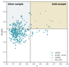 |
Fig. 4. Visual representation of our classification results in the A vs f(G, M20) diagram. Symbols are the same as in Fig. 3. The two dashed lines indicate the threshold values determined from Eqs. (1) and (2). |
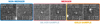 |
Fig. 5. Non-merger and merger candidates from the various surveys considered in this study, separated into Silver and Gold samples. Each row shows two representative sources for each category: non-merging systems; Silver sample mergers (selected based on the f(G, M20) criterion, Eq. (1)); and Gold sample mergers (satisfying both f(G, M20) and A criteria, Eqs. (1) and (2)). The cutouts, in the F115W filter, show the rest-frame UV at the redshift of each galaxy. The source ID, redshift, asymmetry (A), and Gini-M20 (f(G, M20)) values are provided for each stamp. |
The distribution of merger and non-merger signatures in our sample offers important insights into the nature of galaxies during the EoR. Quantitatively, only 13 of the 436 galaxies are part of the Gold sample (merger fraction fm = 0.03 ± 0.01), and 78 belong to the Silver sample (merger fraction fm = 0.17 ± 0.01). Notably, there are also 18 galaxies that exhibit highly asymmetric shapes, but are not selected as mergers. The vast majority – 311 galaxies – are compact systems. This distribution indicates that during the EoR, galaxies tend to be more compact rather than exhibiting major morphological disturbances.
Our findings are consistent with previous studies. For instance, Dalmasso et al. 2024 report a merger fraction for sources brighter than MUV = −20.1 for the Gold sample at z ∼ 6 of fm = 0.06 ± 0.03 and for the Silver sample of fm = 0.22 ± 0.04. These values were derived using high-resolution NIRCam JWST data in the low-to-moderate magnification (μ < 2) regions of the Abell 2744 cluster field. Additionally, their analysis reveals no significant differences in specific star formation rates between merger and non-merger signatures, reinforcing the notion that interactions may not play a major role in regulating star formation during this period. While our morphological approach is supported by both high-redshift JWST applications and low-redshift validations, we caution that alternative classifications may yield different outcomes. This underscores the need for a more systematic comparison, particularly with the LzLCS+ sample, in future studies.
4. A revised model to infer fesc using low-redshift analogs
4.1. Identifying LzLCS+ analogs of EoR sources
The LyC emitters from the LzLCS+ survey exhibit a wide range of physical properties, making them a diverse sample to study LyC escape Flury et al. 2022b. Their stellar masses range from approximately 107.2 M⊙ to 109.3 M⊙, and their MUV range from −21.3 to −18.3. The sample also exhibits considerable variability in dust content, reflected by β slopes ranging from −2.7 to −1.6 and reddening values, E(B-V), between 0.013 and 0.206. Because the LzLCS+ galaxies were selected to encompass diverse properties and test fesc diagnostics, they span a much wider (and in some cases different) range of properties than those observed during the EoR. Therefore, only a fraction of these can be considered true analogs of the sources currently detected by JWST in that era.
To account for these differences, we refined our predictions for fesc during reionization by comparing our sample of galaxies at 5 ≤ z ≤ 7 with the LzLCS+ sample, aiming to calibrate the low-redshift models using only true analogs of EoR galaxies. Fig. 6 presents the comparison between various properties of the galaxies, including β slope versus stellar mass, β versus MUV, and β versus dust reddening E(B-V). The gray-shaded area represents the density distribution of the sources in our EoR sample, with the contours in each panel indicating the 99% interval of the distributions, while individual points correspond to the LzLCS+ sources Based on the four properties shown in the figure, we find that only 51 galaxies in the LzLCS+ sample match the properties of EoR sources, as they consistently fall within the 99% distribution in each panel. Hereafter, we refer to this subsample as “analogs”. The mean properties indicate that the analogs are dust-poor (E(B-V) = 0.1), have a blue spectral slope (β = −2.1), a high O32 (∼9), a low stellar mass (log M⋆ = 8.6 M⊙), a MUV of approximately −19.65, and are compact in the UV (re ∼ 0.559 kpc). Additionally, the plots include known LyC leakers at z ∼ 3 from the literature (e.g., Vanzella et al. 2012, 2015, 2016; Vanzella et al. 2018; de Barros et al. 2016; Fletcher et al. 2019; Yuan et al. 2021; Marques-Chaves et al. 2022; Kerutt et al. 2024; Jung et al. 2024b), highlighting that even at this redshift, these galaxies exhibit a wide range of properties, not all of which make them analogs of EoR.
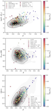 |
Fig. 6. Comparison of galaxy properties between z ∼ 0.3 LyC emitters from the LzLCS+ Flury et al. 2022b and high-redshift sources, shown as a density plot. Panels show log M⋆ vs. β slope (top), MUV vs. β (middle), and E(B-V) vs. β (bottom). Of the 88 LyC emitters, 51 galaxies are identified as analogs to high-redshift sources, falling within the 99% confidence interval in all panels. Known LyC leakers at z ∼ 3 are also included from the literature: Ion1 Vanzella et al. 2012, Ion2 Vanzella et al. 2015, 2016; de Barros et al. 2016, Ion3 Vanzella et al. 2018, J1316+2614 Marques-Chaves et al. 2022, CDFS-6664 Yuan et al. 2021, LACES Fletcher et al. 2019, and samples from Kerutt et al. 2024 and Jung et al. 2024b. All the known leakers are color-coded by their log10(fesc). |
In Fig. 7, we present the results of a Kendall τ rank correlation analysis conducted to evaluate the relationship between various indirect indicators identified by Jaskot et al. 2024b and fesc values from the LzLCS+ sample. We followed the approach outlined by Flury et al. 2022a3, computing the Kendall τ rank correlation coefficient using the Akritas & Siebert 1996 method, which accounts for censored data. We performed this analysis for both the entire sample of 88 LzLCS+ sources and for the 51 analogs. The correlation between fesc and most properties shows only very minor variations, suggesting that their predictive power remains relatively stable between both samples. However, the correlation with MUV becomes stronger, and that involving the Lyα EW shows the greatest variation; when considering only the 51 analogs, Lyα EW and fesc show nocorrelation.
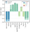 |
Fig. 7. Results of the Kendall τ rank correlation analysis between various predictors identified by Jaskot et al. 2024b and fesc values for both the entire LzLCS+ sample (88 sources) and the subsample of 51 galaxies. The hatched bar represents the refined subsample, while the other corresponds to the full sample. |
We first examined whether the reduction in sample size could explain the changes in Kendall τ rank correlation. To this end, we generated 200 random subsamples, each containing 51 sources (the same size as our subsample), and calculated the correlation coefficients for each. We found that, for most indirect indicators, the small decrease in correlation strength observed in the 51-source subsample can be attributed to the reduced sample size, suggesting that the weakening of these correlations is primarily a statistical effect. However, the observed change in correlation strength for Lyα EW is significantly larger than expected from sample size reduction alone. Furthermore, the small increase in correlation with MUV cannot be explained by the reduced sample size. Therefore, the variations in MUV and Lyα EW correlations likely reflect real physical differences, rather than merely the impact of a smaller sample size.
The absence of correlation with Lyα EW is surprising, as it has traditionally been considered one of the most solid indirect indicators. However, this view has recently been challenged. For example Citro et al. 2025, explored the connection between LyC leakage and Lyα emission in seven gravitationally lensed Lyα emitters at z ∼ 2. Their galaxies have similar properties to the LzLCS+ sample, and exhibit high Lyαfesc. Based on the relation calibrated on Lyα properties using the LzLCS+ sample, at least half of these sources should be classified as LCEs. In practice, none of them is detected in LyC with fesc ≤ 0.065. These findings suggest that the mechanisms governing LyC leakage may differ at high redshift, emphasizing the need for caution when applying low-redshift estimators to high-redshift sources. Indirect fesc estimators, such as Lyα EW, may have complex dependencies beyond the escape of LyC alone. It remains uncertain how changes in galaxy properties, which evolve withredshift, impact the diagnostic reliability for fesc.
4.2. A revised Cox model to predict fesc during the EoR
Having identified the subset of LzLCS+ galaxies that exhibit properties similar to high-redshift sources, we recalibrate the Cox proportional hazards model – a semi-parametric method that estimates the probability of an event (the detection of fesc) as a function of multiple variables (the various galaxy properties) Jaskot et al. 2024a,b – to more accurately predict fesc during the EoR. This selection provides a more reliable predictive framework, improving our ability to model the LyC escape properties of galaxies in the early Universe. In Appendix A, we outline the methodology presented by Jaskot et al. 2024a.
The concordance index, defined as a measure to assess goodness-of-fit, ranges from 0 (perfect disagreement) to 0.5 (perfectly random) to 1.0 (perfect concordance) (e.g., Davidson-Pilon 2019). From the models with a concordance coefficient C > 0.7 identified by Jaskot et al. 2024b, we selected those applicable to reionization-era sources. Specifically, we focused on two models that: (a) could be applied to all sources in our sample, and (b) did not include a morphology-dependent term. The exclusion of a morphology term aligns with the goal of the present study, which is to investigate whether LyC escape is influenced by the morphology of galaxies and the presence of mergers with high fesc. Since all the models in Jaskot et al. 2024b, including those with a morphology term, are statistically equivalent, this selection did not introduce any significant bias. Thus, we chose the ELG-EW and ELG-O32 models, which rely on key galaxy properties such as E(B–V), MUV, stellar mass, and, respectively, log10([O III]+Hβ) EWs and log10(O32).
The ELG-O32 model is our fiducial model, while the ELG-EW model is useful for sources where O32 cannot be computed due to the absence of one of the oxygen lines. Following the methodology outlined in Appendix A, we computed the baseline hazard function HF0(fabs) and the survival function S(fabs), which allowed us to estimate the median fabs (and consequently the median fesc), along with the 16th and 84th percentiles to establish confidence intervals for our predictions.
In Appendix A, we provide two tables (Tables A.1 and A.2), one for each model, which, following Jaskot et al. 2024b, provide the goodness-of-fit statistics for the subsample of LzLCS+ analogs, the fitted coefficients (βi) for each included variable, and the reference values  , which are the mean of the analogs xi values, where xi represents the input variable (MUV, E(B–V), log10(M*/M⊙), and log10(EW([O III]+Hβ)/Å) or log10(O32)). Finally, the tables list the baseline cumulative hazard function, HF0, calculated by the lifelines Cox model fitting routine Davidson-Pilon 2019 for each of the observed fesc values for LCEs in the LzLCS+ subsample.
Fig. 8 illustrates the comparison between the predicted fesc values using the full LzLCS+ sample and the analogs alone. Both predictions are consistent, with residuals showing similar trends across the two samples.
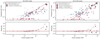 |
Fig. 8. Detected (or upper limit) fesc values versus the predicted fesc values ftom Cox models, calibrated using the full LzLCS+ sample and the subsample of galaxies resembling reionization-era sources. Left panel: Predictions using the ELG-EW model. Right panel: Predictions using the ELG-O32 model. The Cox models from Jaskot et al. 2024b are shown in blue, while predictions calibrated on the subsample are in red. Predictions applied to known LyC leakers at z ∼ 3 are also shown in red Vanzella et al. 2015, 2016; de Barros et al. 2016; Marques-Chaves et al. 2022; Fletcher et al. 2019; Kerutt et al. 2024. Upper limits are indicated with downward-pointing arrows. |
4.3. Applying the model to known leakers at z = 3
We further tested our model to assess its ability to predict fesc for galaxies at intermediate redshift by applying it to known LyC leakers at z ∼ 3. We compiled samples of z ∼ 3 leakers with reported detections of global absolute LyC values fesc that include all relevant variables: E(B-V), stellar mass, MUV, and either O32 or [O III]+Hβ EWs. This results in two distinct sets at z ∼ 3:
-
ELG-EW sample: This sample includes Ion2 (z = 3.2, fesc = 0.5–0.9, Vanzella et al. 2015, 2016; de Barros et al. 2016) and J1316+2614 (z = 3.6130, fesc ≈ 0.9, Marques-Chaves et al. 2022, 2024).
-
ELG-O32 sample: This sample includes Ion2, J1316+2614, two sources from Kerutt et al. 2024 observed in the JADES program (z = 3.46, fesc = 0.23 ± 0.05 and z = 4.43, fesc = 0.69 ± 0.10, respectively), and one source (z = 3.67, fesc = 0.31 ± 0.03) from the Lyman Continuum Escape Survey (LACES, Fletcher et al. 2019).
Our predictions, shown in Fig. 8, reveal a strong positive correlation with measured values at this intermediate redshift, with Pearson’s r= 0.812, indicating that our model effectively reflects the observed data. Although the p-value of 0.095 suggests marginal significance, this result reinforces the validity of our predictions. A primary limitation of our assessment is that we tested our model exclusively on strong leakers at z ∼ 3 (with fesc ≥ 0.2), as these are the only detections available with the complete dataset of indirect indicators required. Consequently, expanding the number of confirmed LyC leakers (or upper limits) at intermediate redshifts is essential to further refine of our model.
5. Results
5.1. The predicted fesc values
Using the revised ELG-O32 or ELG-EW models, we predicted the fesc values for most sources in our sample, successfully predicting all but nine of a total of 436 sources. The nine sources for which predictions were not made lack both the O32 ratio and the [O III] + Hβ EW. To obtain the most accurate estimates, we applied the revised ELG-O32 model (which has a concordance value of C = 0.83) whenever possible. For sources without detectable [O II] or [O III] lines, such as those of the EIGER sample, we applied the ELG-EW model (C = 0.79). Specifically, from the total sample of 427 sources with predicted fesc, we used the ELG-O32 model for 206 sources and the ELG-EW models for the remaining 221 sources. To ensure consistency between the two methods, we tested the correlation between the predicted fesc values from both models using the Spearman rank coefficient. We find a strong agreement (r = 0.86, p-value = 0.003). The distribution of predicted fesc values is shown in Fig. 9. Most of our galaxies exhibit modest inferred fesc values, generally around 0.10 or below. The average fesc for the sample, including the standard deviation as the 16th and 84th percentile values of the distribution, is  . This mean is skewed by the relatively high fesc values (> 0.4) inferred for a modest fraction (53 out of 427) of our sources. As a result, the median provides a more representative statistic, with a value of 0.04.
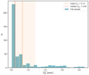 |
Fig. 9. Predicted fesc distribution for the analyzed sources at 5 ≤ z ≤ 7. The mean fesc of the sample, shown in red, is equal to |

The results align well with previous findings Mascia et al. 2023, 2024, both in terms of the shape of the distribution, the mean, and the median values. The models used in those studies were derived through linear regression, incorporating key predictors such as the O32 ratio, the Hβ EW, the β slope, and the UV half-light radius re. Our findings are also broadly consistent with Lin et al. 2024, who applied a logistic regression model to estimate the probability of a galaxy with MUV < −18 being an LCE, using MUV and β, and O32. They report that at z = 8, the average fesc varies with MUV, peaking at intermediate luminosities (−19 < MUV < −16) and reaching approximately 0.04 for brighter galaxies (MUV < −19). Similarly, Saxena et al. 2024 observed a comparable trend in a smaller sample of Lyα emitters, where a few sources exhibit a high fesc while the majority have fesc ≤ 0.10. Their model, based on the SPHINX20 simulation Choustikov et al. 2024, used six parameters (β, E(B-V), Hβ luminosity, MUV, R23, and O32) to predict LyC escape. It is important to note that all these methods are subject to their own caveats – whether in the treatment of upper limits, assumptions in simulations, or the handling of non-detections as non-LCEs. We note that the Choustikov et al. 2024 model, derived from simulated galaxies, substantially disagrees with the LzLCS+ sample, as shown by Jaskot et al. 2024b, and also diverges from Cox’s predictions for z ≥ 6 galaxies. Therefore, while these methods may yield similar population averages, they differ in their predictions for individual galaxies. Despite these differences, the methods demonstrate the strength of multivariate predictions and the value of combining different diagnostics to achieve a more robust understanding of LyC escape.
5.2. Merger fraction versus fesc
We examined the presence of merger and their connection to the predicted LyC escape fraction fesc for our sample of galaxies at z = 5 − 7. In Fig. 10 we color-coded the sources by the predicted fesc and find that high fesc sources are equally distributed between mergers and non-mergers. Specifically, we focus on fesc values exceeding 0.05, which is considered a reliable threshold for identifying strong LCEs, as suggested by Flury et al. 2022a. This threshold is further supported by our previous studies Mascia et al. 2023, 2024, which demonstrate that although there are uncertainties associated with these fesc values, those within this range are more reliable. Specifically, four of the 13 mergers in the Gold sample (31 ± 13%), 34 of 78 mergers in the Silver sample (44 ± 6%) and 107 of the 329 non-mergers (31 ± 3%) exhibit high LyC leakage. The fractions are all consistent across all groups, although the larger uncertainties in some subsets, particularly those with lower populations, prevent us from drawing firm conclusions. Notably, our conclusions remain unchanged even if we consider 0.1 as a threshold. In Fig. 11, we observe a potential connection between galaxy asymmetry (A) and fesc, with a Pearson correlation coefficient of r = −0.08 and a corresponding p-value of 0.17. Lower fesc values are associated with the full range of A values, whereas higher fesc values appear to be exclusively linked to galaxies with low asymmetry. It is important to note that the predictions for fesc in the two models we used are independent of any morphological terms, in contrast to other models previously employed Mascia et al. 2023, 2024; Jaskot et al. 2024a. Our results do not point to an increased fraction of high leakers in the merging systems, but rather indicate that the strongest leakers are preferentially compact.
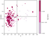 |
Fig. 10. Galaxies in our sample, color-coded by their predicted fesc values in three ranges: fesc < 0.02 (pale violet), 0.02 ≤ fesc ≤ 0.05 (magenta), and fesc > 0.05 (dark red). Point size corresponds to the predicted fesc, with larger points indicating higher values. |
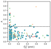 |
Fig. 11. Predicted fesc as a function of the A parameter. |
Recently, Bhagwat et al. 2024 investigated the link between morphology and LyC escape in the SPICE simulations. Their results support the idea that internal processes, rather than interactions, play a more critical role in driving LyC escape. Their simulations show that bursty stellar feedback can create low-density channels within galaxies that allow LyC photons to escape, regardless of whether the galaxy is undergoing a merger. This feedback-driven morphology, especially in dispersion-dominated systems, enhances LyC escape by producing irregular structures through internal processes rather than external interactions. This scenario is consistent with Flury et al. 2025 who present direct evidence for bursty star formation as a mechanism that enhances fesc in LCEs compared to non-LCEs.
These findings align with our results, which reveal that there is no relation between mergers and the predicted LyC escape. They support the view that LyC escape at these redshifts is predominantly governed by intrinsic factors such as the compactness of the star formation region. This observation is consistent with results from the LzLCS+ survey, where Flury et al. 2022a and Jaskot et al. 2024a identified compactness as a strong predictor of fesc, emphasizing its role as a key driver of the strong dependence of fesc on ΣSFR. Moreover, in a study of a leaker at z = 3.088, Gupta et al. 2024 discussed how optically thin channels, potentially created by merger-driven outflows, enable LyC escape. However, they caution that the complex outflow dynamics typical of high-redshift systems limits the likelihood that star-formation-driven feedback alone can create such channels.
Despite the strengths of our morphological classification, some limitations must be acknowledged. First, our classification is based on rest-frame UV imaging, which may not adequately capture the presence of merger signatures at z ∼ 7. Applying our classification to optical rest-frame morphology might have resulted in a different outcome, although Treu et al. 2023 report that the morphologies of the galaxy remain consistent across wavelengths from the optical rest-frame to UV. Another limitation arises from the uncertainty in classifying merger versus non-merger sources based solely on parametric classification. Although we conducted careful visual inspections of the sources in the Gold and Silver samples, this method may introduce bias and overlook small morphological features indicative of ongoing interactions or mergers.
As a final remark, it is important to consider the timing of mergers: what we identify in our sample could represent pre-merger conditions, or early stages of mergers, rather than fully merging systems. The formation of low-density channels that facilitate LyC escape may occur at later stages of the mergers, e.g., specifically during the coalescence phase (e.g., Conselice et al. 2000; Lotz et al. 2004; Pawlik et al. 2016), which are not captured by our classification scheme.
5.3. Merger fraction versus ξion
We also investigated the relationship between mergers and the ionizing photon production efficiency, ξion. Mergers are typically thought to temporarily increase star formation rates (SFRs) by compressing gas and triggering starbursts, which in turn could increase the production of ionizing photons (e.g., Barnes & Hernquist 1991; Mihos & Hernquist 1996). Higher SFRs typically correspond to younger, massive stellar populations, which emit more ionizing photons because of their high luminosity in both the UV and ionizing continua. A strong correlation between specific star formation rate (sSFR) and ξion has been observed Castellano et al. 2023, making sSFR one of the most reliable tracers of a galaxy’s ionizing efficiency, especially in the context of cosmic reionization (e.g., Llerena et al. 2025; Castellano et al. 2023). Witten et al. 2024, studying a sample of Lyα emitters at z > 7, further support this connection, demonstrating that mergers can trigger episodic bursts of star formation, which create low-density channels in the ISM, facilitating the escape of both Lyα and ionizing photons, and potentially enhancing ξion during merging events. However, compact low-mass galaxies with relatively high SFRs also exhibit elevated ξion Castellano et al. 2023, regardless of whether they are undergoing mergers.
Our results are presented in Fig. 12, where we plot the morphological parameters of our galaxies and color-code them according to their ξion. Galaxies with elevated ξion values are distributed across both merging and non-merging systems. Applying a threshold of log ξion = 25.5, we find that four of the 13 mergers in the Gold sample (31 ± 13%), 28 of 78 mergers in the Silver sample (36 ± 6%), and 133 of the 329 non-mergers (39 ± 3%) exhibit elevated ionizing emissivity. Although errors are large for samples exhibiting merger characteristics, the results suggest that elevated values of log ξion might be more common in compact, symmetric sources. These conclusions remain unchanged even if a threshold of 25.6 isconsidered.
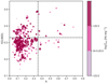 |
Fig. 12. Morphological parameters for galaxies in our sample, color-coded according to their measured log ξion values in three ranges: 23.5 ≤ log ξion ≤ 24.5 (pale violet), 24.5 ≤ log ξion ≤ 25.5 (magenta), and log ξion > 25.5 (dark red). Point size reflects the log ξion, with larger points indicating higher values. |
Additionally, the few sources with very high log ξion all exhibit very compact and symmetric morphologies in the rest-frame UV, reinforcing the idea that the production and escape of LyC radiation during the EoR are more closely related to compactness than to galaxy interactions or mergers.
6. Summary and conclusions
In this work, we assembled a sample of 436 spectroscopically confirmed sources at redshifts 5 ≤ z ≤ 7 from various JWST surveys, including EIGER, CEERS, DD-2750, and JADES. Using SED fitting with Prospector Johnson et al. 2021, we derived their physical properties such as stellar mass (M*), UV magnitude (MUV), UV β slope, dust reddening (E(B–V)), and specific star formation rate (sSFR). Emission line measurements enabled the determination of log ξion and other key properties, such as the O32 emission line ratio and the EW(Hβ) and EW([O III]). Finally, we classified the morphology of all systems using a well-tested morphological scheme according Dalmasso et al. 2024, which employ a combination of Asymmetry (A), Gini coefficient (G), and M20 parameters.
We compared the properties of these high-redshift sources to the LzLCS+ sample, and found that low- and intermediate-redshift LyC emitters are not always analogs for cosmic reionizers, exhibiting a diverse range of properties that only partially overlap with galaxies in the EoR. For this reason, we identified a subsample of the LzLCS+ survey sources, comprising 51 galaxies out of the original 88, which serve as the best analogs for the sources characterized during the EoR.
Although we restricted the LzLCS+ sample and created the subsample of “best analogs”, it is important to recognize that the definitive proof that this subsample truly represents the LyC emissivity of EoR galaxies and its correlation with other galaxies properties does not yet exist. The gaseous environments, in particular the ISM and the CGM, of low-z galaxies are most likely profoundly different from those of galaxies during the EoR. For example, even at cosmic noon, i.e., z ∼ 2 − 3, as reviewed by Tacconi et al. 2018, the gas fraction in star-forming disks is much higher – up to 80% – than in the local Universe, which can potentially have profound consequences for fesc. Figure 8 shows good agreement between the observed properties of galaxies at z ∼ 3 and those inferred from Cox models based on the LzLCS+, providing some reassurance that our sample of “best analogs” captures key features of the correlation between fesc and galaxy properties. However, it is important to remember that a final verification remains outstanding.
Assuming that the analogy holds, we use this subsample of analogs to propose two refined Cox models for predicting fesc during the EoR. These models are based on MUV, E(B-V), log10(M*), and ![Mathematical equation: $ \log_{10}(\text{ EW}([\text{ O}{\small { {\text{ III}}}}]+\text{ H}\beta)) $](/articles/aa/full_html/2025/09/aa53760-25/aa53760-25-eq8.gif) or log10(O32).The new models perform as well as, and in one case better than, the models originally proposed by Jaskot et al. 2024b, as demonstrated by the concordance index (C). To further test the robustness of our new models, we applied them to a small sample of confirmed LyC leakers at z ≈ 3 (the only ones with all necessary properties measured) and found that the models successfully predict their escape fractions.
or log10(O32).The new models perform as well as, and in one case better than, the models originally proposed by Jaskot et al. 2024b, as demonstrated by the concordance index (C). To further test the robustness of our new models, we applied them to a small sample of confirmed LyC leakers at z ≈ 3 (the only ones with all necessary properties measured) and found that the models successfully predict their escape fractions.
We applied the revised Cox models to infer fesc for our EoR galaxies. Combining these predictions with the identification of merging systems, we analyzed of the correlation between the presence of merger features and the production and escape of ionizing photons in galaxies during the EoR. Our main findings are as follows:
-
When applied to the large sample of galaxies observed during the EoR, our models confirm that the majority exhibit modest escape fractions, with a median of fesc ∼ 0.04 and an average fesc ∼ 0.13. The distribution of predicted escape fractions is highly skewed, with most objects showing small escape fractions and a tail extending to very high values. This finding reinforces previous conclusions by Mascia et al. 2024, suggesting that the galaxies currently probed (with MUV as faint as −18) contributed less than one third of the overall reionization budget. Further exploration of the fainter, low-mass galaxy population at high redshift is essential to fully understand their role in cosmic reionization.
-
Our analysis reveals no correlation between the predicted fesc and the presence of merger signatures. Most galaxies in the sample exhibit compact, symmetric morphologies rather than disturbed or irregular structures typically associated with mergers.
-
We find an increase of log ξion at fainter MUV, consistent with recent spectroscopic and photometric studies in literature (e.g., Simmonds et al. 2024; Prieto-Lyon et al. 2023; Llerena et al. 2025). We do not find any indication of an increased fraction of systems with high photon production efficiency among mergers. In contrast, there are indications that the most compact systems exhibit higher ξion values, suggesting a potential link between compactness and ionizing photon production.
Unfortunately, there are currently no systematic studies of the galaxy morphology of LyC leakers at low and intermediate redshifts, where direct detection of ionizing flux is feasible. Existing samples at low redshifts (e.g., the LzLCS+) may suffer from biases, as many sources were traditionally selected based on their compactness, which was thought to be related to the escape of LyC photons Izotov et al. 2018a. As noted in the Introduction, high LyC escape fractions have been reported for some merging systems at z = 1 Maulick et al. 2024 and at z = 3 Gupta et al. 2024; Yuan et al. 2024. Recently, Zhu et al. 2025 claimed that at z = 3, the majority of LyC leakers exhibit merging signatures. Such a result would be in stark contrast to our findings during the EoR. However, their sample includes only a few confirmed leakers, as many of the sources analyzed in their work are tentative detections. The few, solid LyC leakers at z = 3, such as Ion2, exhibit very compact morphology with no indication of merging activity. Additionally, their merging classification differs from those employed in our analysis, which could affect the outcome. We must also consider that at z ∼ 3, the transmission of the IGM becomes highly stochastic, allowing the detection of only the strongest LyC leakers.
This situation highlights the importance of building a statistically larger sample of leakers at z ∼ 3, with a broad range of fesc measurements (or upper limits). One example is the Parallel Ionizing Emissivity Survey (HST program 17147, PI C. Scarlata), conducted with HST to identify new LyC leakers at 3.1 < z < 3.5 among a sample of approximately 700 galaxies. An alternative approach will be employed by the LyC22 JWST program (GO 1869, PI D. Schaerer), which has obtained NIRSpec observations of known LCE. This program will provide the properties of the first robust sample of LCEs at the highest redshift where LyC can still be directly detected, offering a unique opportunity to systematically study their morphological properties. Crucially, the same dataset will enable the recalibration of Cox models at z ∼ 3. By bridging the gap between z = 0.3 and the EoR, this program will significantly enhance our understanding of the role of mergers and other processes in driving LyC escape, thereby improving the predictive power of fesc during reionization.
Acknowledgments
This work is based on observations made with the NASA/ESA/CSA James Webb Space Telescope. The data were obtained from the Mikulski Archive for Space Telescopes at the Space Telescope Science Institute, which is operated by the Association of Universities for Research in Astronomy, Inc., under NASA contract NAS 5-03127 for JWST. These observations are associated with programs GTO 1243, ERS 1345, DDT 2750, and GTO 1180, 1181, 3215, 1210, 1286. Funded by the European Union (ERC, AGENTS, 101076224). Views and opinions expressed are however those of the author(s) only and do not necessarily reflect those of the European Union or the European Research Council. Neither the European Union nor the granting authority can be held responsible for them. We acknowledge support from the INAF Large Grant 2022 “Extragalactic Surveys with JWST” (PI Pentericci). We acknowledge support from INAF Mini-grant “Reionization and Fundamental Cosmology with High-Redshift Galaxies” and from PRIN 2022 MUR project 2022CB3PJ3 - First Light And Galaxy aSsembly (FLAGS) funded by the European Union – Next Generation EU. RA acknowledges support of Grant PID2023-147386NB-I00 funded by MICIU/AEI/10.13039/501100011033 and by ERDF/EU, and the Severo Ochoa grant CEX2021-001131-S funded by MCIN/AEI/10.13039/50110001103. The project that gave rise to these results received the support of a fellowship from the “la Caixa” Foundation (ID 100010434). The fellowship code is LCF/BQ/PR24/12050015. LC acknowledges support from grants PID2022-139567NB-I00 and PIB2021-127718NB-I00 funded by the Spanish Ministry of Science and Innovation/State Agency of Research MCIN/AEI/10.13039/501100011033 and by “ERDF A way of making Europe”.
References
- Abraham, R. G., Tanvir, N. R., Santiago, B. X., et al. 1996, MNRAS, 279, L47 [Google Scholar]
- Abraham, R. G., van den Bergh, S., & Nair, P. 2003, ApJ, 588, 218 [NASA ADS] [CrossRef] [Google Scholar]
- Akritas, M. G., & Siebert, J. 1996, MNRAS, 278, 919 [NASA ADS] [CrossRef] [Google Scholar]
- Asthana, S., Haehnelt, M. G., Kulkarni, G., et al. 2024, ArXiv e-prints [arXiv:2409.15453] [Google Scholar]
- Atek, H., Labbé, I., Furtak, L. J., et al. 2024, Nature, 626, 975 [NASA ADS] [CrossRef] [Google Scholar]
- Bagley, M. B., Finkelstein, S. L., Koekemoer, A. M., et al. 2023, ApJ, 946, L12 [NASA ADS] [CrossRef] [Google Scholar]
- Barkana, R., & Loeb, A. 2001, Phys. Rep., 349, 125 [NASA ADS] [CrossRef] [Google Scholar]
- Barnes, J. E., & Hernquist, L. E. 1991, ApJ, 370, L65 [Google Scholar]
- Bassett, R., Ryan-Weber, E. V., Cooke, J., et al. 2019, MNRAS, 483, 5223 [Google Scholar]
- Bergvall, N., Leitet, E., Zackrisson, E., & Marquart, T. 2013, A&A, 554, A38 [NASA ADS] [CrossRef] [EDP Sciences] [Google Scholar]
- Bhagwat, A., Costa, T., Ciardi, B., Pakmor, R., & Garaldi, E. 2024, MNRAS, 531, 3406 [NASA ADS] [CrossRef] [Google Scholar]
- Bosman, S. E. I., Davies, F. B., Becker, G. D., et al. 2022, MNRAS, 514, 55 [NASA ADS] [CrossRef] [Google Scholar]
- Brammer, G. 2021, https://doi.org/10.5281/zenodo.7575984 [Google Scholar]
- Breslow, N. 1974, Biometrics, 30, 89 [Google Scholar]
- Byler, N., Dalcanton, J. J., Conroy, C., & Johnson, B. D. 2017, ApJ, 840, 44 [Google Scholar]
- Calabrò, A., Pentericci, L., Santini, P., et al. 2024, A&A, 690, A290 [NASA ADS] [CrossRef] [EDP Sciences] [Google Scholar]
- Calzetti, D., Meurer, G. R., Bohlin, R. C., et al. 1997, AJ, 114, 1834 [NASA ADS] [CrossRef] [Google Scholar]
- Calzetti, D., Armus, L., Bohlin, R. C., et al. 2000, ApJ, 533, 682 [NASA ADS] [CrossRef] [Google Scholar]
- Castellano, M., Belfiori, D., Pentericci, L., et al. 2023, A&A, 675, A121 [NASA ADS] [CrossRef] [EDP Sciences] [Google Scholar]
- Chabrier, G. 2003, PASP, 115, 763 [Google Scholar]
- Chisholm, J., Saldana-Lopez, A., Flury, S., et al. 2022, MNRAS, 517, 5104 [CrossRef] [Google Scholar]
- Choi, J., Dotter, A., Conroy, C., et al. 2016, ApJ, 823, 102 [Google Scholar]
- Choustikov, N., Katz, H., Saxena, A., et al. 2024, MNRAS, 529, 3751 [NASA ADS] [CrossRef] [Google Scholar]
- Citro, A., Scarlata, C. M., Mantha, K. B., et al. 2025, ApJ, 986, 184 [Google Scholar]
- Conselice, C. J., & Arnold, J. 2009, MNRAS, 397, 208 [NASA ADS] [CrossRef] [Google Scholar]
- Conselice, C. J., Bershady, M. A., & Jangren, A. 2000, ApJ, 529, 886 [NASA ADS] [CrossRef] [Google Scholar]
- Conselice, C. J., Bershady, M. A., Dickinson, M., & Papovich, C. 2003, AJ, 126, 1183 [CrossRef] [Google Scholar]
- Conselice, C. J., Yang, C., & Bluck, A. F. L. 2009, MNRAS, 394, 1956 [NASA ADS] [CrossRef] [Google Scholar]
- Costantin, L., Gillman, S., Boogaard, L. A., et al. 2025, A&A, 699, A360 [NASA ADS] [CrossRef] [EDP Sciences] [Google Scholar]
- Cox, D. R. 1972, J. Royal Stat. Soc. Ser. B (Methodological), 34, 187 [Google Scholar]
- Cox, T. J., Jonsson, P., Somerville, R. S., Primack, J. R., & Dekel, A. 2008, MNRAS, 384, 386 [NASA ADS] [CrossRef] [Google Scholar]
- Dalmasso, N., Calabrò, A., Leethochawalit, N., et al. 2024, MNRAS, 533, 4472 [NASA ADS] [CrossRef] [Google Scholar]
- Davidson-Pilon, C. 2019, J. Open Source Software, 4, 1317 [NASA ADS] [CrossRef] [Google Scholar]
- Dayal, P., Volonteri, M., Greene, J. E., et al. 2025, A&A, 697, A211 [NASA ADS] [CrossRef] [EDP Sciences] [Google Scholar]
- de Barros, S., Vanzella, E., Amorín, R., et al. 2016, A&A, 585, A51 [NASA ADS] [CrossRef] [EDP Sciences] [Google Scholar]
- D’Eugenio, F., Cameron, A. J., Scholtz, J., et al. 2025, ApJS, 277, 4 [Google Scholar]
- Dotter, A. 2016, ApJS, 222, 8 [Google Scholar]
- Eisenstein, D. J., Willott, C., Alberts, S., et al. 2023, ArXiv e-prints [arXiv:2306.02465] [Google Scholar]
- Ferland, G. J., Korista, K. T., Verner, D. A., et al. 1998, PASP, 110, 761 [Google Scholar]
- Fernández, V., Amorín, R., Firpo, V., & Morisset, C. 2024, A&A, 688, A69 [NASA ADS] [CrossRef] [EDP Sciences] [Google Scholar]
- Finkelstein, S. L., D’Aloisio, A., Paardekooper, J.-P., et al. 2019, ApJ, 879, 36 [Google Scholar]
- Finkelstein, S. L., Bagley, M., Song, M., et al. 2022a, ApJ, 928, 52 [CrossRef] [Google Scholar]
- Finkelstein, S. L., Bagley, M. B., Haro, P. A., et al. 2022b, ApJ, 940, L55 [NASA ADS] [CrossRef] [Google Scholar]
- Fletcher, T. J., Tang, M., Robertson, B. E., et al. 2019, ApJ, 878, 87 [Google Scholar]
- Flury, S. R., Jaskot, A. E., Ferguson, H. C., et al. 2022a, ApJ, 930, 126 [NASA ADS] [CrossRef] [Google Scholar]
- Flury, S. R., Jaskot, A. E., Ferguson, H. C., et al. 2022b, ApJS, 260, 1 [NASA ADS] [CrossRef] [Google Scholar]
- Flury, S. R., Jaskot, A. E., Saldana-Lopez, A., et al. 2025, ApJ, 985, 128 [Google Scholar]
- Gardner, J. P., Mather, J. C., Abbott, R., et al. 2023, PASP, 135, 068001 [NASA ADS] [CrossRef] [Google Scholar]
- Giavalisco, M., Dickinson, M., Ferguson, H. C., et al. 2004, ApJ, 600, L103 [NASA ADS] [CrossRef] [Google Scholar]
- Grogin, N. A., Kocevski, D. D., Faber, S. M., et al. 2011, ApJS, 197, 35 [NASA ADS] [CrossRef] [Google Scholar]
- Gupta, A., Trott, C. M., Jaiswar, R., et al. 2024, ApJ, 973, 169 [Google Scholar]
- Harrell, F. E., Califf, R. M., Pryor, D. B., Lee, K. L., & Rosati, R. A. 1982, JAMA, 247, 2543 [Google Scholar]
- Heckman, T. M., Sembach, K. R., Meurer, G. R., et al. 2001, ApJ, 558, 56 [Google Scholar]
- Inoue, A. K., Shimizu, I., Iwata, I., & Tanaka, M. 2014, MNRAS, 442, 1805 [NASA ADS] [CrossRef] [Google Scholar]
- Isobe, T., Feigelson, E. D., & Nelson, P. I. 1986, ApJ, 306, 490 [Google Scholar]
- Izotov, Y. I., Schaerer, D., Thuan, T. X., et al. 2016a, MNRAS, 461, 3683 [Google Scholar]
- Izotov, Y. I., Orlitová, I., Schaerer, D., et al. 2016b, Nature, 529, 178 [Google Scholar]
- Izotov, Y. I., Schaerer, D., Worseck, G., et al. 2018a, MNRAS, 474, 4514 [Google Scholar]
- Izotov, Y. I., Worseck, G., Schaerer, D., et al. 2018b, MNRAS, 478, 4851 [Google Scholar]
- Izotov, Y. I., Schaerer, D., Worseck, G., et al. 2020, MNRAS, 491, 468 [NASA ADS] [CrossRef] [Google Scholar]
- Izotov, Y. I., Guseva, N. G., Fricke, K. J., et al. 2021, A&A, 646, A138 [NASA ADS] [CrossRef] [EDP Sciences] [Google Scholar]
- Jaskot, A. E., Silveyra, A. C., Plantinga, A., et al. 2024a, ApJ, 972, 92 [NASA ADS] [CrossRef] [Google Scholar]
- Jaskot, A. E., Silveyra, A. C., Plantinga, A., et al. 2024b, ApJ, 973, 111 [NASA ADS] [CrossRef] [Google Scholar]
- Ji, Z., Giavalisco, M., Vanzella, E., et al. 2020, ApJ, 888, 109 [Google Scholar]
- Johnson, B. D., Leja, J., Conroy, C., & Speagle, J. S. 2021, ApJS, 254, 22 [NASA ADS] [CrossRef] [Google Scholar]
- Jung, I., Finkelstein, S. L., Arrabal Haro, P., et al. 2024a, ApJ, 967, 73 [NASA ADS] [CrossRef] [Google Scholar]
- Jung, I., Ferguson, H. C., Hayes, M. J., et al. 2024b, ApJ, 971, 175 [NASA ADS] [CrossRef] [Google Scholar]
- Kashino, D., Lilly, S. J., Matthee, J., et al. 2023, ApJ, 950, 66 [CrossRef] [Google Scholar]
- Katz, H., Ďurovčíková, D., Kimm, T., et al. 2020, MNRAS, 498, 164 [Google Scholar]
- Kerutt, J., Oesch, P. A., Wisotzki, L., et al. 2024, A&A, 684, A42 [NASA ADS] [CrossRef] [EDP Sciences] [Google Scholar]
- Koekemoer, A. M., Faber, S. M., Ferguson, H. C., et al. 2011, ApJS, 197, 36 [NASA ADS] [CrossRef] [Google Scholar]
- Le Reste, A., Cannon, J. M., Hayes, M. J., et al. 2024, MNRAS, 528, 757 [NASA ADS] [CrossRef] [Google Scholar]
- Leitherer, C., & Heckman, T. M. 1995, ApJS, 96, 9 [NASA ADS] [CrossRef] [Google Scholar]
- Li, W., Inayoshi, K., Onoue, M., & Toyouchi, D. 2023, ApJ, 950, 85 [Google Scholar]
- Lin, Y.-H., Scarlata, C., Williams, H., et al. 2024, MNRAS, 527, 4173 [Google Scholar]
- Llerena, M., Pentericci, L., Napolitano, L., et al. 2025, A&A, 698, A302 [NASA ADS] [CrossRef] [EDP Sciences] [Google Scholar]
- Lotz, J. M., Primack, J., & Madau, P. 2004, AJ, 128, 163 [NASA ADS] [CrossRef] [Google Scholar]
- Lotz, J. M., Jonsson, P., Cox, T. J., & Primack, J. R. 2008, MNRAS, 391, 1137 [Google Scholar]
- Madau, P., & Haardt, F. 2015, ApJ, 813, L8 [Google Scholar]
- Madau, P., Giallongo, E., Grazian, A., & Haardt, F. 2024, ApJ, 971, 75 [NASA ADS] [CrossRef] [Google Scholar]
- Mainali, R., Rigby, J. R., Chisholm, J., et al. 2022, ApJ, 940, 160 [NASA ADS] [CrossRef] [Google Scholar]
- Marques-Chaves, R., Schaerer, D., Álvarez-Márquez, J., et al. 2022, MNRAS, 517, 2972 [CrossRef] [Google Scholar]
- Marques-Chaves, R., Schaerer, D., Vanzella, E., et al. 2024, A&A, 691, A87 [NASA ADS] [CrossRef] [EDP Sciences] [Google Scholar]
- Mascia, S., Pentericci, L., Calabrò, A., et al. 2023, A&A, 672, A155 [NASA ADS] [CrossRef] [EDP Sciences] [Google Scholar]
- Mascia, S., Pentericci, L., Calabrò, A., et al. 2024, A&A, 685, A3 [NASA ADS] [CrossRef] [EDP Sciences] [Google Scholar]
- Matthee, J., Mackenzie, R., Simcoe, R. A., et al. 2023, ApJ, 950, 67 [NASA ADS] [CrossRef] [Google Scholar]
- Maulick, S., Saha, K., Kataria, M., & Herenz, E. C. 2024, ApJ, 972, 138 [Google Scholar]
- Merlin, E., Santini, P., Paris, D., et al. 2024, A&A, 691, A240 [NASA ADS] [CrossRef] [EDP Sciences] [Google Scholar]
- Mihos, J. C., & Hernquist, L. 1996, ApJ, 464, 641 [Google Scholar]
- Naidu, R. P., Tacchella, S., Mason, C. A., et al. 2020, ApJ, 892, 109 [NASA ADS] [CrossRef] [Google Scholar]
- Napolitano, L., Pentericci, L., Santini, P., et al. 2024, A&A, 688, A106 [NASA ADS] [CrossRef] [EDP Sciences] [Google Scholar]
- Oke, J. B., & Gunn, J. E. 1983, ApJ, 266, 713 [NASA ADS] [CrossRef] [Google Scholar]
- Pahl, A., Topping, M. W., Shapley, A., et al. 2025, ApJ, 981, 134 [Google Scholar]
- Pawlik, M. M., Wild, V., Walcher, C. J., et al. 2016, MNRAS, 456, 3032 [NASA ADS] [CrossRef] [Google Scholar]
- Pearson, W. J., Wang, L., Alpaslan, M., et al. 2019, A&A, 631, A51 [NASA ADS] [CrossRef] [EDP Sciences] [Google Scholar]
- Planck Collaboration VI. 2020, A&A, 641, A6 [NASA ADS] [CrossRef] [EDP Sciences] [Google Scholar]
- Prieto-Lyon, G., Mason, C., Mascia, S., et al. 2023, ApJ, 956, 136 [NASA ADS] [CrossRef] [Google Scholar]
- Rivera-Thorsen, T. E., Dahle, H., Gronke, M., et al. 2017, A&A, 608, L4 [NASA ADS] [CrossRef] [EDP Sciences] [Google Scholar]
- Rivera-Thorsen, T. E., Dahle, H., Chisholm, J., et al. 2019, Science, 366, 738 [Google Scholar]
- Robertson, B. E., & Schneider, E. 2013, Am. Astron. Soc. Meeting Abstr., 221, 207.02 [NASA ADS] [Google Scholar]
- Robertson, B. E., Ellis, R. S., Furlanetto, S. R., & Dunlop, J. S. 2015, ApJ, 802, L19 [Google Scholar]
- Roy, N., Henry, A., Treu, T., et al. 2023, ApJ, 952, L14 [NASA ADS] [CrossRef] [Google Scholar]
- Saldana-Lopez, A., Schaerer, D., Chisholm, J., et al. 2022, A&A, 663, A59 [NASA ADS] [CrossRef] [EDP Sciences] [Google Scholar]
- Saxena, A., Cryer, E., Ellis, R. S., et al. 2022, MNRAS, 517, 1098 [Google Scholar]
- Saxena, A., Bunker, A. J., Jones, G. C., et al. 2024, A&A, 684, A84 [NASA ADS] [CrossRef] [EDP Sciences] [Google Scholar]
- Schaerer, D., Izotov, Y. I., Verhamme, A., et al. 2016, A&A, 591, L8 [NASA ADS] [CrossRef] [EDP Sciences] [Google Scholar]
- Schaerer, D., Marques-Chaves, R., Barrufet, L., et al. 2022, A&A, 665, L4 [NASA ADS] [CrossRef] [EDP Sciences] [Google Scholar]
- Simmonds, C., Tacchella, S., Hainline, K., et al. 2024, MNRAS, 527, 6139 [Google Scholar]
- Spilker, J. S., Suess, K. A., Setton, D. J., et al. 2022, ApJ, 936, L11 [Google Scholar]
- Tacconi, L. J., Genzel, R., Saintonge, A., et al. 2018, ApJ, 853, 179 [Google Scholar]
- Toomre, A., & Toomre, J. 1972, ApJ, 178, 623 [Google Scholar]
- Treu, T., Calabrò, A., Castellano, M., et al. 2023, ApJ, 942, L28 [CrossRef] [Google Scholar]
- Vanzella, E., Guo, Y., Giavalisco, M., et al. 2012, ApJ, 751, 70 [NASA ADS] [CrossRef] [Google Scholar]
- Vanzella, E., de Barros, S., Castellano, M., et al. 2015, A&A, 576, A116 [NASA ADS] [CrossRef] [EDP Sciences] [Google Scholar]
- Vanzella, E., de Barros, S., Vasei, K., et al. 2016, ApJ, 825, 41 [NASA ADS] [CrossRef] [Google Scholar]
- Vanzella, E., Nonino, M., Cupani, G., et al. 2018, MNRAS, 476, L15 [Google Scholar]
- Verhamme, A., Orlitová, I., Schaerer, D., et al. 2017, A&A, 597, A13 [NASA ADS] [CrossRef] [EDP Sciences] [Google Scholar]
- Vulcani, B., Treu, T., Calabrò, A., et al. 2023, ApJ, 948, L15 [NASA ADS] [CrossRef] [Google Scholar]
- Wang, B., Heckman, T. M., Leitherer, C., et al. 2019, ApJ, 885, 57 [NASA ADS] [CrossRef] [Google Scholar]
- Wang, B., Heckman, T. M., Amorín, R., et al. 2021, ApJ, 916, 3 [NASA ADS] [CrossRef] [Google Scholar]
- Wise, J., Cen, R., et al. 2009, Am. Astron. Soc. Meeting Abstracts, 213, 348.04 [Google Scholar]
- Witten, C., Laporte, N., Martin-Alvarez, S., et al. 2024, Nat. Astron., 8, 384 [Google Scholar]
- Xu, X., Henry, A., Heckman, T., et al. 2023, ApJ, 943, 94 [NASA ADS] [CrossRef] [Google Scholar]
- Yuan, F.-T., Zheng, Z.-Y., Lin, R., Zhu, S., & Rahna, P. T. 2021, ApJ, 923, L28 [Google Scholar]
- Yuan, F.-T., Zheng, Z.-Y., Jiang, C., et al. 2024, ApJ, 975, 53 [Google Scholar]
- Yung, L. Y. A., Somerville, R. S., Finkelstein, S. L., et al. 2020a, MNRAS, 496, 4574 [NASA ADS] [CrossRef] [Google Scholar]
- Yung, L. Y. A., Somerville, R. S., Popping, G., & Finkelstein, S. L. 2020b, MNRAS, 494, 1002 [NASA ADS] [CrossRef] [Google Scholar]
- Zhu, S., Zheng, Z.-Y., Yuan, F.-T., Jiang, C., & Lin, R. 2025, ApJ, 982, L58 [Google Scholar]
Appendix A: Revised Cox models
The LzLCS+ results indicate that fesc correlates with various galaxy properties, including line-of-sight factors like HI covering fraction, dust attenuation, and Lyα escape fraction, as well as global properties such as O32 ratio and star formation rate surface density ΣSFR (e.g., Flury et al. 2022b; Chisholm et al. 2022; Saldana-Lopez et al. 2022; Xu et al. 2023). These correlations suggest that mechanical or radiative feedback may help create low optical depth sight lines that allow ionizing photons to escape. Nonetheless, the observed relationships between fesc and various galaxy properties show considerable scatter Wang et al. 2021; Flury et al. 2022b; Chisholm et al. 2022; Saldana-Lopez et al. 2022; Xu et al. 2023. This suggests that no single property can reliably predict fesc on its own, and a more accurate approach likely involves combining multiple factors.
Traditional methods like linear regression often fall short in handling censored data, which contain upper limits rather than precise measurements Mascia et al. 2023; Lin et al. 2024. To overcome these limitations, Jaskot et al. 2024a,b applied survival analysis techniques, particularly the Cox proportional hazards model Cox 1972, which is well suited for datasets with censored data.
In the Cox Model, the hazard function is expressed as:
 (A.1)
(A.1)
where h(t|x) is the hazard of detecting LyC, h0(t) is the baseline hazard function, and βi are the coefficients for the galaxy properties xi.
Using the absorbed fraction of LyC (fabs = 1 − fesc), the survival function S(fabs), representing the probability that fabs exceeds a given threshold, is:
![Mathematical equation: $$ \begin{aligned} S(f_{\text{abs}}) = \exp \left[ -H_{F_0}(f_{\text{ abs}}) \cdot \text{ ph}(x) \right], \end{aligned} $$](/articles/aa/full_html/2025/09/aa53760-25/aa53760-25-eq10.gif) (A.2)
(A.2)
where HF0(fabs) is the baseline cumulative hazard function:
 (A.3)
(A.3)
and ph(x) is the partial hazard function:
 (A.4)
(A.4)
The best-fit coefficients βi in the Cox proportional hazards model are determined by maximizing the partial likelihood, which compares ph(x) for each detection with the sum of ph(x) for all galaxies with higher fabs values Breslow 1974. The baseline cumulative hazard function HF0(fabs) is derived using Breslow’s estimator Breslow 1974, accounting for both detections and non-detections.
The median fabs is found when the survival function S(fabs) reaches 0.5, giving a 50% probability that the true fabs is above or below this value. Thus, the median predicted fesc is calculated as 1 − median fabs. The survival function also provides 1σ confidence intervals (where S(fabs) is 0.159 and 0.841), reflecting uncertainties in fesc due to observational scatter and intrinsic variability in the galaxy population.
The Cox model’s performance is evaluated using the concordance index (C) Harrell et al. 1982, which ranges from 0 (perfect disagreement) to 1 (perfect concordance):
 (A.5)
(A.5)
where nc, nd, and nt represent concordant, discordant, and tied pairs of observed and predicted values, respectively.
In Tables A.1 and A.2, we provide the information necessary to predict fesc using the models discussed in this paper.
Revised ELG-EW Model.
Revised ELG-O32 Model.
All Tables
Summary of JWST datasets and number of confirmed sources with redshifts 5 ≤ z ≤ 7 included in this study.
All Figures
|
Fig. 1. M1500 − z distribution for the 436 sources with 5 ≤ zspec ≤ 7 analyzed in this work. |
| In the text | |
|
Fig. 2. Stellar mass, log10(M⋆); UV magnitude, M1500; β slope; E(B–V); and log10(sSFR) for 436 sources in our sample, derived using Prospector. The ionizing photon production efficiency, log10ξion, was calculated for all sources with detectable Hα or Hβ using the relations proposed by Leitherer & Heckman 1995; Schaerer et al. 2016. The figure shows the median values along with their standard deviations (16th and 84th percentiles) for each distribution. |
| In the text | |
|
Fig. 3. Relation between log ξion and MUV. Each data point corresponds to an individual galaxy in our sample, with different symbols representing the various surveys. We include the curves from Simmonds et al. 2024; Pahl et al. 2025, as well as the relation from Llerena et al. 2025 at z ∼ 6. |
| In the text | |
|
Fig. 4. Visual representation of our classification results in the A vs f(G, M20) diagram. Symbols are the same as in Fig. 3. The two dashed lines indicate the threshold values determined from Eqs. (1) and (2). |
| In the text | |
|
Fig. 5. Non-merger and merger candidates from the various surveys considered in this study, separated into Silver and Gold samples. Each row shows two representative sources for each category: non-merging systems; Silver sample mergers (selected based on the f(G, M20) criterion, Eq. (1)); and Gold sample mergers (satisfying both f(G, M20) and A criteria, Eqs. (1) and (2)). The cutouts, in the F115W filter, show the rest-frame UV at the redshift of each galaxy. The source ID, redshift, asymmetry (A), and Gini-M20 (f(G, M20)) values are provided for each stamp. |
| In the text | |
|
Fig. 6. Comparison of galaxy properties between z ∼ 0.3 LyC emitters from the LzLCS+ Flury et al. 2022b and high-redshift sources, shown as a density plot. Panels show log M⋆ vs. β slope (top), MUV vs. β (middle), and E(B-V) vs. β (bottom). Of the 88 LyC emitters, 51 galaxies are identified as analogs to high-redshift sources, falling within the 99% confidence interval in all panels. Known LyC leakers at z ∼ 3 are also included from the literature: Ion1 Vanzella et al. 2012, Ion2 Vanzella et al. 2015, 2016; de Barros et al. 2016, Ion3 Vanzella et al. 2018, J1316+2614 Marques-Chaves et al. 2022, CDFS-6664 Yuan et al. 2021, LACES Fletcher et al. 2019, and samples from Kerutt et al. 2024 and Jung et al. 2024b. All the known leakers are color-coded by their log10(fesc). |
| In the text | |
|
Fig. 7. Results of the Kendall τ rank correlation analysis between various predictors identified by Jaskot et al. 2024b and fesc values for both the entire LzLCS+ sample (88 sources) and the subsample of 51 galaxies. The hatched bar represents the refined subsample, while the other corresponds to the full sample. |
| In the text | |
|
Fig. 8. Detected (or upper limit) fesc values versus the predicted fesc values ftom Cox models, calibrated using the full LzLCS+ sample and the subsample of galaxies resembling reionization-era sources. Left panel: Predictions using the ELG-EW model. Right panel: Predictions using the ELG-O32 model. The Cox models from Jaskot et al. 2024b are shown in blue, while predictions calibrated on the subsample are in red. Predictions applied to known LyC leakers at z ∼ 3 are also shown in red Vanzella et al. 2015, 2016; de Barros et al. 2016; Marques-Chaves et al. 2022; Fletcher et al. 2019; Kerutt et al. 2024. Upper limits are indicated with downward-pointing arrows. |
| In the text | |
|
Fig. 9. Predicted fesc distribution for the analyzed sources at 5 ≤ z ≤ 7. The mean fesc of the sample, shown in red, is equal to |
| In the text | |
|
Fig. 10. Galaxies in our sample, color-coded by their predicted fesc values in three ranges: fesc < 0.02 (pale violet), 0.02 ≤ fesc ≤ 0.05 (magenta), and fesc > 0.05 (dark red). Point size corresponds to the predicted fesc, with larger points indicating higher values. |
| In the text | |
|
Fig. 11. Predicted fesc as a function of the A parameter. |
| In the text | |
|
Fig. 12. Morphological parameters for galaxies in our sample, color-coded according to their measured log ξion values in three ranges: 23.5 ≤ log ξion ≤ 24.5 (pale violet), 24.5 ≤ log ξion ≤ 25.5 (magenta), and log ξion > 25.5 (dark red). Point size reflects the log ξion, with larger points indicating higher values. |
| In the text | |
Current usage metrics show cumulative count of Article Views (full-text article views including HTML views, PDF and ePub downloads, according to the available data) and Abstracts Views on Vision4Press platform.
Data correspond to usage on the plateform after 2015. The current usage metrics is available 48-96 hours after online publication and is updated daily on week days.
Initial download of the metrics may take a while.