© The Authors 2025

1. Introduction

The nature of the regeneration of the Sun’s large-scale poloidal magnetic field is a major outstanding problem in solar physics. Observations indicate that the poloidal component of the magnetic field at the surface of the Sun is crucial for the solar dynamo (Cameron & Schüssler 2015, 2020). The net amount of poloidal flux crossing the equator at the solar surface (Durrant et al. 2004) determines the polar magnetic fields at the following solar minimum, which plays a particularly important role in the amplitude of the subsequent solar cycle (Wang et al. 1989). Observations show that after emergence at the surface, the evolution of the magnetic field is governed by the Sun’s large-scale (differential rotation and meridional circulation in the surface flux transport model Yeates et al. 2023) and small-scale convective flows, with no systematic dependence on the sign of the magnetic field (Wang et al. 1989). Hence, after emerging at the surface, the magnetic field is not able to create a poloidal field in isolation; the poloidal magnetic field needs to be created during the flux-emergence process. The creation of the poloidal field during the magnetic flux emergence is indeed observationally well established and is a known consequence of Joy’s law (Hale et al. 1919).

Flux emergence is the process that carries the horizontal (longitudinal or latitudinal) magnetic field from the interior of the Sun across the photosphere in isolated active regions (Cheung & Isobe 2014; Weber et al. 2011; Caligari et al. 1995). The transport of the horizontal field across the photosphere creates radial magnetic flux of opposite polarities on either side of the emergence location. Hale’s law (Hale et al. 1919) states that during a solar cycle, each hemisphere has a preferred polarity for the radial magnetic flux on the leading side of the emergence, that is opposite in the two hemispheres, and reverses from one cycle to the next. Joy’s law states that, on average, the leading polarity is closer to the equator than the following polarity, and it was originally expressed in terms of the tilt angle of the line connecting the leading and following sunspots in white-light observations. It also states that active regions located at higher latitudes are more tilted than active regions near the equator. The combination of Hale’s law and Joy’s law implies a latitudinal separation of the two polarities of the azimuthally averaged radial field associated with the active region at the surface. This is equivalent to saying that the poloidal field appears at the surface during flux emergence. We investigate the extent to which this poloidal magnetic flux is generated beneath the surface and is then carried to the surface, or is generated at the surface by the emergence process itself.

Joy’s law is an empirical law that sets in during the emergence process (Kosovichev & Stenflo 2008; Schunker et al. 2020). This paper investigates its physical origins by comparing observations of the surface flows and the magnetic field as active regions emerge with numerical simulations of the flows and magnetic field as toroidal flux emerges.

2. Local surface electric fields associated with Joy’s law

The tilt angle of Joy’s law can be stated in terms of the relation between the latitudinal and longitudinal separation of the two polarities of the radial magnetic field associated with the emergence,

$$\begin{array}{c}\hfill {\displaystyle {\int }_A}{R}_{\odot }\theta B_r\mathrm{d}A=f({\theta }_0,t-t_{\mathrm{e}m})sin{\theta }_0{\displaystyle {\int }_A}{R}_{\odot }\varphi B_r\mathrm{d}A,\end{array}$$(1)

where B_r is the radial magnetic flux density of the flux-emergence event at the surface of the Sun, θ and ϕ are the co-latitude and longitude, θ₀ is the co-latitude at the location of the emergence, and the integral is evaluated over an area A encompassing the entire active region at the surface (see Figure 1), t_em is the emergence time, and t−t_em ≲ 2 days (the average duration of the active region emergence process, Weber et al. 2023). The factor f(θ₀,_t−_tem) describes the latitude and time dependence of the tilt angle in Joy’s law.

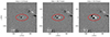Fig. 1. Example of the highest flux active region from the Helioseismic Emerging Active Region Survey (Schunker et al. 2016). The line-of-sight magnetic field is shown at three times during the emergence process. The emergence time, t = 0, is defined as when 10% of the maximum (over the 36 hours after the active region was given a NOAA number) magnetic flux has emerged. The red curve outlines the area A we used for the analysis of this active region emergence.

We used Faraday’s law, $\frac{\partial \mathbf{B}}{\partial t}=-c\mathrm{\nabla }\times \mathbf{E}$, to re-write the left-hand side of Equation (1) to obtain (we use cgs units througout this paper)

$$\begin{array}{cc}\hfill {\displaystyle {\int }_A}{R}_{\odot }\theta B_r\mathrm{d}A& ={\displaystyle {\int }_T}{\displaystyle {\int }_A}\theta R_{\odot }\frac{\partial B_r}{\partial t}\mathrm{d}A\mathrm{d}t\hfill \\ \hfill & ={\displaystyle {\int }_T}{\displaystyle {\int }_A}c{E}_{\varphi }\mathrm{d}A\mathrm{d}t+{\displaystyle {\int }_T}{\displaystyle {\oint }_{\delta A}}{R}_{\odot }c\theta \mathit{E}·\mathrm{d}\mathit{\ell }\mathrm{d}t,\hfill \\ \hfill \end{array}$$(2)

where the integrals are evaluated at the solar surface, in the flux emergence area, A, and over the emergence time t_em − 1 day< T <  t − t_em, c is the speed of light, and under the assumption that the area A is initially free of any substantial existing magnetic flux. We derived Eq. (2) using integration by parts (see the full derivation in Appendix A). We restricted our attention to the component of the electric field E associated with the flux emergence, E^FE, which includes the inductive effects of flows during the emergence. We used the observed sample of emerging active regions in the SDO Helioseismic Emerging Active Region Survey (Schunker et al. 2016), selected from Solar Dynamics Observatory Helioseismic and Magnetic Imager (SDO/HMI Scherrer et al. 2012) full-disk observations of the line-of-sight magnetic field, of active regions that emerge into the relatively quiet Sun without a substantial preexisting magnetic field. These flows were inferred from the travel times of waves that are sensitive to the top ≈2 Mm of the Sun, and they agree with local correlation-tracking methods with a correlation coefficient of about 0.93 in the quiet Sun (see Figure S1 in the Appendix of Birch et al. 2016). The Evershed flows associated with sunspot penumbrae can affect the inferred flows near sunspots (Braun 2019) and within sunspots (Schunker et al. 2008), but these flows only play a role after sunspots have formed, that is, after ≈2 days (see Gottschling et al. 2021) after the active region emergence begins.

Supporting this, Gottschling et al. (2022) have shown that the flows obtained by LCT largely reproduce the evolution of the surface field during the first 2 days. Observations show that at the photospheric level, flux-emergence events are localised in time and space (Fig. 1). Thus, the magnetic field associated with the flux emergence B^FE vanishes outside of A. Ohm’s law, $-c\mathbf{E}=\mathbf{U}\times \mathbf{B}-\frac{c}{\sigma }J$, then implies E^FE = 0 outside A. Thus, the expectation values of E^FE, ϕE^FE and θE^FE are 0 everywhere on the perimeter, δA, of A. This justifies ignoring the last term of Eq. (2), and we therefore obtain

$$\begin{array}{c}\hfill {\displaystyle {\int }_A}\overline{R_{\odot }\theta B_r}\mathrm{d}A={\displaystyle {\int }_T}{\displaystyle {\int }_A}\overline{c{E^{\mathrm{FE}}}_{\varphi }}\mathrm{d}A\mathrm{d}t,\end{array}$$(3)

where $\overline{X}$ indicates an average of X over many emergences. Similarly,

$$\begin{array}{c}\hfill {\displaystyle {\int }_A}{R}_{\odot }\overline{\varphi B_r}\mathrm{d}A=-{\displaystyle {\int }_T}{\displaystyle {\int }_A}\frac{c}{sin\theta }\overline{{E^{\mathrm{FE}}}_{\theta }}\mathrm{d}A\mathrm{d}t,\end{array}$$(4)

and Joy’s law (Eq. (1)) is then

$$\begin{array}{c}\hfill {\displaystyle {\int }_T}{\displaystyle {\int }_A}\overline{{E^{\mathrm{FE}}}_{\varphi }}\mathrm{d}A\mathrm{d}t=-f({\theta }_0,t-t_{\mathrm{em}}){\displaystyle {\int }_T}{\displaystyle {\int }_A}\overline{{E^{\mathrm{FE}}}_{\theta }}\mathrm{d}A\mathrm{d}t.\end{array}$$(5)

This averaging of E^FE is necessary because Joy’s law is a statistical effect. We also assumed that flux-emergence events are sufficiently localized in latitude to justify the approximation sinθ ≈ sinθ₀ and $sin{\theta }_0{\displaystyle {\int }_A}\frac{1}{sin\theta }{E^{\mathrm{FE}}}_{\theta }\mathrm{d}A\approx {\displaystyle {\int }_A}{E^{\mathrm{FE}}}_{\theta }\mathrm{d}A$. Equations (2), (3) and (5) are not surprising: Equations (2) and (3) state that the emerging flux comes from below the surface and is affected by flows and diffusion acting on the emerging magnetic field at the surface. Equation (5) then expresses Joy’s law in terms of local electric fields.

Still restricted to flux emergence, we can gain more insight from the observations by using Ohm’s law. We obtained the poloidal contribution from Eq. (3),

$$\begin{array}{cc}\hfill {\displaystyle {\int }_A}{R}_{\odot }\theta \overline{B_r}\mathrm{d}A& =-{\displaystyle {\int }_T}{\displaystyle {\int }_A}(\overline{U_r{B}_{\theta }}-\frac{\eta }{r}\frac{\partial [r\overline{B_{\theta }}]}{\partial r})\mathrm{d}A\mathrm{d}t\hfill \\ \hfill & +{\displaystyle {\int }_T}{\displaystyle {\int }_A}\overline{U_{\theta }{B}_r}\mathrm{d}A\mathrm{d}t\hfill \\ \hfill & -{\displaystyle {\int }_T}{\displaystyle {\int }_A}\frac{\eta }{r}\frac{\partial \overline{B_r}}{\partial \theta }\mathrm{d}A\mathrm{d}t\hfill \end{array}$$(6)

and the corresponding toroidal contribution

$$\begin{array}{cc}\hfill sin{\theta }_0{\displaystyle {\int }_A}{R}_{\odot }\varphi \overline{B_r}\mathrm{d}A& =-{\displaystyle {\int }_T}{\displaystyle {\int }_A}(\overline{U_r{B}_{\varphi }}-\frac{\eta }{r}\frac{\partial [r\overline{B_{\varphi }}]}{\partial r})\mathrm{d}A\mathrm{d}t\hfill \\ \hfill & +{\displaystyle {\int }_T}{\displaystyle {\int }_A}\overline{U_{\varphi }{B}_r}\mathrm{d}A\mathrm{d}t\hfill \\ \hfill & -{\displaystyle {\int }_T}{\displaystyle {\int }_A}\frac{\eta }{rsin\theta }\frac{\partial \overline{B_r}}{\partial \varphi }\mathrm{d}A\mathrm{d}t,\hfill \end{array}$$(7)

where we again assumed that sinθ ≈ sinθ₀ in A, and η is the Coulomb magnetic diffusivity, which is approximately 2 × 10⁸ cm²s⁻¹ in the photosphere (e.g. Sakai & Smith 2009). The corresponding diffusive length-scale over the 2-day emergence timescale is 59 km, which is almost an order of magnitude smaller than a SDO/HMI pixel (350 km). This implies that the contribution from ${\displaystyle {\int }_T}{\displaystyle {\int }_A}\frac{\eta }{rsin\theta }\frac{\partial \overline{B_r}}{\partial \varphi }\mathrm{d}A\mathrm{d}t$ and ${\displaystyle {\int }_T}{\displaystyle {\int }_A}\frac{\eta }{r}\frac{\partial \overline{B_r}}{\partial \theta }\mathrm{d}A\mathrm{d}t$ is small. More importantly, the arguments given in Cameron & Schüssler (2020) indicate that these two terms vanish (the same result can be obtained by applying the fundamental theorem of calculus and noting $\overline{B_r}=0$ on the boundary of A). Consequently, we have

$$\begin{array}{cc}\hfill {\displaystyle {\int }_A}{R}_{\odot }\theta \overline{B_r}\mathrm{d}A& =-{\displaystyle {\int }_T}{\displaystyle {\int }_A}(\overline{U_r{B}_{\theta }}-\frac{\eta }{r}\frac{\partial [r\overline{B_{\theta }}]}{\partial r})\mathrm{d}A\mathrm{d}t\hfill \\ \hfill & +{\displaystyle {\int }_T}{\displaystyle {\int }_A}\overline{U_{\theta }{B}_r}\mathrm{d}A\mathrm{d}t\hfill \end{array}$$(8)

and

$$\begin{array}{cc}\hfill sin{\theta }_0{\displaystyle {\int }_A}{R}_{\odot }\varphi \overline{B_r}\mathrm{d}A& =-{\displaystyle {\int }_T}{\displaystyle {\int }_A}(\overline{U_r{B}_{\varphi }}-\frac{\eta }{r}\frac{\partial [r\overline{B_{\varphi }}]}{\partial r})\mathrm{d}A\mathrm{d}t\hfill \\ \hfill & +{\displaystyle {\int }_T}{\displaystyle {\int }_A}\overline{U_{\varphi }{B}_r}\mathrm{d}A\mathrm{d}t.\hfill \end{array}$$(9)

We have kept the diffusive terms in Equations (8) and (9) for completeness, although they are likely to have only a minor contribution compared to the advective terms $\overline{U_r{B}_{\theta }}$ and $\overline{U_r{B}_{\varphi }}$, which have been shown to be substantial (MacTaggart et al. 2021).

The magnetic field at the surface of the Sun is largely radial, and we therefore treated the line-of-sight magnetic field observations from SDO/HMI as B_r. We used the surface horizontal flows (U_θ and U_ϕ) computed using helioseismic holography (Lindsey & Braun 2000) with an ≈6-hour cadence previously described in Birch et al. (2016) and Schunker et al. (2024). We also used the averaged the line-of-sight magnetic field maps over the corresponding time intervals. We note that $(U_r{B}_{\varphi }-\frac{\eta }{r}\frac{\partial r\overline{B_{\varphi }}}{\partial r})$ and $(U_r{B}_{\theta }-\frac{\eta }{r}\frac{\partial r\overline{B_{\theta }}}{\partial r})$ cannot be reliably obtained from current observations, mostly due to the 180-degree ambiguity in inferring the magnetic field orientation (e.g. Pevtsov et al. 2021). These terms can be determined as the differences between the measured terms in Equations (8) and (9), however.

Hereafter, we consider magnetic field and flow averages based on 182 isolated emerging active regions in the SDO HEARS (from Schunker et al. 2016, 2019), and drop the overbars. The left panel of Figure 2 shows the term on the left-hand side of Equation (9), sinθ₀∫_A R_⊙ϕB_rdA, and the second term on the right-hand side, ∫_T∫_AU_ϕB_rdAdt. The difference between them is equal to $({\displaystyle {\int }_T}{\displaystyle {\int }_A}{U}_r{B}_{\varphi }-\frac{\eta }{r}\frac{\partial [r{B}_{\varphi }]}{\partial r}\mathrm{d}A\mathrm{d}t)$, and it is substantial (≈4 × 10³⁰ Mx cm). In contrast, the term on the left-hand side of Equation (8), ∫_A R_⊙θB_rdA, is dominated by the contribution from ∫_T∫_AU_θB_rdAdt (shown by the very similar curves in the right panel of Fig. 2), so that the contribution from $({\displaystyle {\int }_T}{\displaystyle {\int }_A}{U}_r{B}_{\theta }-\frac{\eta }{r}\frac{\partial [r\overline{B_{\theta }}]}{\partial r}\mathrm{d}A\mathrm{d}t)$ is small. This term corresponds to the transport (by correlations between the magnetic field and flows or diffusion) of a north-south oriented magnetic field through the surface.

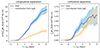Fig. 2. Average evolution of the toroidal and poloidal magnetic field due to flux emergences in the HEARS (Schunker et al. 2016) sample. The blue curves show sin(θ0)∫Aϕ R⊙BrdA (left panel) and ∫Aθ R⊙BrdA (right panel), where θ0 is the emergence colatitude. The orange curves show the contributions coming from ∫T∫AUϕBrdA dt and ∫T∫AUθBrdA dt in the left and right panels, respectively. The shaded regions show the respective 1σ error ranges. The error of the total and the error of the contributions from the surface flows are correlated. The difference between the blue and orange curves includes the effect of the contributions from horizontal magnetic flux being carried radially outward by small-scale radial flows. This component is small in the right panel, indicating that the field is east-west aligned before emergence, and only gains a north-south component due to north-south surface motions during the emergence process.

Thus, surprisingly, E^FE_ϕ comes largely from U_θB_r without a substantial contribution from U_rB_θ. This is consistent with the observation that, on average, emerging active regions initially have an east-west alignment, and the tilt develops over time (Kosovichev & Stenflo 2008; Schunker et al. 2020; Will et al. 2024). Figure 2 then implies that the interaction of the flows and magnetic field at the surface during the emergence process produces Joy’s law and the corresponding surface poloidal field. This is consistent with a simple estimate of the effect of the Coriolis force acting on a longitudinal flow, v_ϕ, moving the two polarities of an emerging bipole apart over the course of the two-day emergence period (Δ_t = 2 days). In this case, the tilt (in radians) is given

$$\begin{array}{cc}\hfill \mathrm{tilt}& =\frac{2\mathrm{\Omega }sin{\theta }_0{v}_{\varphi }\frac{{\mathrm{\Delta }}_t^2}{2}}{v_{\varphi }{\mathrm{\Delta }}_t}\hfill \\ \hfill & =\mathrm{\Omega }sin{\theta }_0{\mathrm{\Delta }}_t\hfill \\ \hfill & \approx \frac{2\pi sin{\theta }_0}{27\mathrm{days}}\times 2\mathrm{days}\hfill \\ \hfill & \approx 0.46sin{\theta }_0.\hfill \end{array}$$(10)

It is also consistent with the properties of the convective flows at the surface. For the active regions used in this study, the average separation in the longitudinal direction is about 40 Mm (Schunker et al. 2019). An east-west aligned tube emerging in a supergranule will have its leading and following polarities advected in opposite directions, with the velocity associated with the radial vorticity of the superganules, which is about 10 m/s (Langfellner et al. 2015), with the leading polarity being advected equatorward and the trailing polarity being advected poleward. The separation in longitude over two days then is about 3.5 Mm, which corresponds to a tilt angle of about 5°. This is comparable to what is expected from Joy’s law.

3. Flux emergence in dynamo simulations

The generation of a poloidal field at the solar surface can also be investigated using three-dimensional numerical magnetohydrodynamics simulations of magnetoconvection in a rotating shell. These global simulations do not yet reproduce the full range of dynamics of the Sun, but can nevertheless be used to investigate the key force balance and dynamo processes operating in stars. In this section, we use the simulation from Brun et al. (2022) and Noraz et al. (2024), which we previously used to investigate the toroidal flux budget (Finley et al. 2024). It is important to note that this simulation was not intended to model the Sun. It is part of a parameter study and represents a star that is 10% larger than the Sun and rotates three times faster. These numbers, however, only make sense in terms of the parameter study that was being performed, and we refer to Appendix B for a very brief description of the simulations and to Brun et al. (2022) and Noraz et al. (2024). We used the simulations as an example of magnetoconvection in a rotating spherical shell to investigate the appearance of the toroidal field at the surface of the simulation. The boundary conditions on the spherical surfaces were stress-free and impenetrable for the flow, and for the magnetic field, the interior was assumed to be a perfect conductor and the exterior a vacuum.

These simulations cannot expect to explicitly capture all the scales of the motions in a star. To make the problem tractable, the viscosity and diffusivity of the simulations are many orders of magnitude higher than the corresponding atomic values on the Sun. The simulations model the effects of the small-scale motions via enhanced turbulent viscosity and magnetic thermal diffusivities. The value we used for the magnetic diffusivity at the surface was η = 2195 km²/s. This value is comparable to what is required to transport the field from the small-scale granular convective motions that are missing in the simulations. In particular, the radial upflows associated with granulation on the Sun are U_r ≈ 1 km/s, and the size of granules is about 2000 km (so that UL ≈ 2000 km²/s.) The simulations directly capture the larger scales where the solar rotation has a direct impact via the Coriolis force, and they can simulate the effect of rotation on the flux as it emerges (Jouve et al. 2013). The equivalent to this diffusive flux through the surface in the simulation is on the Sun the flux due to the small-scale (granular) motions carrying the horizontal field through the surface.

It is a strong approximation of the simulations that they model the effects of granulation on the flux emergence in terms of a turbulent diffusivity. This is one of several ways in which the simulations are dissimilar to the Sun and other stars. Our purpose in studying the simulations is not to replicate flux emergence with the realism of high-resolution simulations (e.g., Cheung et al. 2007). We instead aim to investigate whether the main finding of Section 2, that the north-south separation of magnetic polarities is primarily driven by surface north-south motions acting on the radial field at the surface, also applies in a simplified dynamo simulation. This is a test of the robustness of the underlying physical processes. For this goal, it is not necessary for the simulations to reproduce flux emergence in full detail. We note that in our analysis of solar observations in Section 2, we did not make the approximation U′_r = 0 at the surface.

We considered 12 000 days of the simulation after the simulation had reached a statistically steady state. We analyzed the simulations on a grid with a resolution of 0.7° in longitude and latitude. To investigate flux emergence in this simulation, we relied on the fact that U_r = 0 on the outer boundary, implying that flux emergence in this simulation necessarily involvesdiffusion (Bondi & Gold 1950; Finley et al. 2024). The diffusion in the model represents turbulent diffusivity from smaller-scale convective motions on the Sun. The large-scale motions that feel the influence of the Coriolis force contribute additional turbulent diffusion.

We therefore identified the flux emergence at times and locations in the simulation where the rate at which the horizontal field $|B_h|=\sqrt{B_{\varphi }^2+B_{\theta }^2}$ diffuses across the upper boundary is high. Since Joy’s law is a statistical effect (Wang & Sheeley 1989), we followed (Schunker et al. 2016) and obtained the flow and magnetic field components of an average emergence. Since Joy’s law is a function of latitude, we averaged over the emergences located at each latitude in the simulation grid independently. We separated the time series into four segments of 3000 days. For each latitude and time segment, we found the n = 3000 times (t_i) and longitudes (ϕ_i) where the diffusion of horizontal flux through the surface ($|\frac{\eta }{r}\frac{\partial \left(r{B}_h\right)}{\partial r}|$) was largest. The value of η at the surface in the simulation is 2195 km²/s. The choice of n = 3000 is somewhat arbitrary. It corresponds to choosing one emergence per day on average. We then calculated the average of any of the flow or magnetic field terms, X,

$$\begin{array}{c}\hfill X(\theta ,\varphi ,t)=\frac{1}{n}\sum _{i=1}^{n}X(\theta ,\varphi +{\varphi }_i,t+t_i)\times P(X(\theta ,{\varphi }_i,t_i)),\end{array}$$(11)

where P(X)=1 if X is purely a component of the flow U, and $P(X)=\mathrm{sign}\left[\frac{\eta }{r}\frac{\partial \left(r{B}_{\varphi }\right)}{\partial r}\right]$ if X contains a component of the magnetic field B or U × B. This choice for P allows the average flows and magnetic fields to be determined regardless of the sign of the leading polarity.

In Figure 3 we show the ϕ and θ components of the surface electric field associated with emergences, calculated from Ohm’s law. The emergences in this ASH dynamo simulation are clearly similar to those on the Sun in that they are compact, and the electric field very quickly falls to zero away from the emergence event. This was achieved in the observations by choosing clean, isolated emergences, and was the basis for ignoring the contour integral in the derivation of, for example, Eq. (3). The electric field is also compact in the simulations, which justifies neglecting the term in our analysis of the simulations. The compactness of E_ϕ and E_θ implies that flux appears at the surface in the form of magnetic bipoles.

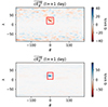Fig. 3. Properties of the average ϕ and θ components of the electric field associated with emergences at 20° latitude (λ) measured in the ASH simulation. The calculation of the electric field shown in this figure includes all diffusive and nondiffusive terms without approximations. The azimuthally averaged electric field from 40 days prior to the emergence was subtracted to concentrate on the field associated with the emergence. The red box shows the A we used to evaluate the integrals in Fig. 5.

Figure 4 shows some of the important terms for the flow and magnetic field averaged over the 12 000 emergences at a latitude of λ = 20°. At this latitude, magnetic flux preferentially emerges into regions with an existing strong radial field (Panel A). This largely masks the radial flux of the newly emerging bipole. The bipolar nature of the emergences is clearer at other latitudes, as shown in Appendix C in Figures C.1 and C.2. We comment that flux emergence also preferentially occurs on the Sun in the neighborhood of existing flux, and the system is then called an activity nest (Castenmiller et al. 1986). The U_ϕ component of the velocity at this latitude is dominated by a banana-like structure that is almost symmetric across the equator. This is the signature of a thermal Rossby wave, the dominant form of convection at low latitudes in most global simulations of the Sun (Käpylä et al. 2023). In these simulations, the thermal Rossby waves are confined to latitudes within λ ± 44°, corresponding to the tangent cylinder that is the projection of the Sun’s radiative interior along the rotation axis onto the upper boundary of the simulation. The average structure associated with the emergences at higher latitudes (|λ|< 44°, inside the tangent cylinder) is no longer dominated by thermal-Rossby waves. Panel A also implies that in the simulations, flux emergence tends to occur where there is preexisting radial flux.

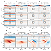Fig. 4. Properties of the average emergence at 20° latitude (λ) measured in the ASH simulation. The left panels (A) show the average radial magnetic field at the outer boundary associated with 12 000 emergence events (3000 from each of the four subsamples covering the simulation). All events were shifted in time and longitude to be centered at t = 0 and ϕ = 0. Column (B) shows the rate at which toroidal flux diffuses through the outer boundary. Column (C) shows Uϕ, and column (D) shows Uθ. The effects of differential rotation were removed in all cases by rotating each latitude according to its local rotation rate. The black boxes are centered on the emergence location. Quantities involving Ur are not shown because Ur = 0 on the outer boundary of the simulation. Panels E to H show insets of the same quantities at one day.

Comparing the magnitudes of the terms in Panel (A) and (B) of Figure 5 shows that E^FE_θ is always dominated by the explicit diffusive term (Panel A) that models the effect of the unresolved small-scale turbulent motions. Figure 5 (D) shows that in the northern hemisphere, the component of E^FE_ϕ generated by the north-south flows acting on the radial field associated during the emergence has the same sign as E^FE_θ. In the southern hemisphere, they have the opposite sign. This contribution to E^FE_ϕ corresponds to Figure 6. The emergence of the north-south field from below, shown in panel C, has mixed signs in each hemisphere. This is to be expected from turbulent processes, such as the alpha effect, operating in the simulated stellar interior.

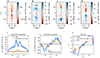Fig. 5. Terms contributing to the average cEFE as a function of central emergence latitude and time Panels A and B show the diffusive and advective contributions to cEFEθ, and panels C and D show the contributions to cEFEϕ. Here, U′ and B′ are the velocity and magnetic fields without their longitudinal means. Panels E and F show the contributions from Uϕ′Br′ and Uθ′Br′ as well as the total cEFEθ and cEFEϕ integrated from one day before emergence (t = −1 day) to one day after emergence (t = 1 day). The shaded regions show the 1σ error range, calculated from the four time-segments used in the analysis. Panel G shows Joy’s law based on the total longitudinal separation (the blue curve from panel E) and the total latitudinal separation (the blue curve from panel F), and Joy’s law based on the separation in latitude due to the latitudinal surface velocity acting on the radial field (the orange curve from panel F). The green line show Joy’s law derived from observations (e.g. Dasi-Espuig et al. 2010).

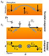Fig. 6. Sketch of the flows and their correlation with the magnetic field that lead to Joy’s law. In the first phase, the toroidal field is pushed through the surface by a radial upflow (upper panel). This creates radial field at the surface. Associated with the upflow is a horizontal outflow (middle panel), which advects the newly emerged magnetic bipoles, which further enhances the loss of toroidal field. The horizontally diverging material is acted on by the Coriolis force, so that the flows become helical. In particular, the Uϕ flow drives a flow in the north-south direction, Uθ, as shown in the lower panel. This north-south flow moves the preceding polarity toward the pole and the leading polarity towards the equator. The time evolution of the magnetic fields imply an electric fields EFE associated with the flux emergence. The corresponding contribution of flux emergence to the electromotive force is discussed in the text.

4. Babcock-Leighton alpha effect or Babock-Leighton delta effect?

As discussed in the introduction, Joy’s law is the essential process that introduces a poloidal component to the surface field driving the solar cycle, and the Babcock-Leighton dynamo model (Leighton 1969) captures the relevant physics. In this context, the appearance of poloidal flux at the solar surface during flux emergence, as a consequence of Joy’s law, has been called the Babcock-Leighton alpha effect.

While the assumptions underlying the mean-field framework, of which alpha is one part, do not strictly apply in the Sun, mean-field concepts can still be useful in giving a qualitative understanding of the most important physical processes. We also note that the form of the Babcock-Leighton dynamo equations corresponds to that of a mean-field dynamo (Stix 1974). The purpose of this section is to show that the poloidal field produced at the surface during flux emergence corresponds to a delta effect rather than an alpha effect.

The following arguments are slightly different for the case of the simulations and observations. The argument for the simulation begins by combining Eqs. (4) and (9) to obtain

$$\begin{array}{cc}\hfill {\displaystyle {\int }_T}{\displaystyle {\int }_A}\overline{{E^{\mathrm{FE}}}_{\theta }}\mathrm{d}A\mathrm{d}t& =\frac{1}{c}{\displaystyle {\int }_T}{\displaystyle {\int }_A}(\overline{U_r{B}_{\varphi }}-\frac{\eta }{r}\frac{\partial [r\overline{B_{\varphi }}]}{\partial r})\mathrm{d}A\mathrm{d}t\hfill \\ \hfill & -\frac{1}{c}{\displaystyle {\int }_T}{\displaystyle {\int }_A}\overline{U_{\varphi }{B}_r}\mathrm{d}A\mathrm{d}t.\hfill \end{array}$$(12)

In the numerical simulation, U_r vanishes identically at the upper boundary, and $\frac{1}{c}{\displaystyle {\int }_T}{\displaystyle {\int }_A}\overline{U_{\varphi }{B}_r}\mathrm{d}A\mathrm{d}t$ is small (see Fig. 5). Consequently, in the simulations,

$$\begin{array}{cc}\hfill {\displaystyle {\int }_T}{\displaystyle {\int }_A}\overline{{E^{\mathrm{FE}}}_{\theta }}\mathrm{d}A\mathrm{d}t& \simeq \frac{-1}{c}{\displaystyle {\int }_T}{\displaystyle {\int }_A}\frac{\eta }{r}\frac{\partial [r\overline{B_{\varphi }}]}{\partial r}\mathrm{d}A\mathrm{d}t,\hfill \end{array}$$(13)

where the magnetic diffusivity, η, used in the simulation is to be understood as the turbulent value of the diffusivity that is intended to model the effect of the granular-scale motions, including radial flows carrying flux through the solar surface.

In the context of solar observations, during flux emergence, the right-hand side of Eq. (12) corresponds to the emergence of toroidal field from below. In particular, the net $\overline{U_r{B}_{\varphi }}$ corresponds to emerging field being transported through the photosphere (Cameron et al. 2018). Flux emergence involves magnetic flux being carried across the surface by nonaxisymmetric (small-scale) flows. The net effect on the mean field is to remove flux from the solar interior and transport it into the atmosphere. The rate at which the subsurface toroidal flux is lost through the surface depends on the rate at which it is pushed through the surface by small-scale flows. As the field is pushed to the surface, a radial gradient of the toroidal field strength is created. Hence, at the surface, $⟨\overline{U_r{B}_{\varphi }}⟩$ is proportional to $⟨\frac{1}{r}\frac{\partial [r\overline{B_{\varphi }}]}{\partial r}⟩$ , where the overbars represent an ensemble average, and ⟨…⟩ represents an azimuthal average. This is to say that at the surface, the loss of toroidal flux through the surface due to small-scale motions is proportional to the radial gradient of the (axisymmetric) toroidal field on average, which is determined by the rate at which magnetic flux is advected to the surface from below. The constant of proportionality is called the turbulent diffusivity in the mean-field framework. The turbulent diffusivity is thus part of the parameterization of the effect on the mean-field of flux being carried across the surface by small-scale radial motions.

More formally, the entire right-hand side of Eq. (12) depends on the rate at which flux is pushed toward the surface from below, and hence, it is proportional to the surface value of $\frac{1}{r}\frac{\partial [r\overline{B_{\varphi }}]}{\partial r}$. In the context of the Babcock-Leighton model, the constant of proportionality is called the turbulent diffusivity, η_turb. Joy’s law, in the form given in Eq. (5), then yields

$$\begin{array}{cc}\hfill {\displaystyle {\int }_T}{\displaystyle {\int }_A}\overline{{E^{\mathrm{FE}}}_{\varphi }}\mathrm{d}A\mathrm{d}t& =-f({\theta }_0,t-t_{\mathrm{em}}){\displaystyle {\int }_T}{\displaystyle {\int }_A}\overline{{E^{\mathrm{FE}}}_{\theta }}\mathrm{d}A\mathrm{d}t\hfill \\ \hfill & =\frac{f({\theta }_0,t-t_{\mathrm{em}})}{c}{\displaystyle {\int }_T}{\displaystyle {\int }_A}\frac{{\eta }_{\mathrm{turb}}}{r}\frac{\partial [r\overline{B_{\varphi }}]}{\partial r}\mathrm{d}A\mathrm{d}t.\hfill \\ \hfill \end{array}$$(14)

Introducing the azimuthal mean of the surface quantities, denoted by the operator ⟨…⟩, we can now consider the effect of emergences at all longitudes within some latitudinal band [θ₀ : θ₀ + Δ_θ] during the time period T. We obtain

$$\begin{array}{cc}\hfill {\displaystyle {\int }_T}{\int }_{{\theta }_0}^{{\theta }_0+{\mathrm{\Delta }}_{\theta }}\overline{⟨{E^{\mathrm{FE}}}_{\varphi }⟩}\mathrm{d}\theta \mathrm{d}t& =\frac{f(\theta ,t-t_{\mathrm{em}})}{c}\hfill \\ \hfill & \times {\displaystyle {\int }_T}{\int }_{{\theta }_0}^{{\theta }_0+{\mathrm{\Delta }}_{\theta }}\frac{{\eta }_{\mathrm{turb}}}{r}\frac{\partial [r\overline{⟨B_{\varphi }⟩}]}{\partial r}\mathrm{d}\theta \mathrm{d}t.\hfill \end{array}$$(15)

Introducing the eletromotive force associated with flux emergence, 𝔈^FE = −c⟨E^FE⟩, we can write 𝔈^FE_ϕ in the form

$$\begin{array}{cc}\hfill {{\mathfrak{E}}^{\mathrm{FE}}}_{\varphi }& =b_{\varphi \varphi r}\frac{\partial [r⟨B_{\varphi }⟩]}{\partial r}.\hfill \end{array}$$(16)

The generation of 𝔈^FE_ϕ is not due to a subsurface alpha effect that generates a poloidal field beneath the surface. Instead, the north-south component of 𝔈^FE_ϕ is generated at the surface by correlations between the fluctuating components of U_θ and B_r. This process is physically different from the alpha effect. The fluctuating component of B_r is the direct consequence of the previous transport of toroidal flux through the surface, and it is hence proportional to $\frac{\partial r⟨B_{\varphi }⟩}{\partial r}$, where an integration over the time and space of the emergence is implied.

Equation (16) expresses the electromotive force due to flux emergence in terms of the mean-field framework. The coefficient b_ϕϕr contributes to the r component of δ (Schrinner et al. 2007) and is closely associated with the Rädler effect (Rädler 1969a, b; Rädler et al. 2003). We therefore suggest that the generation of poloidal flux in the Babcock-Leighton model corresponds to a delta effect rather than an alpha effect.

5. Discussion

The poloidal magnetic field at the surface of the Sun plays a crucial role in generating the toroidal field in the interior (Cameron & Schüssler 2015). This surface poloidal field is largely generated by flux emergence that statistically obeys Joy’s law (Wang et al. 1989). We have shown that the flows relevant for Joy’s law are the surface flows (Figure 2).

The physical processes for the generation of the poloidal flux we discussed can be understood by reference to Figure 6: Toroidal flux emerges in upflows that create bipoles of radial magnetic field. The surface flows have a radial vorticity due to the Coriolis force, and these vortical flows advect the two polarities differently in the latitudinal direction, producing Joy’s law (see also Roland-Batty et al. 2025).

Data availability

The data used from the ASH simulations are available from Open Research Data Repository of the Max Planck Society (Edmond) at https://doi.org/10.17617/3.H40YYT. The SDO/HMI observations used in this paper are available via the database repository http://jsoc.stanford.edu

Acknowledgments

The HMI data used are courtesy of NASA/SDO and the HMI science team. RHC acknowledges useful conversations with Pascal Demoulin and useful comments from a referee. RHC, ASB, AS, AJF and LG acknowledge support from the European Research Council (ERC) under the European Union’s Horizon 2020 research and innovation programme (grant agreement No 810218 WHOLESUN). ASB, AS, AJF acknowledge support from the Centre National d’Etudes Spatiales (CNES) Solar Orbiter, and the Institut National des Sciences de l’Univers (INSU) via the Programme National Soleil-Terre (PNST). AS acknowledges the French Agence Nationale de la Recherche (ANR) project STORMGENESIS #ANR-22-CE31-0013-01. HS is the recipient of an Australian Research Council Future Fellowship Award (project number FT220100330) and this research is partially funded by this grant from the Australian Government. HS, WRB and LG acknowledge support from the project “Preparations for PLATO asteroseismology” DAAD project 57600926. HS & WRB acknowledge the Awabakal people, the traditional custodians of the unceded land on which their research was undertaken. RHC conceived and led the research, analyzed the ASH simulations, and drafted the paper. HS analyzed HMI/SDO observations, helped conceive the study and drafted the paper. WRB tested the initial concept and reviewed drafts of the paper. ASB, AS and AF computed the ASH simulations, helped conceive the study and reviewed drafts of the paper. LG and ACB helped conceive the study and reviewed drafts of the paper.

References

Appendix A: Derivation of Equation 2 in the main text

We consider a flux emergence occurring inside a region of the solar surface A, during a time period T. We use B_r to denote the radial component of the magnetic field due to the emergence. Conservation of magnetic flux follows from the induction equation, and implies ∫_AB_rdA = 0 for all t ∈ T. Then

$$\begin{array}{cc}\hfill {\displaystyle {\int }_A}\theta R_{\odot }{B}_r\mathrm{d}A& ={\displaystyle {\int }_A}{R}_{\odot }\theta \mathbf{B}·\mathrm{d}\mathbf{A}\hfill \\ \hfill & ={\displaystyle {\int }_T}{\displaystyle {\int }_A}\theta R_{\odot }\frac{\partial \mathbf{B}}{\partial t}·\mathrm{d}\mathbf{A}\mathrm{d}t\hfill \\ \hfill & =-{\displaystyle {\int }_T}{\displaystyle {\int }_A}\theta R_{\odot }c\mathrm{\nabla }\times {\mathbf{E}}^{\mathrm{FE}}·\mathrm{d}\mathbf{A}\mathrm{d}t\hfill \\ \hfill & =-{\displaystyle {\int }_T}{\displaystyle {\int }_A}{R}_{\odot }c\mathrm{\nabla }\times \left(\theta {\mathbf{E}}^{\mathrm{FE}}\right)·\mathrm{d}\mathbf{A}\mathrm{d}t+{\displaystyle {\int }_T}{\displaystyle {\int }_A}{R}_{\odot }c\left(\mathrm{\nabla }\theta \right)\times {\mathbf{E}}^{\mathrm{FE}}·\mathrm{d}\mathbf{A}\mathrm{d}t\hfill \\ \hfill & ={\displaystyle {\int }_T}{\displaystyle {\int }_A}c({\widehat{\mathbf{e}}}_{\mathit{\theta }}\times {\mathbf{E}}^{\mathrm{FE}})·\widehat{{\mathbf{e}}_{\mathbf{r}}}\mathrm{d}A\mathrm{d}t-{\displaystyle {\int }_T}{\oint }_{\delta A}{R}_{\odot }c\theta {\mathbf{E}}^{\mathrm{FE}}·\mathrm{d}\mathit{\ell }\mathrm{d}t\hfill \\ \hfill & ={\displaystyle {\int }_T}{\displaystyle {\int }_A}c{E^{\mathrm{FE}}}_{\varphi }\mathrm{d}A\mathrm{d}t-{\displaystyle {\int }_T}{\oint }_{\delta A}{R}_{\odot }c\theta {\mathbf{E}}^{\mathrm{FE}}·\mathrm{d}\mathit{\ell }\mathrm{d}t\hfill \end{array}$$

Similarly

$$\begin{array}{cc}\hfill {\displaystyle {\int }_A}{R}_{\odot }\varphi B_r·\mathrm{d}A& ={\displaystyle {\int }_A}{R}_{\odot }\varphi \mathbf{B}·\mathrm{d}\mathbf{A}\hfill \\ \hfill & ={\displaystyle {\int }_T}{\displaystyle {\int }_A}\varphi R_{\odot }\frac{\partial \mathbf{B}}{\partial t}·\mathrm{d}\mathbf{A}\mathrm{d}t\hfill \\ \hfill & =-{\displaystyle {\int }_T}{\displaystyle {\int }_A}\varphi R_{\odot }c\mathrm{\nabla }\times {\mathbf{E}}^{\mathrm{FE}}·\mathrm{d}\mathbf{A}\mathrm{d}t\hfill \\ \hfill & =-{\displaystyle {\int }_T}{\displaystyle {\int }_A}{R}_{\odot }c\mathrm{\nabla }\times \left(\varphi {\mathbf{E}}^{\mathrm{FE}}\right)·\mathrm{d}\mathbf{A}\mathrm{d}t+{\displaystyle {\int }_T}{\displaystyle {\int }_A}{R}_{\odot }c\left(\mathrm{\nabla }\varphi \right)\times {\mathbf{E}}^{\mathrm{FE}}·\mathrm{d}\mathbf{A}\mathrm{d}t\hfill \\ \hfill & ={\displaystyle {\int }_T}{\displaystyle {\int }_A}\frac{c}{sin\theta }({\widehat{\mathbf{e}}}_{\mathit{\varphi }}\times {\mathbf{E}}^{\mathrm{FE}})·\widehat{{\mathbf{e}}_{\mathbf{r}}}\mathrm{d}A\mathrm{d}t-{\displaystyle {\int }_T}{\oint }_{\delta A}{R}_{\odot }c\varphi {\mathbf{E}}^{\mathrm{FE}}·\mathrm{d}\mathit{\ell }\mathrm{d}t\hfill \\ \hfill & =-{\displaystyle {\int }_T}{\displaystyle {\int }_A}\frac{c}{sin\theta }{E^{\mathrm{FE}}}_{\theta }\mathrm{d}A\mathrm{d}t-{\displaystyle {\int }_T}{\oint }_{\delta A}{R}_{\odot }c\varphi {\mathbf{E}}^{\mathrm{FE}}·\mathrm{d}\mathit{\ell }\mathrm{d}t\hfill \end{array}$$

Appendix B: Specification of parameters of the ASH simulation

The stellar dynamo simulation analysed in the paper has been computed by the ASH code (Brun et al. 2004) using the anelastic approximation of the magnetohydrodynamics equations. It is representative of a 1.1 M_⊙ rotating at 3 times the solar rate and produces a cyclic magnetic activity of about 5 yr. The inner and outer boundaries are impenetrable to flows and stress free. The magnetic field is matched to a potential field at the outer surface and the to a perfect conductor at the inner boundary.

The numerical resolution is (N_r × N_θ × N_ϕ) 769 × 512 × 1024. The thermal and magnetic Prandtl numbers are 0.25 and 1 respectively, the supercriticality of the convection Ra^*/Ra_c is 17.16 and the fluid Rossby number Ro_f is 0.54 (see Table 3 in Brun et al. (2022) for more details). The simulation has first been ran as a purely hydrodynamic model until it converged (Brun et al. 2017) and then a weak seed field was added and the simulation allowed to evolve for several decades in MHD/dynamo mode. The magnetic energy is saturated with a magnetic energy of about 9% of the total kinetic energy. About 74% of the kinetic energy is contained in its differential rotation component (see Table 5 of Brun et al. 2022), where full details of this simulation are provided.

Appendix C: Additional figures of averaged emergences in the ASH simulation at different latitudes

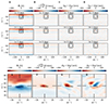Fig. C.1. Similar to Figure 4 except for the average emergence at 53° latitude (λ) in the ASH simulation.

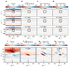Fig. C.2. Similar to Figure 4 except for the average emergence at 28° latitude (λ) in the ASH simulation.

All Figures

Fig. 1. Example of the highest flux active region from the Helioseismic Emerging Active Region Survey (Schunker et al. 2016). The line-of-sight magnetic field is shown at three times during the emergence process. The emergence time, t = 0, is defined as when 10% of the maximum (over the 36 hours after the active region was given a NOAA number) magnetic flux has emerged. The red curve outlines the area A we used for the analysis of this active region emergence.

In the text

Fig. 2. Average evolution of the toroidal and poloidal magnetic field due to flux emergences in the HEARS (Schunker et al. 2016) sample. The blue curves show sin(θ0)∫Aϕ R⊙BrdA (left panel) and ∫Aθ R⊙BrdA (right panel), where θ0 is the emergence colatitude. The orange curves show the contributions coming from ∫T∫AUϕBrdA dt and ∫T∫AUθBrdA dt in the left and right panels, respectively. The shaded regions show the respective 1σ error ranges. The error of the total and the error of the contributions from the surface flows are correlated. The difference between the blue and orange curves includes the effect of the contributions from horizontal magnetic flux being carried radially outward by small-scale radial flows. This component is small in the right panel, indicating that the field is east-west aligned before emergence, and only gains a north-south component due to north-south surface motions during the emergence process.

In the text

Fig. 3. Properties of the average ϕ and θ components of the electric field associated with emergences at 20° latitude (λ) measured in the ASH simulation. The calculation of the electric field shown in this figure includes all diffusive and nondiffusive terms without approximations. The azimuthally averaged electric field from 40 days prior to the emergence was subtracted to concentrate on the field associated with the emergence. The red box shows the A we used to evaluate the integrals in Fig. 5.

In the text

Fig. 4. Properties of the average emergence at 20° latitude (λ) measured in the ASH simulation. The left panels (A) show the average radial magnetic field at the outer boundary associated with 12 000 emergence events (3000 from each of the four subsamples covering the simulation). All events were shifted in time and longitude to be centered at t = 0 and ϕ = 0. Column (B) shows the rate at which toroidal flux diffuses through the outer boundary. Column (C) shows Uϕ, and column (D) shows Uθ. The effects of differential rotation were removed in all cases by rotating each latitude according to its local rotation rate. The black boxes are centered on the emergence location. Quantities involving Ur are not shown because Ur = 0 on the outer boundary of the simulation. Panels E to H show insets of the same quantities at one day.

In the text

Fig. 5. Terms contributing to the average cEFE as a function of central emergence latitude and time Panels A and B show the diffusive and advective contributions to cEFEθ, and panels C and D show the contributions to cEFEϕ. Here, U′ and B′ are the velocity and magnetic fields without their longitudinal means. Panels E and F show the contributions from Uϕ′Br′ and Uθ′Br′ as well as the total cEFEθ and cEFEϕ integrated from one day before emergence (t = −1 day) to one day after emergence (t = 1 day). The shaded regions show the 1σ error range, calculated from the four time-segments used in the analysis. Panel G shows Joy’s law based on the total longitudinal separation (the blue curve from panel E) and the total latitudinal separation (the blue curve from panel F), and Joy’s law based on the separation in latitude due to the latitudinal surface velocity acting on the radial field (the orange curve from panel F). The green line show Joy’s law derived from observations (e.g. Dasi-Espuig et al. 2010).

In the text

Fig. 6. Sketch of the flows and their correlation with the magnetic field that lead to Joy’s law. In the first phase, the toroidal field is pushed through the surface by a radial upflow (upper panel). This creates radial field at the surface. Associated with the upflow is a horizontal outflow (middle panel), which advects the newly emerged magnetic bipoles, which further enhances the loss of toroidal field. The horizontally diverging material is acted on by the Coriolis force, so that the flows become helical. In particular, the Uϕ flow drives a flow in the north-south direction, Uθ, as shown in the lower panel. This north-south flow moves the preceding polarity toward the pole and the leading polarity towards the equator. The time evolution of the magnetic fields imply an electric fields EFE associated with the flux emergence. The corresponding contribution of flux emergence to the electromotive force is discussed in the text.

In the text

	Fig. C.1. Similar to Figure 4 except for the average emergence at 53° latitude (λ) in the ASH simulation.
In the text

	Fig. C.2. Similar to Figure 4 except for the average emergence at 28° latitude (λ) in the ASH simulation.
In the text

References

- Birch, A. C., Schunker, H., Braun, D. C., et al. 2016, Sci. Adv., 2, e1600557 [CrossRef] [Google Scholar]
- Bondi, H., & Gold, T. 1950, MNRAS, 110, 607 [Google Scholar]
- Braun, D. C. 2019, ApJ, 873, 94 [NASA ADS] [CrossRef] [Google Scholar]
- Brun, A. S., Miesch, M. S., & Toomre, J. 2004, ApJ, 614, 1073 [Google Scholar]
- Brun, A. S., Strugarek, A., Varela, J., et al. 2017, ApJ, 836, 192 [Google Scholar]
- Brun, A. S., Strugarek, A., Noraz, Q., et al. 2022, ApJ, 926, 21 [NASA ADS] [CrossRef] [Google Scholar]
- Caligari, P., Moreno-Insertis, F., & Schussler, M. 1995, ApJ, 441, 886 [Google Scholar]
- Cameron, R., & Schüssler, M. 2015, Science, 347, 1333 [Google Scholar]
- Cameron, R. H., & Schüssler, M. 2020, A&A, 636, A7 [NASA ADS] [CrossRef] [EDP Sciences] [Google Scholar]
- Cameron, R. H., Duvall, T. L., Schüssler, M., & Schunker, H. 2018, A&A, 609, A56 [NASA ADS] [CrossRef] [EDP Sciences] [Google Scholar]
- Castenmiller, M. J. M., Zwaan, C., & van der Zalm, E. B. J. 1986, Sol. Phys., 105, 237 [CrossRef] [Google Scholar]
- Cheung, M.~C.~M., Schüssler, M., & Moreno-Insertis, F. 2007, A&A, 467, 703 [CrossRef] [EDP Sciences] [Google Scholar]
- Cheung, M. C. M., & Isobe, H. 2014, Living Reviews in Solar Physics, 11, 3 [NASA ADS] [CrossRef] [Google Scholar]
- Dasi-Espuig, M., Solanki, S. K., Krivova, N. A., Cameron, R., & Peñuela, T. 2010, A&A, 518, A7 [NASA ADS] [CrossRef] [EDP Sciences] [Google Scholar]
- Durrant, C. J., Turner, J. P. R., & Wilson, P. R. 2004, Sol. Phys., 222, 345 [Google Scholar]
- Finley, A. J., Brun, A. S., Strugarek, A., & Cameron, R. 2024, A&A, 684, A92 [NASA ADS] [CrossRef] [EDP Sciences] [Google Scholar]
- Gottschling, N., Schunker, H., Birch, A. C., Löptien, B., & Gizon, L. 2021, A&A, 652, A148 [NASA ADS] [CrossRef] [EDP Sciences] [Google Scholar]
- Gottschling, N., Schunker, H., Birch, A. C., Cameron, R., & Gizon, L. 2022, A&A, 660, A6 [Google Scholar]
- Hale, G. E., Ellerman, F., Nicholson, S. B., & Joy, A. H. 1919, ApJ, 49, 153 [NASA ADS] [CrossRef] [Google Scholar]
- Jouve, L., Brun, A. S., & Aulanier, G. 2013, ApJ, 762, 4 [NASA ADS] [CrossRef] [Google Scholar]
- Käpylä, P. J., Browning, M. K., Brun, A. S., Guerrero, G., & Warnecke, J. 2023, Space Sci. Rev., 219, 58 [CrossRef] [Google Scholar]
- Kosovichev, A. G., & Stenflo, J. O. 2008, ApJ, 688, L115 [NASA ADS] [CrossRef] [Google Scholar]
- Langfellner, J., Gizon, L., & Birch, A. C. 2015, A&A, 581, A67 [NASA ADS] [CrossRef] [EDP Sciences] [Google Scholar]
- Leighton, R. B. 1969, ApJ, 156, 1 [Google Scholar]
- Lindsey, C., & Braun, D. C. 2000, Sol. Phys., 192, 261 [Google Scholar]
- MacTaggart, D., Prior, C., Raphaldini, B., Romano, P., & Guglielmino, S. L. 2021, Nat. Commun., 12, 6621 [NASA ADS] [CrossRef] [Google Scholar]
- Noraz, Q., Brun, A. S., & Strugarek, A. 2024, A&A, 684, A156 [NASA ADS] [CrossRef] [EDP Sciences] [Google Scholar]
- Pevtsov, A. A., Liu, Y., Virtanen, I., et al. 2021, J. Space Weather Space Clim., 11, 14 [NASA ADS] [CrossRef] [EDP Sciences] [Google Scholar]
- Rädler, K. H. 1969a, Monats. Dt. Akad. Wiss, 11, 272 [Google Scholar]
- Rädler, K. H. 1969b, Monats. Dt. Akad. Wiss, 11, 194 [Google Scholar]
- Rädler, K.-H., Kleeorin, N., & Rogachevskii, I. 2003, Geophys. Astrophys. Fluid Dyn., 97, 249 [Google Scholar]
- Roland-Batty, W., Schunker, H., Cameron, R. H., et al. 2025, A&A, 700, A28 [NASA ADS] [CrossRef] [EDP Sciences] [Google Scholar]
- Sakai, J. I., & Smith, P. D. 2009, ApJ, 691, L45 [Google Scholar]
- Scherrer, P. H., Schou, J., Bush, R. I., et al. 2012, Sol. Phys., 275, 207 [Google Scholar]
- Schrinner, M., Rädler, K.-H., Schmitt, D., Rheinhardt, M., & Christensen, U. R. 2007, Geophys. Astrophys. Fluid Dyn., 101, 81 [Google Scholar]
- Schunker, H., Braun, D. C., Lindsey, C., & Cally, P. S. 2008, Sol. Phys., 251, 341 [Google Scholar]
- Schunker, H., Braun, D. C., Birch, A. C., Burston, R. B., & Gizon, L. 2016, A&A, 595, A107 [NASA ADS] [CrossRef] [EDP Sciences] [Google Scholar]
- Schunker, H., Birch, A. C., Cameron, R. H., et al. 2019, A&A, 625, A53 [NASA ADS] [CrossRef] [EDP Sciences] [Google Scholar]
- Schunker, H., Baumgartner, C., Birch, A. C., et al. 2020, A&A, 640, A116 [NASA ADS] [CrossRef] [EDP Sciences] [Google Scholar]
- Schunker, H., Roland-Batty, W., Birch, A. C., et al. 2024, MNRAS, 533, 225 [Google Scholar]
- Stix, M. 1974, A&A, 37, 121 [Google Scholar]
- Wang, Y. M., & Sheeley, N. R., Jr 1989, Sol. Phys., 124, 81 [NASA ADS] [CrossRef] [Google Scholar]
- Wang, Y. M., Nash, A. G., & Sheeley, N. R., Jr 1989, ApJ, 347, 529 [Google Scholar]
- Weber, M. A., Fan, Y., & Miesch, M. S. 2011, ApJ, 741, 11 [NASA ADS] [CrossRef] [Google Scholar]
- Weber, M. A., Schunker, H., Jouve, L., & Işık, E. 2023, Space Sci. Rev., 219, 63 [NASA ADS] [CrossRef] [Google Scholar]
- Will, L. W., Norton, A. A., & Hoeksema, J. T. 2024, ApJ, 976, 20 [Google Scholar]
- Yeates, A. R., Cheung, M. C. M., Jiang, J., Petrovay, K., & Wang, Y.-M. 2023, Space Sci. Rev., 219, 31 [CrossRef] [Google Scholar]