| Issue |
A&A
Volume 701, September 2025
|
|
|---|---|---|
| Article Number | A274 | |
| Number of page(s) | 27 | |
| Section | Planets, planetary systems, and small bodies | |
| DOI | https://doi.org/10.1051/0004-6361/202554116 | |
| Published online | 25 September 2025 | |
Impact of rotation on synthetic mass–radius relationships of two-layer rocky planets and water worlds
1
University of Bordeaux, CNRS, LAB, UMR 5804,
33600
Pessac,
France
2
LPC2E, OSUC, Univ Orleans, CNRS, CNES, Observatoire de Paris,
45071
Orleans,
France
★ Corresponding author: This email address is being protected from spambots. You need JavaScript enabled to view it.
Received:
12
February
2025
Accepted:
30
June
2025
Abstract
We analyze the effects of rotation on mass–radius relationships for single-layer and two-layer planets with a core and an envelope made of pure materials that includes iron, perovskite, and water in solid phase. The numerical surveys we adopted employ the DROP code updated with a modified polytropic equation of state (EoS). We investigated the flattening parameters, f, up to 0.2. In the mass range of 0.1 M⊕ ≲ M ≲ 10 M⊕, we find that the rotation systematically shifts the curves of composition towards larger radii and/or smaller masses. Relative to the spherical case, the equatorial radius, Req, is increased by about 0.36f for single-layer planets and by 0.30f to 0.55 f for two-layer planets (depending on the core size fraction, q, and the planet mass, M). Rotation is an additional source of confusion in deriving planetary structures, as the radius alterations are of the same order as i) current observational uncertainties for super-Earths and ii) EoS variations. We established a multivariate fit of the form Req(M, f, q), which enables a fast characterisation of the core size and rotational state of rocky planets and ocean worlds. We discuss how the observational data must be shifted in the diagrams to self-consistently account for an eventual planet spin, depending on the geometry of the transit (i.e. circular or oblate). A simple application to the recently characterised super-Earth candidate LHS 1140 b is discussed in this work.
Key words: equation of state / methods: numerical / planets and satellites: interiors / planets and satellites: oceans / planets and satellites: terrestrial planets
© The Authors 2025
 Open Access article, published by EDP Sciences, under the terms of the Creative Commons Attribution License (https://creativecommons.org/licenses/by/4.0), which permits unrestricted use, distribution, and reproduction in any medium, provided the original work is properly cited.
This article is published in open access under the Subscribe to Open model. This email address is being protected from spambots. You need JavaScript enabled to view it. to support open access publication.
1 Introduction
The great diversity of exoplanets, with more than 5700 objects detected over the last three decades, represents a remarkable challenge for models of the internal structure, as well as plausible scenarios of planetary formation, the mechanisms at work, and detection methods (Haswell 2010; Nielsen 2022). The opportunity to find planets resembling Earth, and even possibly hosting forms of life, has become an alluring reality (Léger et al. 2004; Schwieterman et al. 2018; Wandel 2018; Rigby & Madhusudhan 2024; Lichtenberg & Miguel 2025). When transit and Doppler spectroscopy are combined, the radius, R, and mass, M, of the planet are measured with a relatively good precision (e.g. Spiegel et al. 2014; Agol et al. 2021). The resulting mean massdensity 3M/4πR3 and the inspection of the planet position in pre-computed mass–radius diagrams bring informations in terms of their chemical and mineralogical composition. Unfortunately, these data are far from sufficient to infer a unique internal structure because the inverse problem is highly degenerate. There is a certain diversity of equations of state due to the variety of materials present at the period of formation and the thermodynamical conditions are complex. The number of internal layers is another important unknown. Key information linked to the planet environment and age of the system can also be considered to discriminate between plausible configurations and unlikely ones. In particular, the proximity of the parent star sets severe constraints in terms of chemical composition (Dorn et al. 2017; Brugger et al. 2017), stellar wind, instellation, and heat transport (Valencia et al. 2006; Wagner et al. 2012; Yunsheng Tian & Stanley 2013; Mousis et al. 2020; Aguichine et al. 2021; Haldemann et al. 2024), and tides towards synchronisation (Valencia et al. 2007b; Nettelmann et al. 2011; Kellermann et al. 2018). Obtaining realistic models that include all these ingredients at once are a formidable technical challenge.
To our knowledge, mass–radius relationships for planets (solid or even gaseous) are in general computed in the spherical limit. However, planets do rotate at varying periods and flatten. It is difficult to conceive that all exoplanets would end up as either perfect spheres with no proper spin or completely tidally locked with their parent star. Planets in our Solar System are good examples of objects exhibiting slow to moderate rotations. When the orbital separation is short, substantial three-dimensional (3D) deformations are expected (e.g. Chandrasekhar 1933b). For planets moving on large orbits, the spin-orbit resonnance may not be reached, depending on the age of the system. The timescale actually varies with the separation, a, and stellar mass, M⋆, as  (e.g. Goldreich & Peale 1968; Zahn 1989; Leconte et al. 2015; Barnes 2017). The accretion of gas and dust in a circumstellar disc is efficient in spinning up planetary embryos (e.g. Mitra 1977). Young planets are expected to rotate very fast, in particular, due to the accumulation of angular momentum from pebble accretion and collisions. Small-sized bodies such as asteroids are highly affected by stochastic collisions and may end up with small rotation periods of the order of a few hours (Farinella et al. 1992). In giant impact theory, the rotation period of the proto-Earth is estimated to 2.7-5.8 h (pre- and post-impacts) and the polar-to-equatorial axis ratio, Rpol/Req, of the spheroidal Earth is expected to have been well below unity, close to the mass-shedding limit and/or break-up velocity (de Meijer et al. 2013; Canup 2012).
Another motivation for considering rotation comes from the increasing interest for the detection of oblatness in transit lightcurves (Akinsanmi et al. 2020; Carado & Knuth 2020; Liu et al. 2025). The photometric signal from a transiting planet depends on the planet size relative to the star size and to the orbital separation (Haswell 2010). Again, the planet is generally assumed to be spherical, which means that area blocking the stellar flux towards the observer is a circular disc. The existence of oblat-ness introduces a bias when retrieving the planets parameters, in particular, the radius (Berardo & de Wit 2022). With present-day photometric sensitivity and time-sampling, the systematic detection of oblatness during the ingress and egress phases of transits is marginally accessible for gaseous planets, which represent the best targets (Zhu et al. 2014; Liu et al. 2024). In contrast, rocky planets and water worlds that have not reached synchronisation, yet still orbit at large separation are out of the range of detection for the transit method. In the perspective of finer measurements (in terms of timing and relative flux) and future instruments such as the Plato mission, there is great interest in anticipating and understanding the role of rotation in mass–radius relationships and in quantifying the additional level of confusion it brings to interpreting the data.
Estimating the change in the radius and/or mass of a selfgravitating fluid due to rotation is an old problem. For a homogenous spheroid with flattening,  , the equatorial radius is larger than for a sphere having the same mass by the quantity
  . In similar conditions, for a given equatorial radius, the mass of the rotating spheroid is smaller than for the sphere by ∆M ≈ -Mf. This means that for an uncompressible body with flattening f = 3% (a little bit higher than for Neptune and Uranus), the relative deviation in the radius reaches ∆Req/Req ≈ 1%, whose value is comparable to the precision obtained by the transit method. Solid planets are not homogeneous spheroids. The modification in the structure due to rotation has been treated in the limit of weak distorsion by Chandrasekhar (1933a) for a polytropic equation of state (EoS), where the pressure, P, and the mass-density, ρ, scale as P ∝ ργ. The result depends on the properties on Emden’s function at the equator (in particular, the non-analytical derivative) and especially on the polytropic exponent, γ, of the gas. As the rotation increases, the equatorial elongation changes faster than the pole contracts. For a given mass, the central density is slightly reduced for γ = 2, as described, for instance, by Williams (1988), Vavrukh & Dzikovskyi (2020) and Ricard & Chambat (2024). Here, we wish to quantify ∆Req and ∆M for rocky planets and water worlds and to compare these values with observational error bars, δR and δM. In this paper, we investigate the impact of rotation on synthetic, single-layer and two-layer planets with internal composition typical of the Earth (iron and silicate) and water-rich planets. The case of planets supporting an atmosphere is planned for another paper.
Authorising rotation renders the problem technically much more complex than in the static or spherical case, as there are two spatial coordinates to manage simultaneously, instead of a unique, radial variable. For this reason mainly, we deliberately abandoned certain ‘ingredients’ that are undoubtedly decisive in any realistic approach. We assumed single-layer and two-layer solid planets in rigid rotation, without any atmosphere. The radius is greatly changed in the presence of a relatively massive atmosphere (Adams et al. 2008; Howe et al. 2014). Regarding the EoS, there are several degrees of sophistication and realism, especially when the temperature is an explicit parameter (Swift et al. 2012; Hakim et al. 2018; Boujibar et al. 2020). For simplicity, we used a barotropic EoS appropriate to rocky or icy planets, in the form of the modified polytrope, according to Seager et al. (2007). This is a reliable approximation to more complex ansatz. In this context, different mineralogical compositions can be considered, from pure to impure materials. We selected only three kinds of materials, namely iron, silicate, and water (all in the solid phase). We also assumed that the parent star is far enough, therefore, we neglected the effects of tides (gravitational attraction and internal energy release) and irradiation that produce surface heating and trigger circulation caused by temperature imbalance at the surface (e.g. Auclair-Desrotour et al. 2024). We assumed the common hypothesis of rigid body rotation.
In Sect. 2, we briefly summarise the assumptions and equation set relevant to model a multi-layer planet in rotation, which are mostly described in Basillais & Huré (2021) and the main properties of the DROP code used to numerically solve the equilibrium on a cylindrical (R, Z)-grid (see also Huré & Hersant 2017; Huré et al. 2018). We focus on the specific link between the enthalpy, H, and the mass-density, ρ, associated with the EoS. Sections 3 and 4 are devoted to an exploration of the parameter space in the single-layer case and two-layer case, respectively. We note that there are two key parameters, namely the core fractional size, q ∈ [0,1], and the flattening, f = 1 - Rpol/Req. In particular (see Sect. I), we have taken the liberty to investigate the influence of rotation on mass–radius relationships well beyond the standard limit of slow rotations by considering flattening parameters, f, up to 0.2 (noting that simulations can go well above this level). We performed a global fitting procedure, leading to a general, fully reversible formula of the form Req = Req(M, q, f), mixing quadratic laws and a sigmoid. In Sect. 5, we discuss the diversity of structures in terms of δq and δf, compatible with observational error bars of δM for the mass and δReq in the radius. Although this is not the nominal target regarding our purpose, we also considered LHS 1140 b (Dittmann et al. 2017; Ment et al. 2019; Lillo-Box et al. 2020; Cadieux et al. 2024a), a potential ocean world that was recently modelled by Rigby & Madhusudhan (2024) and Daspute et al. (2024). The main results are summarised in the conclusion, including an example of a bias correction that is appropriate for both circular and oblate transits. A few perspectives and possible improvements of the present work are given throughout.
2 Single-layer and two-layer equilibrium configurations from the self-consistent field method and the DROP code
2.1 Equation set
The structure of an isolated, spherical planet in steady state is obtained, as in the case of stars, by integrating the 1D equation for hydrostatic equilibrium, where local gravity force balancing the pressure gradient is directly available from Gauss’s theorem. The integration proceeds from the centre or surface towards the opposite boundary and the shots are repeated until the boundary conditions are fulfilled, optionally with interior matching points (Cox & Giuli 1968; Haldemann et al. 2024). With this technique, it is relatively easy to incorporate various details in the physical and chemical processes, depending on the local conditions (Slattery 1977; Guillot 1999; Verhoeven et al. 2005; Seager et al. 2007; Rigby & Madhusudhan 2024). In the presence of rotation, the equation of hydrostatic equilibrium and the Poisson equation involve two spatial coordinates and the shooting methods are less direct. If the rotation rate, Ω, inside the planet depends only on the cylindrical distance, R, from the axis of rotation and the fluid is a barotrope (e.g. Amendt et al. 1989), then the two components of the Euler equation are the gradient of the following scalar field
 (1)
(1)
where  is the centrifugal potential, H = ∫ dP/ρ is the enthalpy, ρ is the mass density, P is the pressure, and Ψ is the gravitational potential, which obeys the Poisson equation,
 (2)
(2)
The problem then consists of finding the value of H that satisfies these two equations at each point in the fluid, and this is usually performed via an iterative procedure, known as the self-consistent field (SCF) method. The enthalpy, H, is first prescribed or guessed, then Ψ is computed from Eq. (2) by using ρ(H) and it is injected in Eq. (1) to get a new enthalpy. This new field is compared to the previous one, and the cycle is repeated until convergence. A broad scope of the literature has been devoted to the determination of the solutions for Eq. (1), in various contexts; in particular, assuming a polytropic EoS for the material, where P ∝ ργ (e.g. Hachisu 1986; Horedt 2004). A new difficulty arises when combining rotation and layering, due to the presence of mass-density jumps (e.g. Kiuchi et al. 2010; Schubert et al. 2011; Kadam et al. 2016; Basillais & Huré 2021; Houdayer & Reese 2023). Actually, when the body is made of L well-differentiated layers in total (and provided the two conditions above are still satisfied), then there is one Bernoulli equation per layer to consider because each layer has its own EoS. The gravitational potential is still defined by Eq. (2), but the second member becomes a piece-wise function. The pressure balance at each interface, Sl, bounding the layers l ∈ [1, L] and l + 1 is expressed as
 (3)
(3)
meaning that the knowledge of all interfaces is mandatory (layer L + 1 denotes the free space). In total, there are 2L + 1 equations to solve simultaneously. We proceeded according to Basillais & Huré (2021) by solving one Poisson equation per layer on a dedicated computational grid with appropriate boundary conditions, namely, ∆Ψl = 4πGρl, and the total potential Ψ is obtained by superposition. This is adapted to correctly treat mass-density jumps at the interface between layers.
As mentioned in the introduction, we consider single-layer and two-layer planets. For L = 2, the core (C) is layer 1, and the envelope (E) is layer 2 as depicted in Fig. 1. The equatorial and polar radius of the core are R1 and Z1, respectively, and we have R2 ≡ Req> ≥ R1 and Z2 ≡ Rpol ≥ Z1 for the envelope. Usually, rotation flattens the structure, so that we expect Zl ≤ Rl . The two layers are in rigid rotation at the same rate Ω.
2.2 The modified polytropic EoS and the selection of mineralogical compositions for solid planets
As the diversity of planetary interiors is wide, the coverage in mass-density, pressure, and temperature must be sufficient (e.g. Yunsheng Tian & Stanley 2013; Hakim et al. 2018; Boujibar et al. 2020; Haldemann et al. 2020). For telluric and ocean planets with masses in the range of 0.1 M⊕ to 10 M⊕, different variations of the EoS can be selected (e.g. Grasset et al. 2009; Spiegel et al. 2014; Ricard & Chambat 2024); see Sect. I. These are generally combinations of experimental data and theoretical calculations, consisting of piece-wise functions and tables of data specific for various phases. Our primary objective is to test the role of rotation and to simplify the problem as much as possible. In this context, we work with the barotropic EoS given by Seager et al. (2007), namely,
 (4)
(4)
where ρs is the mass-density at null pressure, while K and m are constants1. This analytical model works for several types of solid materials, in particular for water, silicates and iron, and it includes quantum effects important at very high pressures (Zapolsky & Salpeter 1969). It is well suited to bodies with central pressures from 1011 to 1013.5 dyn/cm2, expected for the mass range of interest here (Cox & Giuli 1968). More details are given in Sect. 3.4.
The parameters m, ρs, and K needed in Eq. (4) are listed in Table 1 for solid iron (I), perovskite (P), and water (W), following Seager et al. (2007). The table also contains the index n and the exponent  corresponding to the high-pressure limit. Regarding water, we are aware that ρs = 1.46 g/cm3 is larger than the standard values for ice and liquid phase in standard conditions; however, we followed the authors’ prescription for the sake of consistency.
If we consider only configurations where ρs(E) < ρs(C), including the unrealistic case of an iron core and a water envelope, there are six different possibilities:
C ∈ {I, P, W} for single-layer planets,
CE ∈ {IP, IW, PW} for two-layer planets.
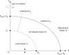 |
Fig. 1 Typical configuration and notations for a rotating system made of L = 2 differentiated layers: the core (C) as layer 1, and the envelope (E) as layer 2. The polar radius is Rpol ≡ Z2 and the equatorial radius is Req ≡ R2. All layers rotate at the same rate Ω around the Z-axis. |
2.3 The associated enthalpy
With respect to a polytropic EoS where P ∝ ργ and  , the bimodal prescription advantageously incorporates the uncom-pressible case n = 0 (i.e. γ → ∞) at vanishing pressure and a compressible case at high pressure, with
  . With Eq. (4), this change is especially significant in terms of the associated enthalpy H required in Eq. (1), as we have
 (5)
(5)
Unfortunately, a close form for H exists only for certain values of m. For instance, for  , the enthalpy is of the form H ~ ρ - const. × ln ρ. In the general case, H is given by
 (6)
(6)
where 2F1 denotes the Gauss hypergeometric function, and
 (7)
(7)
The non-linear change of variable (a Pfaff transformation) ensures that the hypergeometric series unconditionally converges since ρ ≥ ρs in the structure. It can be verified that, in these conditions, H(ρ) remains bijective, and it can therefore be inverted to get ρ(H). This inversion, which is accomplished by numerical means, is unavoidable since ρ is directly required to get the potential Ψ from the Poisson equation. The integration constant in Eq. (6) is of fundamental importance (there is one such constant per layer). It represents the enthalpy of the material at zero pressure, namely, for u = 0. If we define
 (8)
(8)
where ρ0 is, for instance, the largest value in the actual layer, then u0 = 1 - A and so the integration constant in Eq. (6) is
 (9)
(9)
Data⋆ for the modified EoS from Seager et al. (2007) according to Eq. (4).
2.4 Simulations of rotating two-layer planets at equilibrium with the updated DROP code
We use the DROP code to determine numerically the equilibrium state of a rotating body made of L layers (Basillais & Huré 2021) from the SCF method. The code is scale-free. In particular, we set ρ̃ = ρ/ρ0 for the mass density, and H̃ = H/H0 for the enthalpy, where ρ0 and H0 is specific to each layer. In the new version of the code, the modified polytropic EoS defined by Eq. (4) is implemented. The critical point is the automatic detection, at each step of the SCF-cycle, of the core-envelope interface S1 where Eq. (3) has to be fulfilled (see Fig. 1). Running a simulation with the DROP code requires three input parameters for L = 2:
the flattening parameter f = 1 - Rpol/Req ≥ 0,
the parameter
 , which sets the top-to-bottom mass-density ratio in the surface layer,
the relative size of the core q = Z1/Rpol along the Z-axis.
For a single-layer planet, A is basically the surface-to-centre mass density ratio and the last parameter is useless. The value of this parameter mostly determines the mass of the planet. For A - 0.3-0.85, we typically scan two decades in mass around one Earth mass, depending on the composition.
At convergence, the code delivers the enthalpy at equilibrium, Hl(R, Z), for each layer l = {1,2}, the interface, S1 and S2, in the form of discrete values, {Ri, Zi}, the rotation rate Ω, and the equatorial radius Req. From these data, we can compute the mass, Ml, of each layer, the total mass, M, the core mass-fraction, M1/M, the central pressure, Pc, the rotation period, T, and so on (see below). The accuracy of simulations is mainly controlled by the numerical resolution. We work with N + 1 = 129 grid nodes per direction, with uniform spacing. This is a moderate resolution. As the quadrature and finite difference schemes are second-order accurate in the unit-square grid, the relative precision in output quantities (mass, volume, virial parameter, etc.) is 1/N2 ≈ 10-4, typically. Most outputs are given with five digits.
2.5 An example of simulation
We show in Fig. 2 the pressure and mass-density profiles obtained for a two-layer planet made of an iron core and a perovskite envelope, namely, CE=IP. For this run, we take q = 0.5 and f = 0.05. The last parameter A ≈ 0.697 has been selected such that we get a planet with M ≈ 1 M⊕. Thus, this example represents a very simplified Earth, but with flattening parameter, f, comparable to Jupiter’s value (instead of ≃ 0.003). We see the smooth connection of the pressure at the interface, while the mass-density undergoes a jump, as expected. The ouput data are gathered in Table 2. The resulting equatorial radius is about 6346 km, and this is 6029 km at the pole. The rotation period is about 6 h 22 min.
2.6 Sampling for the numerical surveys: Tables
We have run the DROP code in the same conditions as in the previous example, by varying f, A, and q independently to each other. Given the moderate resolution (see above), a good compromise between the computing time and the quality of the data on output is obtained with the following samplings:
f ∈ [0,0.2], with ∆ f = 0.025 (f = 0 is for the static case),
A ∈ [0.05,0.95] with ∆A = 0.025,
q ∈ [0,1] for two-layer planets, with ∆q = 0.1.
This represents 171 runs for a single-layer planet, and 1536 runs in a two-layer case. As we have five different configurations (see Sect. 2.4), the number of runs amounts to 5130 in total. The list of input/output is given in the Appendix A together with a sample of data obtained for a water planet and for a IW planet and q = 0.5, with f = 0.1 in both cases. The full tables obtained for the six types of planets are available in electronic form on Zenodo2.
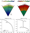 |
Fig. 2 Normalised pressure (left) and mass-density (right) in colour code (top) close to the pole and to the equator for a two-layer, IP planet computed with the DROP code. The input and output parameters are in Table 2. Profiles along the rotation axis (spherical radius r ≡ Z) and along the equator (r ≡ R) are also shown (bottom). |
3 Results in the single-layer case
Before considering configurations with L = 2, it is instructive to examine first the case where the planet is a single-layer body made of pure material, namely, C ∈ {I,P,W}. The mass–radius relationships obtained for f ∈ {0,0.1,0.2} are displayed in Fig. 3. In the static case, we have Req(W) > Req(P) > Req(I) for a given mass, which is expected from the mass density of the species. We find that:
decreasing ρs shifts the pure-composition lines quasihorizontally, towards low masses (i.e. a left shift in the plane),
decreasing the constant K-m shifts the pure composition lines towards large radii and high masses (a rightward and upward shift),
decreasing the power-law index m has a similar effect as decreasing the gaz constant.
In the graph, we have also reported the semi-empirical mass– radius relationship computed in Zeng et al. (2016) based on the preliminary reference Earth model (Dziewonski & Anderson 1981), the data computed by Haldemann et al. (2020) from the AQUA-EoS for water (assuming a 300 K surface temperature), and the results by Fortney et al. (2007) for pure water and pure silicate planets. Given the differences in the EoS and models of internal structure with these authors (explicit treatment of temperature and heat transport mainly), the comparisons with these authors are indeed satisfactory in the spherical case. Besides, we have checked that the agreement with Fortney et al. (2007) is much better for the water line by setting ρs ≃ 1 g/cm3 in the code.
3.1 Trends and fits
We observe that changing f at constant mass (radius) shifts the equatorial radius (mass, respectively) towards larger (lower, respectively) values, which is the consequence of the deficiency of matter along the rotation axis, i.e. Rpol < Req. The massradius relationships obtained for different values of f are parallel to each other, with a relatively linear and regular spacing (in log scale). The slopes are clearly not very sensitive to rotation. However, the immediate consequence is that rotation introduces a confusion for interpretating observations, in the sense that a ‘high’ position in the plane can correspond to a static planet with light elements, or to a rotating planet with heavy compounds. The curves are monotonic and smooth, and can clearly be fitted by simple functions. A significant curvature in the mass–radius relationship appears beyond about 10 Earth masses (see below). This is the reason why, in the following, fits are constructed by using only data falling in the reference mass range of 0.1 M⊕ ≲ M ≲ 10 M⊕. In terms of radius, this roughly corresponds to 0.4 R⊕ ≲ Req ≲ 3. M⊕. This domain is much smaller than in Seager et al. (2007) and slightly extends into the domain of gaseous planets (Edmondson et al. 2023). In these conditions, the mass–radius relationship can be well fitted by a quadratic law
 (10)
(10)
where x ≡ log M/M⊕ and y ≡ log Req/R⊕. Much better functions can indeed be found, in particular, a sum of power laws in y, but a second-order polynomial is easily reversible (e.g. see Fortney et al. 2007). The coefficients c0, c1, and c2 are reported in Appendix C for each value of the flattening parameter, f. As shown in Fig. 3, the fit reproduces log Req with an absolute precision better than 0.003 for each compound, for any f. Clearly, c0
exhibits the largest variations. In log. scale, the local slope, β, of the mass–radius relationship is deduced from Eq. (10), namely,
 (11)
(11)
which is about 0.29 for iron and water, and 0.30 for perovskite. This is slightly lower than  , typical of a homogeneous body. The leading term is coefficient, c1, but the slope slightly decreases with increasing mass (c2 are negative values). We see from Tables C.1 to C.3 that the ci values depend monotonically on f. The slope β marginally increases. It happens that the ci can be very well fitted with a quadratic form in f. We therefore get a bi-quadratic formula for the mass–radius-flattening relationship of the form,
 (12)
(12)
where the cij values are given in the Appendix D for iron, perovskite, and water planets.
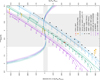 |
Fig. 3 Mass–radius relationships (left axis) computed with the DROP code in the single layer case, for iron (purple), perovskite (green), and water (cyan), and for three flattening parameters, f ∈> {0,0.1,0.2}. Values of the input parameter A are indicated along the curves for f = 0, as described in Eq. (8). The domain where the fits are performed is indicated (grey-shaded zone) as well as the absolute error (right axis). The result obtained with ρs = 1 g/cm3, f = 0 and A = 0.6 for water in Eq. (4) is shown for comparison (cyan open circle). Also plotted are the empirical relationship valid in the range 1-8 M⊕ and built from the Earth’s model by Zeng et al. (2016) (black crosses), the data from Table B.1 of Haldemann et al. (2020) obtained from the AQUA-EoS for water assuming a 300 K surface temperature (thin, dotted lines) and the results by Fortney et al. (2007) for pure-water and pure-silicate planets (open and filled squares), all obtained in the static case. See Sect. 6 for a discussion about LHS 1140 b (red dot). |
3.2 Relative changes in the mass and radius due to rotation
By differenciating Eq. (12) at f = 0, we find
 (13)
(13)
It follows that in the limit of slow rotations, the mass–radius relationship is linearly shifted upwards with respect to the static case by the quantity ∆Req = ηr f Req, where
 (14)
(14)
which depends on the mass. In the range of reference, ηr varies from 0.33 at low mass to 0.39 at high mass. For x = y = 0, we have
 (15)
(15)
which values are close to  (see Sect. I). We can see from Table D.1 that c01 is the largest among the ci1’s, whatever the material. In addition to, c11 being positive, ηr slightly increases as the mass increases.
We can make a similar analysis at constant radius. From Eq. (13), the change in the mass is ∆M = ηmfM in the limit of slow rotations, with
 (16)
(16)
which depends on the mass. The mass–radius relationship is therefore shifted leftwards with respect to the static case. We see from Table D.1 that c11 and c21 are positive, while c20 is always negative. It means that ηm < 0 monotonically decreases with the mass (it varies from -1 at to about -1.5). For x = y = 0, we get
 (17)
(17)
3.3 Inverse formula and error bars
We can determine f as a function of M and Req from Eq. (12). If we define  , then y = μ0 + μ1 f + μ2 f2, which is easily solved for f. The root is
![Mathematical equation: f=\frac{1}{2\mu_2}\left[-\mu_1+\sqrt{\mu_1^2+4\mu_2(y-\mu_0)} \right],](/articles/aa/full_html/2025/09/aa54116-25/aa54116-25-eq37.png) (18)
(18)
which becomes f ≈ (y - μ0)/μ1 for f → 0. This is therefore the flattening required to match a given mass and radius (see Sects. 5.1 and 7.1). Any uncertainty δReq in the radius (or δM in the mass) produces an error δf in the flattening, which is also the meaning of ηr and ηm (see below).
3.4 Central pressure
The central pressure, Pc, is displayed in Fig. 4 in the same conditions as above, together with the classical estimate for spherical stars (Cox & Giuli 1968) as
 (19)
(19)
which quantity is, in fact, a lower limit. We first notice the remarkable correlation between Pc and P0 in the static case, which both increase with the mass. This is expected because  , where the power-law exponent of the mass-radius relationship is, as seen before, less than
  . For a given total mass, Pc is slightly larger in the static case than for a rotating configurations. This result, which refers to a two-layer planet with modified EoS, is therefore similar with the case of a (singlelayer) polytropic gas sphere, as established in Chandrasekhar (1933a).
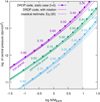 |
Fig. 4 Central pressure, Pc, in the same conditions as for Fig. 3 for f ∈ {0,0.1,0.2} and the classical estimate P0 for spherical systems (dashed line) according to Eq. (19). |
3.5 Rotation period
The rotation period, T, of the planet is displayed versus the mass in Fig. 5 for f = 0.1. As expected, T increases as f decreases, and is larger for smaller masses. A reliable fit can be obtained with the help of Maclaurin’s formula for homogeneous spheroids, which gives the rotation rate Ω as function of the mean-mass density,  and flattening, f. In the limit of slow rotations, the period of the Maclaurin spheroid
  is given by (e.g. Chandrasekhar 1933a)
 (20)
(20)
This formula works remarkably well with the modified EoS once the mean-mass density is known, as Fig. 5 shows, and the scaling with f is reliable. By expliciting the mean mass density, we can see that the quantity  should roughly be a constant (of the order of 0.3 in the present case). A quadratic fit in x and a linear fit in f appears sufficient, as follows
 (21)
(21)
where the coeficients tij are given on Appendix E. The quality of the fit is visible in Fig. 5.
3.6 Note on the very-high-mass part of the diagram
At very high mass, the radius goes through a maximum and then decreases with the mass. This behavior is the consequence of the bimodal EoS used here and is fully expected (Zapolsky & Salpeter 1969; Spiegel et al. 2014). Actually, according to the theory of polytropic spheres, the mass M and radius Req are linked as follows (e.g. Horedt 2004)
 (22)
(22)
and we have  , with the consequence that the radius remains a decreasing function of the mass (i.e. β < 0) as soon as n > 1, which is effective at very high pressure; see Table 1. The maximum occurs at about 550 M⊕ for iron and silicate and much beyond for water. It is therefore not visible in the figure, and out of the range of interest here.
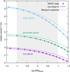 |
Fig. 5 Rotation period, T, of single-layer planets in the same conditions as for Fig. 3 for f = 0.1, together with the fit with Eq. (21). The period of the Maclaurin spheroid (dotted lines) having with the same flattening and same mean mass density according to Eq. (20) is also given. |
4 Results for two-layer planets
We ran the code with L = 2 for the same parameters A and f as above, and with q ∈ {0.1,0.2,..., 0.9}. The mass-radius relationships obtained for CE=IW in the static case are displayed in Fig. 6 as a function of q for a given A (hereafter, a q-sequence), and as a function of A for a given q (hereafter, a A-sequence). A sub-figure shows the effect of rotation for f = 0.2. The data obtained for f = 0.1 and q = 0.5, which corresponds to Saturn’s oblateness, are gathered in Table A.1 (bottom). We see that the mass–radius relationship stands between the two curves obtained in the single-layer cases C={I,W} and we have similar trends as for single-layer cases (i.e. the radius increases as f increases). The A-sequences are roughly linear in the domain of interest, parallel to each other, but with a marked curvature at high mass. All q-sequences are also roughly parallel to each other but are non-bijective, for any A. As q increases, the mass and radius first decrease until q ≈ 0.6, then the variation is fully reversed. The results obtained for iron/perovskite and for perovskite/water are displayed in Figs. F.1 and G.1, respectively. We make similar observations as for the IW planet. The diagrams are a little bit more compact because ρs(C)/ρs(E) is smaller than for the IW case.
4.1 Fitting procedure
Whatever the mineralogical composition, we can fit the data in the reference mass range (see Sect. 3) by a quadratic law, namely, with Eq. (10). The process is a little bit more complex than for the single-layer case, because there is an additional parameter. The coefficients obtained for each A-sequence where q and f are held fixed are henceforth denoted as c′i, with i = {0,1,2}. These are listed in Table H.1 for the static IW planet, together with mean values  and half-amplitudes of variation ∆i defined by
 (23)
(23)
where the single-layer data are excluded. This procedure is repeated for each value of the flattening parameter.
4.1.1 A sigmoid for the coefficient c′0
We find that c′0 exhibits marked variations with the core size. It is plotted versus q in the IW case in Fig. 7 for all the flattening parameters considered, including the static case. In fact, c′0(q) can be approximated by a smooth function, but a quadratic law is not really appropriate. A better choice is a symmetrical sigmoid, namely,
 (24)
(24)
where the coefficient d0 = y(0) corresponds in principle to the single layer case; see the coefficients c0j in Tables C.1–C.3. The analysis reveals that d0, d1, d2 and the exponent σ vary very weakly with f, and can all be fitted by a parabola. However, for Eq. (24) to be easily/analytically reversible in the variable f, we deliberately use a unique value for σ regardless of the flattening parameter, f. We then decide to use the value obtained in the static case, namely σ ≈ +2.7. The parameters d0, d1 and d2 of the sigmoidal fit are given in Table H.2 for the IW planet. It happens that these quantities vary monotonically with f, and can be very well approximated by a parabola, again, i.e.  . The coefficients dij of these three fits are listed in Table I.1 for CE={IW,IP,PW}. Figure 7 also displays the absolute error in fitting c′0 by Eq. (24), which turns out to be less than about 0.001 for q ≤ 0.9 and f ≤ 0.2. We get a similar magnitude for the IP and PW cases.
4.1.2 A parabola for the next two, averaged coefficients
Figure I.1 shows the mean values 〈c′1〉 and 〈c′2〉 and the associated deviations ∆i defined by Eq. (23) versus f, still in the IW case. We see that, in contrast with c′0, the coefficients c′1 and c′2 do not vary much with the core size q. The size of the error bars is about 0.002 at most for c′1 and about 0.003 for c′2, in absolute. As c′2 is lower than c′1 by a factor 10 for any f ≤ 0.2, working with mean values introduces an absolute error in y of the order of 0.002, mainly caused by the substitution  . As |x| ≤ 1 for the reference mass range, the impact is an error of the order of 0.002 in y. Next, we use a parabola to fit
  , namely,
 (25)
(25)
while a linear function appears sufficient for 〈c′2〉. The coefficients c′1j and c′2j are listed in Table I.1 of the Appendix for the three types of composition. The quality of these two fits is visible in Fig. I.1 (right axis) for CE=IW. As the absolute error is less than 10-4, the error is dominated by the averaging procedure, i.e. 0.002 in absolute, and not by the fit of mean coefficients.
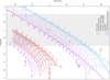 |
Fig. 6 Same caption as for Fig. 3, but in a two-layer IW planet, in the static case. Labels refer to values of top-to-bottom mass density ratio A (single-layer) and the relative size of the core q along the sequences. The effect of rotation is also shown for f = 0.2 (bottom right, red lines; a vertical shift of -0.6 applied for clarity). |
4.2 The parametric mass–radius relationship
It follows that we get a complete parameteric expression of the mass–radius relationship for two-layer planets, namely,
 (26)
(26)
The fractional size of the core, q, is uniquely contained in the first term, while the effect of rotation is hidden in all the coefficients. Given the discussion above, the absolute error in fitting y is estimated to
 (27)
(27)
which corresponds, at most, to a relative error of 1.5% in the radius for the whole reference mass range. Depending on the application and context, Eq. (26) can be adapted or degraded, for instance by omitting quadratic terms in x and/or f. The advantage of this formula is that it is easily inversible in any of the two variables M and q (see below). We can test Eq. (26), for instance in the IP case, by setting M = 1 M⊕ (i.e. x = 0), q = 0.5 and f = 0.05, which corresponds to the example of Fig. 2. The formula gives y ≈ -0.00196, leading to Req ≈ 0.99551 R⊕. This is in excellent agreement with the value determined by the DROP code and reported in Table 2.
4.3 Effect of rotation detailed
As done for the single-layer case, we can differentiate Eq. (26) in the vicinity of f = 0. The partial derivatives are
 (28)
(28)
and
![Mathematical equation: \begin{flalign} \nonumber \left.\frac{\partial y}{\partial f}\right|_{q,f} \approx & \left[\frac{d_{01}+d_{11}q^\sigma }{1+d_{20}q^\sigma}-\frac{(d_{00}+d_{10}q^\sigma)d_{21}q^\sigma }{(1+d_{20}q^\sigma)^2}\right]\\ & +c_{11}'x+ c_{21}'x^2,\end{flalign}](/articles/aa/full_html/2025/09/aa54116-25/aa54116-25-eq58.png) (29)
(29)
and these depend on the mass and especially on the fractional size. We note that the power-law index, β, of the mass–radius relationship is given by 〈c′1〉, which is mainly represented by the coefficient c′10. This coefficient is close to 0.3, as in the single-layer case. We can then deduce ηr by varying the radius at constant mass, and ηm by varying the mass at constant radius, namely,
 (30)
(30)
and
 (31)
(31)
Figure 8 shows the ηr and ηm versus q for the three types of compositions. We notice that response to rotation goes through an extremum, which is fully calculable from Eq. (29). In the static case, the extremum stands at q ≈ 0.62 for an IW planet, which corresponds to a core mass fraction of 0.65 from Fig. 9. This is q ≈ 0.73 and M1/M ≈ 0.60 for the IP planet, and q ≈ 0.67, and M1/M ≈ 0.56 for the PW planet.
We can continue this analysis by considering the third derivative, ∂y/∂q, and define
 (32)
(32)
which gives the link between f and q keeping simultaneously the mass and the radius of the planet fixed. For instance, a PW configuration with f = 0 and q = 0.5 has the same mass and same radius as another PW confguration with f = 0.1 and q = 0.5 + 0.1 × 1.16 ≈ 0.616 (since we get ηq ≈ 1.16 from the graph). This formula must, however, be manipulated with caution because f is intended to be much smaller than unity as well as ∆q. Figure 8 shows ηq versus q. As expected from Figs. 6, F.1 and G.1, the changes are relatively small for core sizes larger than about 0.6, and very large at small q.
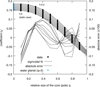 |
Fig. 7 Coefficient c′0 obtained in the IW case fitting the mass-radius relationship for a given value of the core fractional size, q, for each flattening parameter, f (dots). The fits by a sigmoid are superimposed (plain lines), and the absolute error is also shown (dashes lines, right axis). |
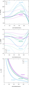 |
Fig. 8 Parameters ηr (top), ηm (bottom) and ηq (bottom) measuring the relative change in the equatorial radius, mass and core fraction respectively with rotation (in units of f) as a function of the core size q for 0.1 Me, 1 Me, and 10Me. |
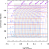 |
Fig. 9 Core mass-fraction versus the mass for the IW planet in the static case (colour gradient) and for f = 0.2 (red). See Appendix J for the IP and PW planets. |
4.4 Core and envelope discrimination
Following the fitting procedure, q appears only in the sigmoidal representation of coefficient c′0. As a consequence, we can express the relative size of the core as function of the mass, radius and flattening parameter. From Eq. (26), we find
![Mathematical equation: \begin{flalign} \qpol = \left[\frac{y - c_1' x -c_2'x^2-d_0}{d_1-d_2\left(y - c_1' x -c_2'x^2\right)} \right]^{\frac{1}{\sigma}} \equiv q(x,y,f),\end{flalign}](/articles/aa/full_html/2025/09/aa54116-25/aa54116-25-eq62.png) (33)
(33)
which assumes that the term inside the brackets is positive (and less than unity). It is of particular interest because it gives a first estimate of the relative size of the core for a given mass and radius (Brinkman et al. 2024). This avoids a full scan of the parameter space. We note that any uncertainty in the radius and/or mass induces an error, δq, in the fractional core size, q (see Sect. 5).
mass=1.;dmass=0.1;radius=1.3;dradius=0.13 mass=1;dmass=0.1;radius=0.85;dradius=0.085
4.5 Core mass fraction and rotation period
The core mass-fraction M1/M is unfortunately not an input in the simulations, but an output. It is shown in Fig. 9 for the IW configurations, and for f ∈ {0,0.2}; the figures obtained in the IP and PW cases are reported in the Appendix J. We see that the core mass-fraction is very well correlated with the core size, q. This is true whatever the rotation state of the planet. The effect of rotation is weak. For a given total mass and fractional size of the core q, the core mass-fraction is the largest when the planet is static, and it decreases with rotation. Figure 10 shows the rotation period, T, versus the mass for f = 0.1. As for the single-layer case, the scaling with f given by Eq. (20) is reliable. The rotation period decreases with increasing mass, which is the consequence of the rise of the mean mass density  with M. As we have Req(IW) > Req(IP)Req(PW) for a given mass, T is the largest for IW planet, and the lowest in the PW case.
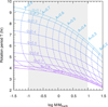 |
Fig. 10 Same caption as for Fig. 9, but for the period T computed for f = 0.1; see Appendix J for the IP and PW planets. |
5 Error bars
Positioning a planet in pre-computed mass–radius relationships for single layers enables us to determine how close or far the body is to a pure composition. Therefore, it allows us to deduce plausible combinations of compositions, either in the form of a mixture of materials or in the form of distinct layers (see below). In terms of number of layers, composition and rotational state, the level of degeneracy depends not only in the position but also on the size of error bars on the radius, δReq, and on the mass, δM.
5.1 Single-layer models
As shown in Sect. 3, including rotation moves the mass–radius relationship upwards (i.e. towards larger radii). Thus, if observational error bars permit, a position in the diagram can be interpreted in terms of a deviation to a pure composition or in terms of rotation, or both. This can easily be checked by running the DROP code by selecting all values of f that lead to a given pair (M ± δM, Req ± δReq), but a scan of the parameter space is costly. The advantage of the simulation is that we can impose high values of f, up to the break-up velocity. In the theory of ellipsoidal figures of equilibrium Chandrasekhar (1969), the homogeneous spheroids in rigid rotation are stable for values of the flattening parameter up to f ≃ 0.42, which corresponds to the transition towards states of lower energies in the form of triaxial bodies. However, if f ≤ 0.2, we can use Eq. (18) as an approximation, and we can include the corresponding error bars δx and δy, and even use the ηm and ηr parameters for small f values. An illustration is given in Sect. 6.
5.2 Two-layer models
With two-layer diagrams, the degeneracy increases and the interpretation is less clear. For instance, we see from Figs. 6, F.1 and G.1 that the data (x,y) = (1,0.3) is compatible with static IW, IP and PW planets, differing by the size of their core. Again, in the spherical case, we can scan the region in the diagram numerically with the DROP and select the right pairs (q, A) on input compatible with error bars. We then get a range δq of fractional sizes as the image of (x0 ± δReq, y0 ± δM). As shown, rotation represents another degree of freedom (and a source of confusion in the inverse problem). We can therefore repeat this treatment by varying f, and it follows that δq becomes a function of f . In fact, we can directly access the image of error bars in terms of q and f by using Eq. (33).
As an illustration, we show in Fig. 11 two positions (x0 ± δx, y0 ± δy) in the IW diagram, and the image of error bars in terms of core size, q, obtained from Eq. (33) in the static case of f = 0 and for f = 0.2. The extreme points Ci obtained by considering ±δx and ±δy are also reported. We see that:
the image of the error bar in the radius, Req ± δReq, is an error bar in the core size around q0,
the image of the error bar in the mass, M ± δM, is another error bar in the core size around q0,
the two error bars in the core size are not equal, not symmetrical around q0, non-linear in δReq and δM, and sensitive to rotation.
Error bars in terms of fractional size. We see from the figures that q ∈ [qmin, qmax], where the lower and upper bounds correspond to points C2(x0 - δx, y0 + δy) and C4(x0 + δx, y0 - δy), respectively. We can therefore retain
 (34)
(34)
where δx > 0 and δy > 0. We note that qmin and qmax are not symmetrical with respect to q0 = q(x0, y0, f), unles the uncertainties are small. In these conditions, we have
 (35)
(35)
in the general case. In the limit of small uncertainties, we can deduce an expression for δq by differenciation of Eq. (33). This approach uses the derivatives established in Sect. 4.3.
Error bars in terms of flattening. The flattening parameters compatible with a given observational data can be estimated from ηr and ηm, by using Eqs. (30) and (31) where ∆Req and ∆M are to be replaced by δReq and δM, respectively. Assuming that the spherical configuration f = 0 is reachable by the model and q is fixed, we have
 (36)
(36)
which differs from one composition to another. So, for a given fractional size q, we have
 (37)
(37)
where δf can be directly read from Fig. 8.
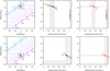 |
Fig. 11 Four sets of fiducial data (M ± δM, Req ± δReq) placed in the mass-radius relationship for IW planets (left panels) for M = 1M⊕, and Req = 1.3 R⊕ (top) and Req = 0.85 R⊕ (bottom). Error bars are δM/M = 0.1 and δReq/Req = 0.02 (black, plain lines) and δM/M = 0.02 and δReq/Req = 0.1 (black, dotted lines). The image of the error bars in terms of fractional size q is shown in the static case (middle panels) and with fast rotation f = 0.2 (right panels). See also Fig. 6. |
6 Illustration with the parameters of LHS 1140 b
For a suitable application, we searched for a transiting superEarth with a confirmed status and a good precision on the mass and on the radius. We have selected the targets from the Nasa Exoplanet Archive (Akeson et al. 2013) and European exoplanet database with a maximum radius of 1.8 R⊕. From the semi-major axis a and mass M⋆ of the host star, the candidates have then been ordered with increasing parameter  which scales with their tidal locking time (Zahn 1989; Leconte et al. 2015; Barnes 2017). Unfortunately, all robust super-Earth candidates with a radius measurement currently discovered are expected tidally locked, because of their short orbital periods and presumed age. The comparison with our models can therefore not account for the final spin state of the planet, and therefore remains purely illustrative. We have selected LHS 1140 b, which represents a fair trade off, because it exhibits among the largest synchronisation time scale. This planet has been detected by both photometric transit and radial-velocity measurements by different groups (Dittmann et al. 2017; Ment et al. 2019; Lillo-Box et al. 2020; Cadieux et al. 2024a). It orbits a M-dwarf star located at about 12 pc away from the Sun. It has an averaged mass-density compatible with an iron and/or silicate content. In addition, the installation conditions seem to permit water, if present, to be in liquid phase, making this object of particular interest in several respects (Wandel 2018). This planet has recently been modelled by Rigby & Madhusudhan (2024) and Daspute et al. (2024), with up to four differentiated layers (including a thin atmosphere). The water layer could be 2000 km deep, and the ocean might represent up to 7% of it in the nominal cases. The internal structure of LHS 1140 b is still under debate. It is commonly interpreted as either a water world or a miniNeptune, but the recent spectroscopic observation with JWST disfavours a body with dihydrogen- and methane-rich atmosphere; hence, we highlight the second option (Cadieux et al. 2024b).
In this section, we use Rsph = 1.730 ± 0.025 R⊕ as the spherical radius and the mass is M = 5.60 ± 0.19 M⊕, according to Cadieux et al. (2024a). In decimal logarithm, these data correspond to  and
and  . In the absence of any information about the orientation of the rotation axis with respect to the line of sight, we assume Rsph = Req for simplicity. This setting is correct only in the case of a circular transit, i.e. the planet is exceptionally seen pole-on. We can then directly place the planet in the mass–radius diagrams, without any bias. Otherwise, a correction must be applied (see Sect. 7.4).
6.1 Single-layer models
We see from Fig. 3 that a pure water planet is not possible, and that the iron hypothesis is not sustainable, unless a very large rotation rate is invoked. Actually, as shown before, the mass– radius relationships are shifted upwards when f > 0, and the faster the rotation, the larger the shift. The only plausible solution is obtained with perovskite, but some rotation is necessary. According to the figure, f < 0.1 at a one sigma confidence level. A zoom is presented in Fig. 12. By using the DROP code, we find f = 0.055 for the central value of the observational interval, while we get f ≈ 0.064 from the fit by Eq. (18). The deviation between these two values is due to the quality of the fit. By considering errors bars and especially points C2 and C4 (see Sect. 5), we get the values of Table 3, where the associated rotation period is also reported.
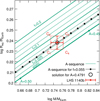 |
Fig. 12 Position of LHS 1140 b (red) in the mass–radius diagrams for single-layer, pure-perovskite planets obtained for different flattening parameters. The A-sequence obtained with the DROP code for f = 0.055 is also plotted (black); see Fig. 3. |
6.2 Two-layer models
Figure 13 shows the position of the planet in the mass–radius diagrams for an IW, an IP and a PW planet, together with the error bars through the points Ci ’s. We can feed Eq. (26) with the observational data, and in particular with the error bars, as done in the single-layer case. The results obtained for three rotational states are gathered in Table 4. In the static case, LHS 1140 b is compatible with an iron core/water envelope planet for q ≈ 0.64 ± 0.03, and with a perovskite core/water envelope planet for q ≈ 0.94 ± 0.04, while the IP solution is ruled out. New solutions are permitted with rotation. While we can consider relatively large values for f, it is interesting to use Eq. (36) to get the range of rotation states compatible with the error bars. For LHS 1140 b, we have δRsph/Rsph ≈ 0.01445, and δM/M ≈ 0.03393. As a consequence, from the fractional size obtained in the spherical case, for the range of flattening parameters compatible with the error bars, we find
δf ≈ 0.029 for the IW planet,
δf ≈ 0.038 for the PW planet,
and the corresponding period is T ≈ 7.5 h in both cases.
The IW hypothesis. If rotation is accounted for, type IW solutions remains fully available. The iron core is larger and more massive. By using the DROP code, we can scan the parameter space and extract the structures compatible with the observational data. In this task, Eq. (33) is of great help as the right range of fractional sizes is fastly identified. Figure 14 shows the fractional size, q, the parameter A, the core mass fraction, M1/M, the central pressure, Pc, an estimate of the ocean depth (see Sect. 7.3) and the rotation period, T, obtained for f ∈ {0,0.1,0.2}. We see that the range of fractional sizes as given by Eq. (33) is in very good agreement with the numerical approach. We find q ≈ 0.635 ± 0.025, and the core-mass fraction is 0.66 ± 0.04 in the non-rotating case. These ranges are pushed towards higher values with rotation. The ocean-depth is estimated to be at least about 30 km, and it decreases as f increases. The rotation period, which roughly varies like 1 / √f, is already as low as about 4 h for f = 0.1.
The IP hypothesis. As Table 4 shows, an iron core/perovskite envelope planet is a plausible option for LHS 1140 b, but this requires some rotation, again. The core has a small size and a low mass in relative. For f = 0.1 for instance, we have  . We have plotted in Fig. 13 (middle panel) the A-sequence obtained with the DROP code for f = 0.05 and q = 0.15. The solution obtained for A ≈ 0.4866 matches the central value (x0, y0) very well. Output data are gathered in Table 5 and the pressure and mass-density maps are displayed in Fig. 15. In this simulation, the iron core is less than 1% of the planet’s mass, the rotation period is 6 h 24 min.
The PW hypothesis. This solution is relatively constrained in the sense that it persists only if f is very small according to Fig. 13 and Table 4. As quoted above, f ≤ δf ≃ 0038. It means that LHS 1140 b can be a huge, slowly rotating silicate body with a shallow water envelope.
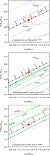 |
Fig. 13 Position of LHS 1140 b (red) in the mass–radius diagram for IW planets (top), for IP planets (middle) and for PW planets (bottom). The one-sigma error bars are taken from (Cadieux et al. 2024a). The best static A-sequence is also plotted for IW and PW configurations (black). See also Fig. 15 and Table 5. |
6.3 Discussion
The results presented above are in good agreement with the ternary diagrams presented in the spherical case in Daspute et al. (2024), based in the 1D computational code by Zeng & Seager (2008) with updated EoS. In fact, these authors did not rule out a two-layer structure for this planet, and the core mass-fractions predicted for the IW and PW configurations are similar to those reported in this work.
Although the IW configuration is not really realistic, the large f -values presented in Fig. 14 better illustrate the additional degeneracies for the internal structure of such terrestrial planets when rotation is accounted for. For LHS 1140 b, they correspond to very small rotation periods of a few hours only (close to the critical angular velocity), which must be regarded as illustrative cases and cannot represent the genuine, current spin rate of LHS 1140 b. Indeed, this planet orbits at a short stellocentric distance (<0.1 au), where the tidal locking time is expected to be much shorter than the system age of 5 Gyr. Its initial rotation must therefore have converged towards an equilibrium state between gravitational and thermal atmospheric tides, if any atmosphere is present (e.g. Leconte et al. 2015). Actually, for each composition of our double-layer model, we can estimate the maximum (‘primordial’) value of f compatible with the observational error bars (for instance, f ≈ 0.029 corresponds to a minimum period T ≃ 7.5 h for the IW case, see Fig. 14).
High spin rates are nevertheless not excluded for young, solid planets. In the current paradigm, giant impacts are expected to play a significant role at late stages of the planet formation process, and can spin-up planets close to their breakup velocity (e.g. Kokubo & Ida 2007; Miguel & Brunini 2010). In their recent collision scenario for the Earth-Moon system, to form the Moon from the Earth’s mantle, $Cuk & Stewart (2012) even invoked a pre-impact spin rate of 2.3 h only for the proto-Earth. Pebble accretion is also thought to offer a valuable mechanism to significantly spin-up solid protoplanets through angular momentum transfer from the pebbles flow to the surface of the forming planet (Johansen & Lacerda 2010; Visser et al. 2020). Pebble accretion might be able to yield such fast (initial) rotation periods close to the critical break-up value for terrestrial planets (Takaoka et al. 2023), although recent developments suggest that the final outcome for the planetary spin strongly depends on the details of the modeling of the angular momentum transfer through the planet’s primordial atmosphere (Yzer et al. 2023). Due to a methodology bias and sensitivity limitation of the transit technique, studying spin distributions and constraining planetary oblateness remains limited to the gaseous giants, as no genuine super-Earth has been detected by the transit technique beyond the tidal locking region so far; see e.g. Liu et al. (2025) for Kepler167e, and Lammers & Winn (2024) for Kepler51d. Within the next decade, the PLATO mission (Rauer et al. 2024) is expected to populate this domain with dozens of Earth-like and Super-Earth planets with orbital periods long enough (≳100–200 d) to escape tidal braking.
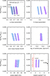 |
Fig. 14 Structure parameters of LHS 1140 b compatible with the error bars (see Fig. 13, top panel) computed with the DROP code, assuming a two-layer, IW planet in three rotational states. The colour code refers to values of the core fractional size, which is smaller in the static case than with rotation; see also Fig. 6. Regarding the ocean depth, see Sect. 7.3. As an indication of the break-up velocity (which depends on q), we have reported in the last panel the Keplerian period at the planet equator (red) as well as the period associated with δf = 0.029, which amplitude corresponds to the error bars in the static case; see Eq. (36). |
 |
Fig. 15 Same caption as in Fig. 2 but for LHS 1140 b, assuming a rotating IP planet with q = 0.15 and f = 0.05. See also Table 5 and Fig. 13 (middle panel). |
7 Summary, discussion, and perspectives
7.1 Mass-radius-flattening relationships (summary)
In this work, we compute mass–radius relationships for singlelayer and two-layer planets, including solid-body rotation by a conservative approach, leading to ‘mass–radius–flattening’ relationships. We selected three types of materials composing the core and the envelope, namely iron, perovskite, and water, along with the bimodal EoS from Seager et al. (2007). The data tables are available in electronic form (see note 2). We refer to Appendix A for a sample. Any specific simulations can be performed upon request.
In the reference mass-range from 0.1 to 10 M⊕, the mass– radius relationships (log. values) are aptly fitted by a quadratic law when rotation is accounted for. Despite the fact that the fits are valid over only two decades in terms of mass, these are fully reversible in any of the three parameters M, q, and f. This is very useful to get rapid insight of permitted configurations, in terms of core size and rotational states. For single-layer planets, we can summarise the results as follows:
the mass–radius relationships are given by Eq. (12) where the nine coefficients, cij, can found in Table D.1;
the inverse formula f (M, Req) is given by Eq. (18);
-
in the static case, we have
 (38)
(38)where the upper (lower) value refers to the lower (resp. upper) bound in the mass reference range,
the relative change in the radius (at constant mass) and in the mass (at constant radius) due to rotation are ηrf and ηm f, respectively, as expressed in Eqs. (14) and (16);
the rotation period is available from Eq. (21), where the coefficients are listed in Table E.1;
for a given mass, the central pressure is slightly decreased, which meets the result established in the single-layer, polytropic case by Chandrasekhar (1933a).
For two-layer planets, the core fractional size, q, is the additional parameter. The mass–radius–flattening relationships can still be fitted in this case, with a sigmoid for q. It follows that:
the mass–radius relationships are described by Eq. (26), where the coefficients ci′j, dij, and σ are given in Table I.1;
-
in the static case and for a given fractional core size, q, we have from Eq. (28) and Table I.1;
 (39)
(39)where the upper (lower) value refers to the lower (resp. upper) bound in the mass reference range;
the relative change in the radius (at constant mass) and in the mass (at constant radius) due to rotation are found from ηr f and ηm f, respectively. This is expressed in Eqs. (30) and (31) and Fig. 8;
for a given mass, radius, and the associated uncertainties (x0 ± δx, y0 ± δy), the relative size of the core (and uncertainty) can be determined from Eq. (33), and it depends on rotation. This is shown, for instance, in Fig. 11);
in the limit of small flattenings, f, can be expressed as a function of M, Req, and q.
The numerical survey reveals that the relative change in the radius (mass) at constant mass (radius respectively) due to planet spin (see Sect. I), which is measured by the parameter ηr f (ηm f, respectively) is significantly larger than for a rotating, homogeneous body. This is marginally significant for single-layer planet, but more pronounced for two-layer planets with core size of q ≃ 0.70 ± 0.05 depending on the composition, as shown in Fig. 8.
7.2 Slope and ‘effective’ polytropic index
As a direct consequence of the EoS, the power-law exponent is β ≈ 0.3 for single and two-layer planets, for the mass range of reference. This is slightly larger than the result reported in Seager et al. (2007), who considered a wider range of reference, and in Boujibar et al. (2020). It is also more compatible with values extracted from exoplanet catalogs (Parc et al. 2024). This result remains in good agreement with Fortney et al. (2007), both in terms of absolute position and slopes (slightly larger here), despite slight differences in the EoS (in particular ρs). We have seen that β depends on f, via the coefficient c1 and 〈c′1 〉, and is larger with rotation. It would therefore be very interesting to understand the individual role or effect of the three parameters ρs, A (i.e. K), and m in these laws, and more generally, to determine how the coefficients in the fits depend on these three parameters. In the static case, this can be performed directly from the Lane-Emden equation.
According to Eq. (22), a power-law of the form R ∝ Mβ corresponds to a single-layer polytropic EoS with index
 (40)
(40)
As β ≈ 0.3 in all cases presented in the article, the bimodal EoS corresponds to an ‘effective’ polytropic index  . Values of neff obtained for the single-layer and two-layer planet examined in the article are listed in Table 6. It means that the mass–radius relationships computed from Eq. (4) can be reproduced with a single layer polytrope with index neff. The fact that neff remains close to 0 means that the global internal structure is close to a piling of homogeneous layers, as mass density profiles show.
7.3 Note on the ocean depth of water-rich planets
When the outer layer is made of water, and the conditions are met at the surface for water to be in liquid phase, then we can determine the depth, d, of the liquid ocean by considering the pressure and density at which the phase transition to high pressure iceice VII occurs. This point in principle depends on temperature. As a typical/low value (Léger et al. 2004), we can take 1010 dyn/cm2 ≡ Pref and solve P(R, Z) = Pref numerically for any structure computed with the DROP code. In contrast to the spherical case, d is expected to depend on the latitude. We can give an estimate of the ocean depth at the pole from the equation of hydrostatic equilibrium, namely,
 (41)
(41)
and the impact of rotation. In the limit of small flattening values f → 0, we have for any homogenous spheroid (e.g. Binney & Tremaine 1987)
![Mathematical equation: \Psi(0,Z) \approx - \frac{2}{3}\pi G \rho \left[(3-2f) \req^2 - \left(1+ \frac{4}{5}f \right) Z^2 \right],](/articles/aa/full_html/2025/09/aa54116-25/aa54116-25-eq82.png) (42)
(42)
Assuming d2 ≪ Rpol2 and that the effect of rotation on the gravitational acceleration in the surface layer is not greatly altered by spheroidal stratification with respect to the Maclaurin spheroid, we have Pref ≈ ρsg[Ψ(Rpol) - Ψ(Rpol - d)]. So, we find from Eq. (41)
 (43)
(43)
and it follows that d decreases with the mass (we have d ∝ M2β-1), and decreases as rotation increases. By setting Pref ≈ 1010 dyn/cm2, we get
 (44)
(44)
which is for a non-rotating planet with same size and mass as the Earth (note that this value is obviously sensitive to ρs, and we would get a 30% larger depth for ρs = 1 g/cm3). In the general case, we find
 (45)
(45)
and we can use Eq. (10) or Eq. (26) to get a function of x, q, and f only. We note that the impact of rotation, which is weak, is not only supported by the term  f, but also by y which depends on f too. For LHS 1140 b, the ocean depth estimated from the DROP code is about 33 km in the static IW case (see Fig. 14), while Eq. (45) predicts 37 km. We verified that the depth at the equator is a little bit larger than at the pole, which is the consequence of the mass-density gradient, which is slightly weaker along the equatorial axis.
 |
Fig. 16 Two extreme orientations of the rotation axis of the planet with respect to the line of sight (perpendicular to the figure) during a transit, relative to the spherical case. |
7.4 Corrections in the mass–radius relationships due to the planet oblateness and axis orientation
When the radius is deduced from transit method, the planet is generally assumed spherical, meaning that the obstacle to the star light seen by the observer is a circular disc. This case is slightly different if the planet is spinning. Following Berardo & de Wit (2022), two extreme geometries of the primary eclipse can be considered, as sketched in Fig. 16:
during a circular transit, the rotation axis is always oriented towards the observer (case b), then the blocking section is a disc and the area is
 ;
;during an oblate transit, the rotation axis is always perpendicular to the line of sight (case c), then the relevant shape is roughly an elliptic disc, and the area is
 .
.
Regarding photometric signals, there is no difference between a spherical planet (case a) and a pole-on, spinning planet (case b). In the latter situation, however, the position of the planet in the mass–radius relationship is higher than it would be in the static case, leaving the impression that the planet contains a larger fraction of light compounds. For an oblate-transit (case c), we have  , which leads to
 (46)
(46)
with the same notation as for Eq. (26). In this case, without sufficient resolution to detect the rotation state at the ingress and egress of the transit, then the position of the planet in the mass– radius relationship based upon Rsph leaves the impression that the planet contains heavier elements, because it is in fact higher in the diagram. We see that the correction for an oblate transit in the mass–radius relationships can be accounted self-consistently for by inserting Eq. (46) into Eq. (33). Thus, we find
![Mathematical equation: \begin{flalign} \qpol = \left\{\frac{\ysph - \frac{1}{2} \tau \log(1-f) - c_1' x -c_2'x^2-d_0}{d_1-d_2\left[\ysph - \frac{1}{2} \tau \log(1-f) - c_1' x -c_2'x^2\right]} \right\}^{\frac{1}{\sigma}},\end{flalign}](/articles/aa/full_html/2025/09/aa54116-25/aa54116-25-eq97.png) (47)
(47)
where we have introduced the parameter τ ∈ [0, 1] (i.e. it is zero for a circular transit and unity for an oblate transit).
For LHS 1140 b, an oblate transit means a larger equatorial radius. With f = 0.05 as considered in the figures, the ‘true’ equatorial radius becomes Req ≈ 1.77.
We show in Fig. 17 the effective position of LHS 1140 b in the PW diagram with flattening of f = 0.05, assuming an oblate transit, together with the A-sequence that crosses the new effective central value, namely,  . In this case, the ‘true’ equatorial radius becomes Req ≈ 1.77. Figure 18 displays the structure corresponding to this new point, and Table 7 lists the new data for this equilibrium.
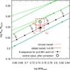 |
Fig. 17 Effective position of LHS 1140 b in the PW diagram if the rotation axis of the planet is perpendicular to the line-of sight, corresponding to an oblate transit for f = 0.05. See also Figs. 13 (bottom) and 16. |
7.5 Three layers and more
A natural continuation of this work is the introduction of new layers. A three-layer rotating planet made of an iron core, a silicate intermediate layer (mantle) and a water envelope, namely, an IPW planet, would be of particular interest for LHS 1140 b, as it is located very close to a pure perovskite composition, as reported in Valencia et al. (2007a). According to our analysis, the internal structure of LHS 1140 b is compatible with i) a small iron core surrounded by a large silicate mantle and ii) a thin water surface layer on top of a big silicate core, as depicted in Figs. 15 and 18. Thus, it would be interesting to consider a mixture of these two extreme configurations, in the form of a three-layer body. As explained in Daspute et al. (2024), the silicate mantle should not make up more than 39% of the planet in terms of size, to the advantage of the water and iron layers. This question merits indeed an extension of our approach to configurations with L = 3. Considering an additional atmosphere (e.g. made of hydrogen and helium or water vapor) and studying the response of a gas phase to rotation is another challenge to face (Adams et al. 2008).
Fitting the mass–radius relationship should become very complicated for L > 2 because the number of parameters increases. In fact, each new layer requires two new parameters (the mass-density and the relative position with respect to the others). This addresses the question of the computing time. Accounting for more layers means is costly. With the modified polytropic EoS running the DROP code is already longer, in particular, due to the special function (see Appendix B). It would be interesting to have both H(ρ) and ρ(H) available in the form of an approximation, for each index m of the EoS. A preliminary inspection shows that 1/2F1(u) can be very well fitted by a low-degree polynomial in ![Mathematical equation: $u \in [0,\frac{1}{2}]$](/articles/aa/full_html/2025/09/aa54116-25/aa54116-25-eq102.png) . With a second-order polynomial, easily reversible, the relative precision is already on the low level of a few 10-4. With such an option, some computing time is saved and this would enable us to increase the number of layers by maintaining the actual resolution. An alternative is to use the method of dimension reduction, as proposed in Staelen & Huré (2024), which is currently being examined.
. With a second-order polynomial, easily reversible, the relative precision is already on the low level of a few 10-4. With such an option, some computing time is saved and this would enable us to increase the number of layers by maintaining the actual resolution. An alternative is to use the method of dimension reduction, as proposed in Staelen & Huré (2024), which is currently being examined.
 |
Fig. 18 Same caption as for Fig. 15 but assuming a PW planet and an oblate transit with f = 0.05 (the period is T ≈ 6 h). See also Table 7 and Fig. 17. |
Acknowledgements
This research has made use of the NASA Exoplanet Archive, which is operated by the California Institute of Technology, under contract with the National Aeronautics and Space Administration under the Exoplanet Exploration Program (retrieved on Dec 13, 2024). This research has made use of data obtained from or tools provided by the portal exoplanet.eu of The Extrasolar Planets Encyclopaedia. This work was supported by the Programme National de Planétologie (PNP) of CNRS-INSU co-funded by CNES. Computer time was provided by the computing facilities MCIA (Mésocentre de Calcul Intensif Aquitain) of the Université de Bordeaux. It is a pleasure to thank M. Turbet, F. Chambat and Y. Ricard for very interesting inputs and advices on the article prior to submission, and J. Leconte. We are grateful to the referee, Dr. A. Aguichine, for his very detailed report and the many criticisms, questions and suggestions to improve the article.
References
- Adams, E. R., Seager, S., & Elkins-Tanton, L. 2008, ApJ, 673, 1160 [Google Scholar]
- Agol, E., Dorn, C., Grimm, S. L., et al. 2021, Planet. Sci. J., 2, 1 [NASA ADS] [CrossRef] [Google Scholar]
- Aguichine, A., Mousis, O., Deleuil, M., & Marcq, E. 2021, ApJ, 914, 84 [NASA ADS] [CrossRef] [Google Scholar]
- Akeson, R. L., Chen, X., Ciardi, D., et al. 2013, PASP, 125, 989 [Google Scholar]
- Akinsanmi, B., Barros, S. C. C., Santos, N. C., Oshagh, M., & Serrano, L. M. 2020, MNRAS, 497, 3484 [NASA ADS] [CrossRef] [Google Scholar]
- Amendt, P., Lanza, A., & Abramowicz, M. A. 1989, ApJ, 343, 437 [NASA ADS] [CrossRef] [Google Scholar]
- Auclair-Desrotour, P., Farhat, M., Boué, G., Deitrick, R., & Laskar, J. 2024, arXiv e-prints [arXiv:2410.16200] [Google Scholar]
- Barnes, R. 2017, Celest. Mech. Dyn. Astron., 129, 509 [Google Scholar]
- Basillais, B., & Huré, J.-M. 2021, MNRAS, 506, 3773 [NASA ADS] [CrossRef] [Google Scholar]
- Berardo, D., & de Wit, J. 2022, ApJ, 935, 178 [NASA ADS] [CrossRef] [Google Scholar]
- Binney, J., & Tremaine, S. 1987, Galactic Dynamics (Princeton, NJ: Princeton University Press), 747 [Google Scholar]
- Boujibar, A., Driscoll, P., & Fei, Y. 2020, J. Geophys. Res. (Planets), 125, e06124 [Google Scholar]
- Brinkman, C. L., Polanski, A. S., Huber, D., et al. 2024, arXiv e-prints, [arXiv:2409.08361] [Google Scholar]
- Brugger, B., Mousis, O., Deleuil, M., & Deschamps, F. 2017, ApJ, 850, 93 [NASA ADS] [CrossRef] [Google Scholar]
- Cadieux, C., Doyon, R., MacDonald, R. J., et al. 2024a, ApJ, 970, L2 [Google Scholar]
- Cadieux, C., Plotnykov, M., Doyon, R., et al. 2024b, ApJ, 960, L3 [Google Scholar]
- Canup, R. M. 2012, Science, 338, 1052 [NASA ADS] [CrossRef] [Google Scholar]
- Carado, B., & Knuth, K. 2020, Astron. Comput., 32, 100406 [Google Scholar]
- Chandrasekhar, S. 1933a, MNRAS, 93, 390 [Google Scholar]
- Chandrasekhar, S. 1933b, MNRAS, 93, 462 [Google Scholar]
- Chandrasekhar, S. 1969, Ellipsoidal Figures of Equilibrium (Yale University Press) [Google Scholar]
- Cox, J. P., & Giuli, R. T. 1968, Principles of Stellar Structure Volume I : Physical Principles, 1st edn. (Gordon and Breach) [Google Scholar]
- Ćuk, M., & Stewart, S. T. 2012, Science, 338, 1047 [CrossRef] [Google Scholar]
- Daspute, M., Wandel, A., Kopparapu, R. K., et al. 2024, arXiv e-prints [arXiv:2412.08476] [Google Scholar]
- de Meijer, R., Anisichkin, V., & van Westrenen, W. 2013, Chem. Geol., 345, 40 [Google Scholar]
- Dittmann, J. A., Irwin, J. M., Charbonneau, D., et al. 2017, Nature, 544, 333 [NASA ADS] [CrossRef] [Google Scholar]
- Dorn, C., Venturini, J., Khan, A., et al. 2017, A&A, 597, A37 [NASA ADS] [CrossRef] [EDP Sciences] [Google Scholar]
- Dziewonski, A. M., & Anderson, D. L. 1981, Phys. Earth Planet. Interiors, 25, 297 [CrossRef] [Google Scholar]
- Edmondson, K., Norris, J., & Kerins, E. 2023, arXiv e-prints [arXiv:2310.16733] [Google Scholar]
- Farinella, P., Davis, D. R., Paolicchi, P., Cellino, A., & Zappala, V. 1992, A&A, 253, 604 [NASA ADS] [Google Scholar]
- Fortney, J. J., Marley, M. S., & Barnes, J. W. 2007, ApJ, 659, 1661 [Google Scholar]
- Goldreich, P., & Peale, S. J. 1968, ARA&A, 6, 287 [NASA ADS] [CrossRef] [Google Scholar]
- Grasset, O., Schneider, J., & Sotin, C. 2009, ApJ, 693, 722 [Google Scholar]
- Guillot, T. 1999, Planet. Space Sci., 47, 1183 [NASA ADS] [CrossRef] [Google Scholar]
- Hachisu, I. 1986, ApJS, 61, 479 [NASA ADS] [CrossRef] [Google Scholar]
- Hakim, K., Rivoldini, A., Van Hoolst, T., et al. 2018, Icarus, 313, 61 [Google Scholar]
- Haldemann, J., Alibert, Y., Mordasini, C., & Benz, W. 2020, A&A, 643, A105 [NASA ADS] [CrossRef] [EDP Sciences] [Google Scholar]
- Haldemann, J., Dorn, C., Venturini, J., Alibert, Y., & Benz, W. 2024, A&A, 681, A96 [NASA ADS] [CrossRef] [EDP Sciences] [Google Scholar]
- Haswell, C. A. 2010, Transiting Exoplanets [Google Scholar]
- Horedt, G. P., ed. 2004, Astrophysics and Space Science Library, 306, Polytropes – Applications in Astrophysics and Related Fields [Google Scholar]
- Houdayer, P. S., & Reese, D. R. 2023, A&A, 675, A181 [NASA ADS] [CrossRef] [EDP Sciences] [Google Scholar]
- Howe, A. R., Burrows, A., & Verne, W. 2014, ApJ, 787, 173 [Google Scholar]
- Huré, J.-M., & Hersant, F. 2017, MNRAS, 464, 4761 [CrossRef] [Google Scholar]
- Huré, J.-M., Hersant, F., & Nasello, G. 2018, MNRAS, 475, 63 [CrossRef] [Google Scholar]
- Johansen, A., & Lacerda, P. 2010, MNRAS, 404, 475 [NASA ADS] [Google Scholar]
- Kadam, K., Motl, P. M., Frank, J., Clayton, G. C., & Marcello, D. C. 2016, MNRAS, 462, 2237 [NASA ADS] [CrossRef] [Google Scholar]
- Kellermann, C., Becker, A., & Redmer, R. 2018, A&A, 615, A39 [Google Scholar]
- Kiuchi, K., Nagakura, H., & Yamada, S. 2010, ApJ, 717, 666 [NASA ADS] [CrossRef] [Google Scholar]
- Kokubo, E., & Ida, S. 2007, ApJ, 671, 2082 [NASA ADS] [CrossRef] [Google Scholar]
- Lammers, C., & Winn, J. N. 2024, ApJ, 977, L1 [Google Scholar]
- Leconte, J., Wu, H., Menou, K., & Murray, N. 2015, Science, 347, 632 [NASA ADS] [CrossRef] [Google Scholar]
- Léger, A., Selsis, F., Sotin, C., et al. 2004, Icarus, 169, 499 [Google Scholar]
- Lichtenberg, T., & Miguel, Y. 2025, Treatise Geochem., 7, 51 [Google Scholar]
- Lillo-Box, J., Figueira, P., Leleu, A., et al. 2020, A&A, 642, A121 [NASA ADS] [CrossRef] [EDP Sciences] [Google Scholar]
- Liu, Q., Zhu, W., Masuda, K., et al. 2024, ApJ, 976, L14 [Google Scholar]
- Liu, Q., Zhu, W., Zhou, Y., et al. 2025, AJ, 169, 79 [Google Scholar]
- Ment, K., Dittmann, J. A., Astudillo-Defru, N., et al. 2019, AJ, 157, 32 [NASA ADS] [CrossRef] [Google Scholar]
- Miguel, Y., & Brunini, A. 2010, MNRAS, 406, 1935 [Google Scholar]
- Mitra, V. 1977, Mem. Soc. Astron. Italiana, 48, 647 [Google Scholar]
- Mousis, O., Deleuil, M., Aguichine, A., et al. 2020, ApJ, 896, L22 [NASA ADS] [CrossRef] [Google Scholar]
- Nettelmann, N., Fortney, J. J., Kramm, U., & Redmer, R. 2011, ApJ, 733, 2 [NASA ADS] [CrossRef] [Google Scholar]
- Nielsen, L. D. 2022, in Disks and Planets across ESO Facilities, 7 [Google Scholar]
- Parc, L., Bouchy, F., Venturini, J., Dorn, C., & Helled, R. 2024, A&A, 688, A59 [NASA ADS] [CrossRef] [EDP Sciences] [Google Scholar]
- Pearson, J. W., Olver, S., & Porter, M. A. 2014, arXiv e-prints [arXiv:1407.7786] [Google Scholar]
- Rauer, H., Aerts, C., Cabrera, J., et al. 2024, arXiv e-prints [arXiv:2406.05447] [Google Scholar]
- Ricard, Y., & Chambat, F. 2024, ApJ, 967, 163 [Google Scholar]
- Rigby, F. E., & Madhusudhan, N. 2024, MNRAS, 529, 409 [Google Scholar]
- Schubert, G., Anderson, J., Zhang, K., Kong, D., & Helled, R. 2011, Phys. Earth Planet. Interiors, 187, 364 [Google Scholar]
- Schwieterman, E. W., Kiang, N. Y., Parenteau, M. N., et al. 2018, Astrobiology, 18, 663 [CrossRef] [Google Scholar]
- Seager, S., Kuchner, M., Hier-Majumder, C. A., & Militzer, B. 2007, ApJ, 669, 1279 [NASA ADS] [CrossRef] [Google Scholar]
- Slattery, W. L. 1977, Icarus, 32, 58 [Google Scholar]
- Spiegel, D. S., Fortney, J. J., & Sotin, C. 2014, PNAS, 111, 12622 [NASA ADS] [CrossRef] [Google Scholar]
- Staelen, C., & Huré, J. M. 2024, A&A, 684, A59 [NASA ADS] [CrossRef] [EDP Sciences] [Google Scholar]
- Swift, D. C., Eggert, J. H., Hicks, D. G., et al. 2012, ApJ, 744, 59 [Google Scholar]
- Takaoka, K., Kuwahara, A., Ida, S., & Kurokawa, H. 2023, A&A, 674, A193 [NASA ADS] [CrossRef] [EDP Sciences] [Google Scholar]
- Valencia, D., O’Connell, R. J., & Sasselov, D. 2006, Icarus, 181, 545 [Google Scholar]
- Valencia, D., Sasselov, D. D., & O’Connell, R. J. 2007a, ApJ, 665, 1413 [Google Scholar]
- Valencia, D., Sasselov, D. D., & O’Connell, R. J. 2007b, ApJ, 656, 545 [Google Scholar]
- Vavrukh, M. V., & Dzikovskyi, D. V. 2020, Contrib. Astron. Observ. Skalnate Pleso, 50, 748 [Google Scholar]
- Verhoeven, O., Rivoldini, A., Vacher, P., et al. 2005, J. Geophys. Res. (Planets), 110, E04009 [Google Scholar]
- Visser, R. G., Ormel, C. W., Dominik, C., & Ida, S. 2020, Icarus, 335, 113380 [NASA ADS] [CrossRef] [Google Scholar]
- Wagner, F. W., Tosi, N., Sohl, F., Rauer, H., & Spohn, T. 2012, A&A, 541, A103 [NASA ADS] [CrossRef] [EDP Sciences] [Google Scholar]
- Wandel, A. 2018, ApJ, 856, 165 [NASA ADS] [CrossRef] [Google Scholar]
- Williams, P. S. 1988, Ap&SS, 143, 349 [Google Scholar]
- Yunsheng Tian, B., & Stanley, S. 2013, ApJ, 768, 156 [Google Scholar]
- Yzer, M. J., Visser, R. G., & Dominik, C. 2023, A&A, 678, A37 [NASA ADS] [CrossRef] [EDP Sciences] [Google Scholar]
- Zahn, J. P. 1989, A&A, 220, 112 [Google Scholar]
- Zapolsky, H. S., & Salpeter, E. E. 1969, ApJ, 158, 809 [Google Scholar]
- Zeng, L., & Seager, S. 2008, PASP, 120, 983 [CrossRef] [Google Scholar]
- Zeng, L., Sasselov, D. D., & Jacobsen, S. B. 2016, ApJ, 819, 127 [Google Scholar]
- Zhu, W., Huang, C. X., Zhou, G., & Lin, D. N. C. 2014, ApJ, 796, 67 [Google Scholar]
Appendix A Mass-radius-oblateness relationships for single-layer and two-layer planets
Example of data set* for a pure water planet with f = 0.1 (top) and for IW planet with f = 0.1 and q = 0.5 (bottom).
Appendix B Note on the hypergeometric function
As 0 ≤ u ≤ 1 - A < 1 and γ ≈ 2 in Eq. (6) for all the materials considered in this study (see Table 1), we can compute the special function  by direct summation of the terms of the Taylor series (Pearson et al. 2014). The function 2F1 (u) associated with an iron layer is plotted in Fig. B.1 as an illustration. Convergence at the machine capability (16 digits in double precision) is easy and it requires no more than about a hundred terms for
  , as indicated in Fig. B.1. Above this value, acceleration is necessary, especially when A is very close to zero. Convergence acceleration is obtained by performing a linear transformation v = 1 - u, leaving two hypergeometric functions to estimate. In practical, the switch can therefore be set a little bit beyond
  (see again Fig. B.1). So, whatever the argument u ∈ [0,1], the number of terms in the series remains relatively small (this number is divided by two typically for 8 digits). The second point concerns the Poisson equation. As a matter of fact, the mass density ρ(H) is required in Eq. (2), which means that the function H(ρ) defined by Eq. (6) must be reversed at each node of the computational grid (there are N × N effective nodes in total). This inversion is performed from a standard root-finding method, which involves iterations. We estimate that the computational cost is increased by a factor 3 at the actual resolution, depending also on A, and therefore on u; see Sec. 7.
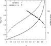 |
Fig. B.1 Decimal logarithm of the hypergeometric function 2F1 (u) (black line) appearing in Eq. (6), and total number of terms in the Taylor series required to reach the computer precision, i.e. 16 digits (right axis). This number can be reduced by a factor two for a 8-digit precision; see Sec. B. The parameter is γ ≈ 1.89 corresponding to iron (see Table 1). |
Appendix C Coefficients ci fitting the mass–radius relationship for single-layer planets (static case)
Appendix D Coefficients cij fitting the mass–radius relationship for single-layer planets
Appendix 5 Coefficients tij fitting the period for single-layer planets
Appendix F Mass-radius relationship for two-layer IP planets
Appendix G Mass-radius relationship for two-layer, PW planets
Appendix H Coefficients fitting the mass–radius relationship for two-layer IW planets
Coefficients c′i for the mass–radius relationship fitted with a quadratic law for a two-layer, IW planet for different values of q, in the static case⋆.
Coefficients d0, d1, and d2 for the sigmoidal representation of c′0(q) for the IW planet, assuming σ is a constant.
Appendix I Coefficients fitting the mass–radius relationship for two-layer IW, IP, and PW planets
 |
Fig. I.1 Mean coefficients |


Coefficients⋆ c′ij, dij and σ.
Appendix J Central pressure and rotation periods for the IP and PW planets
The notation differs slightly from Seager et al. (2007) where Eq. (4) is written as ρ = ρ0 + cPn. The connection between the two formula requires ρ0 → ρs, n → m and c → K-m. As a consequence, if the pressure P is measured in dyn/cm2, then the values of K-m reported in Table 1 are in g/cm3 × (dyn/cm2)-m.
DOI:10.5281/zenodo.15397897. Specific runs can be provided upon request. The presence of 2F1 (u) in Eq. (6) largely increases the computing time with respect to a standard polytropic EoS (see Appendix B for a discussion about convergence acceleration and the computing time). The production of each cube of data requires about 6 h of computation on a standard computer for a two-layer configuration.
All Tables
Example of data set* for a pure water planet with f = 0.1 (top) and for IW planet with f = 0.1 and q = 0.5 (bottom).
Coefficients c′i for the mass–radius relationship fitted with a quadratic law for a two-layer, IW planet for different values of q, in the static case⋆.
Coefficients d0, d1, and d2 for the sigmoidal representation of c′0(q) for the IW planet, assuming σ is a constant.
All Figures
|
Fig. 1 Typical configuration and notations for a rotating system made of L = 2 differentiated layers: the core (C) as layer 1, and the envelope (E) as layer 2. The polar radius is Rpol ≡ Z2 and the equatorial radius is Req ≡ R2. All layers rotate at the same rate Ω around the Z-axis. |
| In the text | |
|
Fig. 2 Normalised pressure (left) and mass-density (right) in colour code (top) close to the pole and to the equator for a two-layer, IP planet computed with the DROP code. The input and output parameters are in Table 2. Profiles along the rotation axis (spherical radius r ≡ Z) and along the equator (r ≡ R) are also shown (bottom). |
| In the text | |
|
Fig. 3 Mass–radius relationships (left axis) computed with the DROP code in the single layer case, for iron (purple), perovskite (green), and water (cyan), and for three flattening parameters, f ∈> {0,0.1,0.2}. Values of the input parameter A are indicated along the curves for f = 0, as described in Eq. (8). The domain where the fits are performed is indicated (grey-shaded zone) as well as the absolute error (right axis). The result obtained with ρs = 1 g/cm3, f = 0 and A = 0.6 for water in Eq. (4) is shown for comparison (cyan open circle). Also plotted are the empirical relationship valid in the range 1-8 M⊕ and built from the Earth’s model by Zeng et al. (2016) (black crosses), the data from Table B.1 of Haldemann et al. (2020) obtained from the AQUA-EoS for water assuming a 300 K surface temperature (thin, dotted lines) and the results by Fortney et al. (2007) for pure-water and pure-silicate planets (open and filled squares), all obtained in the static case. See Sect. 6 for a discussion about LHS 1140 b (red dot). |
| In the text | |
|
Fig. 4 Central pressure, Pc, in the same conditions as for Fig. 3 for f ∈ {0,0.1,0.2} and the classical estimate P0 for spherical systems (dashed line) according to Eq. (19). |
| In the text | |
|
Fig. 5 Rotation period, T, of single-layer planets in the same conditions as for Fig. 3 for f = 0.1, together with the fit with Eq. (21). The period of the Maclaurin spheroid (dotted lines) having with the same flattening and same mean mass density according to Eq. (20) is also given. |
| In the text | |
|
Fig. 6 Same caption as for Fig. 3, but in a two-layer IW planet, in the static case. Labels refer to values of top-to-bottom mass density ratio A (single-layer) and the relative size of the core q along the sequences. The effect of rotation is also shown for f = 0.2 (bottom right, red lines; a vertical shift of -0.6 applied for clarity). |
| In the text | |
|
Fig. 7 Coefficient c′0 obtained in the IW case fitting the mass-radius relationship for a given value of the core fractional size, q, for each flattening parameter, f (dots). The fits by a sigmoid are superimposed (plain lines), and the absolute error is also shown (dashes lines, right axis). |
| In the text | |
|
Fig. 8 Parameters ηr (top), ηm (bottom) and ηq (bottom) measuring the relative change in the equatorial radius, mass and core fraction respectively with rotation (in units of f) as a function of the core size q for 0.1 Me, 1 Me, and 10Me. |
| In the text | |
|
Fig. 9 Core mass-fraction versus the mass for the IW planet in the static case (colour gradient) and for f = 0.2 (red). See Appendix J for the IP and PW planets. |
| In the text | |
|
Fig. 10 Same caption as for Fig. 9, but for the period T computed for f = 0.1; see Appendix J for the IP and PW planets. |
| In the text | |
|
Fig. 11 Four sets of fiducial data (M ± δM, Req ± δReq) placed in the mass-radius relationship for IW planets (left panels) for M = 1M⊕, and Req = 1.3 R⊕ (top) and Req = 0.85 R⊕ (bottom). Error bars are δM/M = 0.1 and δReq/Req = 0.02 (black, plain lines) and δM/M = 0.02 and δReq/Req = 0.1 (black, dotted lines). The image of the error bars in terms of fractional size q is shown in the static case (middle panels) and with fast rotation f = 0.2 (right panels). See also Fig. 6. |
| In the text | |
|
Fig. 12 Position of LHS 1140 b (red) in the mass–radius diagrams for single-layer, pure-perovskite planets obtained for different flattening parameters. The A-sequence obtained with the DROP code for f = 0.055 is also plotted (black); see Fig. 3. |
| In the text | |
|
Fig. 13 Position of LHS 1140 b (red) in the mass–radius diagram for IW planets (top), for IP planets (middle) and for PW planets (bottom). The one-sigma error bars are taken from (Cadieux et al. 2024a). The best static A-sequence is also plotted for IW and PW configurations (black). See also Fig. 15 and Table 5. |
| In the text | |
|
Fig. 14 Structure parameters of LHS 1140 b compatible with the error bars (see Fig. 13, top panel) computed with the DROP code, assuming a two-layer, IW planet in three rotational states. The colour code refers to values of the core fractional size, which is smaller in the static case than with rotation; see also Fig. 6. Regarding the ocean depth, see Sect. 7.3. As an indication of the break-up velocity (which depends on q), we have reported in the last panel the Keplerian period at the planet equator (red) as well as the period associated with δf = 0.029, which amplitude corresponds to the error bars in the static case; see Eq. (36). |
| In the text | |
|
Fig. 15 Same caption as in Fig. 2 but for LHS 1140 b, assuming a rotating IP planet with q = 0.15 and f = 0.05. See also Table 5 and Fig. 13 (middle panel). |
| In the text | |
|
Fig. 16 Two extreme orientations of the rotation axis of the planet with respect to the line of sight (perpendicular to the figure) during a transit, relative to the spherical case. |
| In the text | |
|
Fig. 17 Effective position of LHS 1140 b in the PW diagram if the rotation axis of the planet is perpendicular to the line-of sight, corresponding to an oblate transit for f = 0.05. See also Figs. 13 (bottom) and 16. |
| In the text | |
|
Fig. 18 Same caption as for Fig. 15 but assuming a PW planet and an oblate transit with f = 0.05 (the period is T ≈ 6 h). See also Table 7 and Fig. 17. |
| In the text | |
|
Fig. B.1 Decimal logarithm of the hypergeometric function 2F1 (u) (black line) appearing in Eq. (6), and total number of terms in the Taylor series required to reach the computer precision, i.e. 16 digits (right axis). This number can be reduced by a factor two for a 8-digit precision; see Sec. B. The parameter is γ ≈ 1.89 corresponding to iron (see Table 1). |
| In the text | |
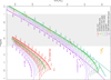 |
Fig. F.1 Same caption as for Fig. 6 but in a two-layer IP planet. |
| In the text | |
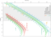 |
Fig. G.1 Same caption as for Fig. 6 but in a two-layer PW planet. |
| In the text | |
|
Fig. I.1 Mean coefficients |
| In the text | |
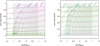 |
Fig. J.1 Same caption as for Fig. 9, but for the IP planet (left) and for the PW planet (right). |
| In the text | |
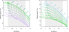 |
Fig. J.2 Same caption as for Fig. 10, but for the IP planet (left) and for the PW planet (right). |
| In the text | |
Current usage metrics show cumulative count of Article Views (full-text article views including HTML views, PDF and ePub downloads, according to the available data) and Abstracts Views on Vision4Press platform.
Data correspond to usage on the plateform after 2015. The current usage metrics is available 48-96 hours after online publication and is updated daily on week days.
Initial download of the metrics may take a while.