| Issue |
A&A
Volume 701, September 2025
|
|
|---|---|---|
| Article Number | A118 | |
| Number of page(s) | 17 | |
| Section | Planets, planetary systems, and small bodies | |
| DOI | https://doi.org/10.1051/0004-6361/202554339 | |
| Published online | 09 September 2025 | |
Collisional evolution of Jupiter trojans after capture: Insights into their origin and cratering record
1
Departamento de Física, Ingeniería de Sistemas y Teoría de la Señal, Escuela Politécnica Superior, Universidad de Alicante,
03690
Sant Vicent del Raspeig (Alicante),
Spain
2
Instituto de Física Aplicada a las Ciencias y la Tecnologías, Universidad de Alicante,
03690
Sant Vicent del Raspeig (Alicante),
Spain
3
Faculdade de Ciências e Tecnologias, Universidade de Coimbra,
Portugal
4
Institut de Ciències del Cosmos (ICCUB), Universitat de Barcelona (IEEC-UB),
Carrer de Martí i Franquès, 1,
08028
Barcelona,
Spain
★ Corresponding author: This email address is being protected from spambots. You need JavaScript enabled to view it.
Received:
1
March
2025
Accepted:
1
July
2025
Abstract
Context. Jupiter trojans (JTs) are asteroids that populate the Sun–Jupiter Lagrangian regions L4 and L5. This population is believed to be made up of leftovers from the Solar System’s early days that have remained in stable orbits around Jupiter for billions of years after their capture.
Aims. We investigated the long-term collisional evolution and the expected cratering record of the JT population under different initial conditions to assess whether these results are compatible with setting its origin in the primordial outer planetesimal disk.
Methods. We developed a dedicated numerical tool for this study by adapting the ALICANDEP code package, originally designed for trans-Neptunian objects, to the specific dynamical and physical environment of JTs. We also implemented updated scaling laws in the fragmentation algorithm to better capture the parameters dependency governing collisional physics. We validated the resulting model by comparing the output with previous results reported in the literature.
Results. Our findings support the hypothesis that JT formed in the primordial outer belt before being captured by Jupiter during the instability of the giant planets. The cratering record study demonstrates that material properties and cratering scaling law parameters can strongly influence the modelled crater distribution, with variations in strength and porosity affecting the saturation levels and crater sizes. This study provides insights into the collisional history of JTs and offers predictions for interpreting cratering data from the Lucy mission (NASA).
Key words: Kuiper belt: general / minor planets, asteroids: general / Kuiper belt objects: individual: Jupiter trojans
© The Authors 2025
 Open Access article, published by EDP Sciences, under the terms of the Creative Commons Attribution License (https://creativecommons.org/licenses/by/4.0), which permits unrestricted use, distribution, and reproduction in any medium, provided the original work is properly cited.
This article is published in open access under the Subscribe to Open model. This email address is being protected from spambots. You need JavaScript enabled to view it. to support open access publication.
1 Introduction
Jupiter trojans (JTs or trojans hereafter) are populations of small asteroids that share the orbit of Jupiter around the Sun. At a mean distance of about 5.2 au, JTs occupy two stable regions around the L4 and L5 Lagrange equilibrium points of the restricted three-body problem in the rotating system of Jupiter around the Sun. One of the most intriguing aspects of JT is the puzzle behind its origin. This population is believed to have formed in the early Solar System, with its current orbits being the result of a complex interplay in its gravitational interaction with Jupiter and other giant planets (Nesvorný et al. 2018; Morbidelli & Nesvorný 2020).
Various mechanisms have been proposed regarding the origin of the trojan population (see Emery et al. (2015) for a review). One of the prevailing theories explaining the origin of JTs involves the capture of planetesimals during the giant planets instability phase (Nesvorný et al. 2018; Bottke et al. 2023a). One particularly successful hypothesis is the ’jumping capture’ model proposed by Nesvorný et al. (2013). Such a model builds upon the ’chaotic capture’ model previously proposed by Morbidelli et al. (2005). According to Nesvorný et al. (2013), Jupiter orbit was scattered multiple times by encounters with an ice giant, causing the planet Lagrangian regions to shift in semi-major axis (Nesvorný & Morbidelli 2012). As a result, these regions eventually covered a populated area of planetesimals, capturing them in the process. This model not only reproduces the orbital distribution of JTs, but also offers a potential explanation for the asymmetric abundances of the leading and trailing populations confirmed by Uehata et al. (2022). An alternative model proposed by Pirani et al. (2019a,b) suggests that Jupiter formed at a distance of about 20 au or further and migrated to its current location while growing in mass, sweeping up planetesimals, and capturing JT in the 1:1 resonance. This model accounts for the asymmetry in the size of the two trojan swarms, but the captured bodies do not match the observed masses or inclinations of the observed trojans. The trojans will be visited by the Lucy space mission (NASA) to help unravel the origin of such an intriguing population (Levison et al. 2021).
Jupiter trojans have experienced significant collisional evolution since their capture, evidenced by the presence of nine collisional families in the L4 swarm and four in the L5 swarm, according to a recent update by Vokrouhlický et al. (2024). Although previous studies investigated the collisional dynamics of JTs, many were conducted before the publication of the capture model (i.e. Marzari et al. 1997; de Elía & Brunini 2007). Consequently, the initial conditions assumed previously, including the initial size distribution of the population and the physical parameters governing collisional responses, should be revisited. To address this, recent studies such as those of Marschall et al. (2022) and Bottke et al. (2023b) have examined the collisional evolution of JTs within the context of the giant planet instability scenario. Using the Boulder code (Morbidelli et al. 2009), both investigations modelled the evolved size-frequency distribution (SFD) of trojans. Marschall et al. (2022) revealed that an unconventional weak collisional strength, with a minimum at 20 m, could ensure the survival of satellites like Queta (3548 Eurybates), over the age of the Solar System. Lately, Bottke et al. (2023b) suggested that an even weaker scaling law is necessary to match the SFD of a trojan population originating from the primordial outer belt, located just behind Neptune when the planet started migrating.
When investigating the collisional evolution of JTs, it is important to consider that its initial population may have been eroded early, before it left the primordial outer belt (in the framework of JT captured by Jupiter during the giant planet instability phase). Benavidez et al. (2025; B25 hereinafter) employed ALICANDEP-22 to model the collisional evolution of the primordial belt and the subsequent evolution of the Kuiper Belt populations, including insights from recent findings by the Outer Solar System Survey (OSOSS) (Petit et al. 2023). The OSOSS analysis showed a striking similarity in the shape of the SFD for the dynamically hot and cold components of the Kuiper Belt within a specific magnitude range Hr ≈ 5.3 to 8.3 (Kavelaars et al. 2021; Petit et al. 2023). As proposed by these authors, this hints at a potential common formation mechanism in the corresponding diameter range of 100 < D < 400 km. Simultaneously, Lyra et al. (2023) highlighted the significance of poly-disperse pebble accretion following streaming instability in planetesimal formation, indicating that such a process led to the accretion of bodies up to several hundred kilometres in diameter at heliocentric distances reaching the current location of the cold Kuiper Belt (CKB). B25 blended such improvements and demonstrated that under suitable conditions, it is feasible to reproduce the present-day size-frequency distribution of both the hot and cold components of the Kuiper Belt.
Building upon the work of B25, we propose to continue their study in this paper. Here, we model the collisional evolution of JT using as input a fraction of the early evolved outer belt at the onset of the giant planets instability. Additionally, we investigate the history of cratering on bodies with sizes equivalent to the targets of the Lucy mission.
This paper is organised as follows. Section 2 introduces the methodology used to model the collisional evolution, giving an overview of our ALICANDEP-JT code. Section 3 compares ALICANDEP-JT results with previous models under the same or equivalent conditions. In Section 4, we present our new results for modelling the collisional evolution of JT under the capture hypothesis. Finally, Section 5 summarises our results and discusses their implications.
2 Methods
In this study, we used ALICANDEP-JT, a simplified version of the code ALICANDEP (Benavidez & Campo Bagatin 2009; Campo Bagatin & Benavidez 2012), adapted to track the evolution of a single zone. The collisional evolution code ALICANDEP-JT is divided into two components: the first component is an algorithm determining the impact outcome of cratering, fragmentation, and re-accumulation, following collisions between two bodies of any given size, within the size range under study. Then, the main code component models the collisional evolution of a given initial population over time.
2.1 Impact outcome
In this section, we outline the essential features of the first component of the model, based on the Petit & Farinella (1993) algorithm to model the cratering and fragmentation processes with the improvements introduced by O’Brien & Greenberg (2005). For further details, we recommend referring to Petit & Farinella (1993).
The main output of the algorithm is the fragmentation matrix f(i,j,k), which is used as input in the following evolution equations. Such a matrix is a three-dimensional (3D) array containing the number of fragments of any size resulting from all possible collisions between two bodies of diameters d(i) and d(j). For any single collision between two bodies of given masses (Mi, Mj), at some relative velocity (Vrel), their relative kinetic energy (Erel) can be compared with the threshold shattering energy of each colliding body to determine the outcome: cratering or shattering. The relative kinetic energy is:
![Mathematical equation: $\[E_{\mathrm{rel}}=\frac{M_i M_j ~V_{\mathrm{rel}}^2}{2\left(M_i+M_j\right)}.\]$](/articles/aa/full_html/2025/09/aa54339-25/aa54339-25-eq1.png) (1)
(1)
The impact kinetic energy is assumed to be equally partitioned between the two colliding bodies. Fragmentation occurs if:
![Mathematical equation: $\[E_{\mathrm{rel}}>2 Q_S^* ~M_i,\]$](/articles/aa/full_html/2025/09/aa54339-25/aa54339-25-eq2.png) (2)
(2)
where ![Mathematical equation: $\[Q_{S}^{*}\]$](/articles/aa/full_html/2025/09/aa54339-25/aa54339-25-eq3.png) is the threshold specific energy for shattering, defined as the kinetic impact energy per unit mass of the target such that the impact produces the largest fragment with half the mass of the original target. The occurrence of a cratering event is a direct result of reversing the condition in Eq. (2). Thus, an abrupt transition from cratering to shattering regime is assumed, in agreement with a wealth of literature on shattering experiments, as in Fujiwara et al. (1977).
is the threshold specific energy for shattering, defined as the kinetic impact energy per unit mass of the target such that the impact produces the largest fragment with half the mass of the original target. The occurrence of a cratering event is a direct result of reversing the condition in Eq. (2). Thus, an abrupt transition from cratering to shattering regime is assumed, in agreement with a wealth of literature on shattering experiments, as in Fujiwara et al. (1977).
Generally speaking, when two bodies collide, there are three possible outcomes: (i) both objects are shattered; (ii) one body is shattered, while the other is cratered; or (iii) both objects are cratered. The latter case is limited to low-velocity collisions, which are not expected to take place in the JT system. In each case, the size distribution of fragments from each body needs to be calculated and combined to determine the final size distribution after computing the eventual fragment re-accumulation by self-gravity.
In impacts with a specific energy larger than the critical specific energy threshold for shattering, the mass fraction of the largest fragment with respect to the target mass is given by
![Mathematical equation: $\[f_{l, i}=M_{\max, i} / M_i,\]$](/articles/aa/full_html/2025/09/aa54339-25/aa54339-25-eq4.png) (3)
(3)
where fl,i is a function of the specific impact energy (![Mathematical equation: $\[Q_{S}^{*}\]$](/articles/aa/full_html/2025/09/aa54339-25/aa54339-25-eq5.png) ), the target mass (Mi), and the relative kinetic energy (Erel). It can be determined as follows.
), the target mass (Mi), and the relative kinetic energy (Erel). It can be determined as follows.
Shattering events (Erel >2![Mathematical equation: $\[Q_{S}^{*}\]$](/articles/aa/full_html/2025/09/aa54339-25/aa54339-25-eq6.png) Mi):
Mi):
![Mathematical equation: $\[f_{l, i}=\frac{1}{2}\left(\frac{Q_{S, i} M_{i}}{E_{\mathrm{rel}} / 2}\right)^{1.24}\]$](/articles/aa/full_html/2025/09/aa54339-25/aa54339-25-eq7.png) ,
,The mass distribution of fragments follows a power law with an exponent, bi, which is related to fl,i and estimated by a numerical approach (see Eq. (9) in Petit & Farinella 1993);
Cratering events (Erel < 2![Mathematical equation: $\[Q_{S}^{*}\]$](/articles/aa/full_html/2025/09/aa54339-25/aa54339-25-eq8.png) Mi):
Mi):
The largest surviving body always has a mass of Mi − Mcrat, where Mcrat is the mass excavated from the crater and converted into ejected fragments. This is calculated based on the values of Erel and α, the excavation coefficient of the impact, which depends on the material properties. Following Petit & Farinella (1993), we assume α = 1 × 10⁻⁴ s2/m2. Thus Mcrat can be calculated as:
![Mathematical equation: $\[\begin{aligned}& M_{\text {crat }}=\alpha E_{\text {rel }} \text { for } \quad E_{\text {rel }} \leq \frac{M_1}{100 \alpha}, \\& M_{\text {crat }}=\frac{9 \alpha}{200 Q_S \alpha-1} E_{\text {rel }}+\frac{M_i}{10} \frac{1-20 Q_S \alpha}{1-200 Q_S \alpha} \text { for } \frac{M_i}{100 \alpha}>E_{\text {rel}};\end{aligned}\]$](/articles/aa/full_html/2025/09/aa54339-25/aa54339-25-eq9.png)
The mass distribution of fragments follows a single slope power law with an exponent bi with a constant value of 0.8 (Melosh 1989);
-
The mass fraction of the largest fragment originated from the crater is
![Mathematical equation: $\[f_{l, i}=1-b_i+b_i f_{l, i}^{b_i}\left(\frac{M_{d u s t}}{M_i}\right)^{1-b_i},\]$](/articles/aa/full_html/2025/09/aa54339-25/aa54339-25-eq10.png)
where Mdust is the lower cutoff of the fragment mass produced distribution.
2.1.1 Re-accumulation model
A collision is always assumed to produce a remnant body comprising the two largest fragments from the colliding bodies. Apart from the largest remnant of each body, a collision also results in a distribution of smaller fragments which acquire non-negligible velocities. Thus, after any collision, each small fragment may either be re-accumulated back on the largest remnant or escape its gravitational potential.
Thus, as explained in Petit & Farinella (1993), using the energy balance equation allows us to compute the escape velocity, as
![Mathematical equation: $\[\frac{1}{2}\left(M_1-M_{max, 1}+M_2-M_{max, 2}\right) v_{e s c}^2+W_{t o t}=W_{f r, 1}+W_{f r, 2}+W_h,\]$](/articles/aa/full_html/2025/09/aa54339-25/aa54339-25-eq11.png) (4)
(4)
where Wtot is the total potential energy of the two bodies just before fragmentation, given by:
![Mathematical equation: $\[W_{t o t}=-\frac{3 G M_1^{5 / 3}}{5 Q_1}-\frac{3 G M_2^{5 / 3}}{5 Q_2}-\frac{G M_1 M_2}{Q_1 M_1^{1 / 3}+Q_2 M_2^{1 / 3}},\]$](/articles/aa/full_html/2025/09/aa54339-25/aa54339-25-eq12.png) (5)
(5)
where Qi is given by
![Mathematical equation: $\[Q_i=\left(\frac{4 \pi \rho_i}{3}\right)^{-1 / 3}.\]$](/articles/aa/full_html/2025/09/aa54339-25/aa54339-25-eq13.png)
Wfr,i is the sum of the self-gravitation potential energy of each fragment of body, i, given by
![Mathematical equation: $\[\begin{aligned}W_{f r, i} & =\frac{3 G}{5 Q_i} \int_{m=0}^{m=\infty} m^{5 / 3} n_i(m) d m \\& =-\frac{3 G}{5 Q_i} \frac{5 M_{max, i}^{5 / 3}-3 b_i M_{max, i}^{b_i} M_{dust}^{5 / 3-b_i}}{5-3 b_i},\end{aligned}\]$](/articles/aa/full_html/2025/09/aa54339-25/aa54339-25-eq14.png)
and Wh is an estimate of the potential energy when the fragments are separated by a distance of the order of the Hill’s radius.
Here, we include the corrections made by O’Brien & Greenberg (2005) to compute Wh according to the impact outcome. Thus, if both bodies are shattered, we have
![Mathematical equation: $\[W_h=-\frac{3 G\left(M_1+M_2\right)^{5 / 3}}{5} \frac{\left(3 M_{sun}\right)^{1 / 3}}{R_0}.\]$](/articles/aa/full_html/2025/09/aa54339-25/aa54339-25-eq15.png) (6)
(6)
However, if one body is shattered and the other is cratered, we have
![Mathematical equation: $\[W_h=-\frac{3 G\left(M_1-M_{\text {crat}, 1}\right)^{2 / 3}\left(M_2+M_{\text {crat}, 1}\right)}{2} \frac{\left(3 M_{sun}\right)^{1 / 3}}{R_0}.\]$](/articles/aa/full_html/2025/09/aa54339-25/aa54339-25-eq16.png) (7)
(7)
In the case where both bodies are cratered, we have
![Mathematical equation: $\[\begin{aligned}W_h= & -3 G\left(M_1+M_2-M_{\text {crat}, 1}-M_{\text {crat}, 2}\right)^{2 / 3} \\& \frac{\times\left(M_{\text {crat}, 1}+M_{\text {crat}, 2}\right)}{2} \frac{\left(3 M_{sun}\right)^{1 / 3}}{R_0},\end{aligned}\]$](/articles/aa/full_html/2025/09/aa54339-25/aa54339-25-eq17.png) (8)
(8)
where Msun and R0 are the mass of the Sun and the orbital radius, which is on the order of 5.2 au for JTs.
Then, it is time to compute the number and mass of fragments in bins representing the distribution function. Mass bins are organised into Nbin logarithmic, discretised bins, having their central values scaled by a factor of 2, and their limits are scaled accordingly. The central mass values are given by the following geometric sequence:
![Mathematical equation: $\[m_{b i n, k}=g^{k-1} m_{b i n, 1},\]$](/articles/aa/full_html/2025/09/aa54339-25/aa54339-25-eq18.png) (9)
(9)
where g = 2 and k is the bin number. Each bin spans the range of
![Mathematical equation: $\[\frac{m_{b i n, k}}{\sqrt{g}}, m_{b i n, k} \sqrt{g}.\]$](/articles/aa/full_html/2025/09/aa54339-25/aa54339-25-eq19.png) (10)
(10)
Therefore, neighbouring mass bins scale by a factor of 2, and bodies in bin k + 3 are twice the size of those in bin k.
Petit & Farinella (1993) defined the total kinetic energy of ejecta from body i as Efr,i = fke Erel/2, where fke is the fraction of the impact energy that is partitioned into kinetic energy of the fragments (see Sect. 2.1.3 for a new approach to this parameter).
Our model assumes a cumulative distribution for the fraction of mass larger than a given value, V:
![Mathematical equation: $\[f(>V)=\left(\frac{V}{V_{min }}\right)^{-K},\]$](/articles/aa/full_html/2025/09/aa54339-25/aa54339-25-eq20.png) (11)
(11)
where the exponent takes the value K = 9/4 (Gault et al. 1963) and Vmin is a fixed lower cutoff to the ejection velocity. Choosing a V value equal to the escape velocity allows us to find the fraction of escaping mass from the target (Campo Bagatin et al. 2001).
The fraction of re-accumulated mass is determined in the following way. If the number of fragments in a given size bin is less than 100, the velocity of each fragment is drawn at random from a Maxwellian velocity distribution:
![Mathematical equation: $\[P\left(v; V_0\right)=\sqrt{\frac{2}{\pi}} \frac{\sqrt{3} v^2}{V_0^3} \exp \left(-\frac{3 v^2}{2 V_0^2}\right),\]$](/articles/aa/full_html/2025/09/aa54339-25/aa54339-25-eq21.png) (12)
(12)
where v is the impact speed and ![Mathematical equation: $\[V_{0}^{2}=\left\langle v^{2}\right\rangle\]$](/articles/aa/full_html/2025/09/aa54339-25/aa54339-25-eq22.png) is the rms velocity value. Otherwise, if the number of fragments in the bin is larger than 100, the fraction of non-escaping fragments is calculated as:
is the rms velocity value. Otherwise, if the number of fragments in the bin is larger than 100, the fraction of non-escaping fragments is calculated as:
![Mathematical equation: $\[f=\int_0^{V_{e s c}} P\left(v; V_0\right) d v,\]$](/articles/aa/full_html/2025/09/aa54339-25/aa54339-25-eq23.png) (13)
(13)
where Vesc is the escape velocity.
2.1.2 Scaling laws for shattering and disruption
Scaling laws are mathematical expressions derived from observations, experiments, and shattering modelling, intended to extend the validity of experimental and modelling outcomes beyond the original studied size range. A scaling law depends on multiple parameters involved in the collision process: impact speed, material properties, density, gravitational forces, and so on. It comprises a set of parameters that is a function of the target diameter.
Over the years, several scaling laws were proposed, either in terms of threshold impact strength (S0) for shattering (i.e. Davis et al. 1985; Housen & Holsapple 1990) or in terms of disruption specific energy (![Mathematical equation: $\[Q_{D}^{*}\]$](/articles/aa/full_html/2025/09/aa54339-25/aa54339-25-eq24.png) ). The former was mainly derived from experiments, the latter was derived from numerical simulations. Here,
). The former was mainly derived from experiments, the latter was derived from numerical simulations. Here, ![Mathematical equation: $\[Q_{D}^{*}\]$](/articles/aa/full_html/2025/09/aa54339-25/aa54339-25-eq25.png) represents the threshold specific energy required to disperse the target into a spectrum of individual fragments but possibly re-accumulated, the largest fragment having exactly half of the mass of the original target. Benz & Asphaug (1999), through smoothed-particle hydrodynamics (SPH), self-consistently modelled this
represents the threshold specific energy required to disperse the target into a spectrum of individual fragments but possibly re-accumulated, the largest fragment having exactly half of the mass of the original target. Benz & Asphaug (1999), through smoothed-particle hydrodynamics (SPH), self-consistently modelled this ![Mathematical equation: $\[Q_{D}^{*}\]$](/articles/aa/full_html/2025/09/aa54339-25/aa54339-25-eq26.png) for a wide range of diameters. The result takes the functional form of
for a wide range of diameters. The result takes the functional form of
![Mathematical equation: $\[Q_D^*=A\left(\frac{R_T}{1 \mathrm{~cm}}\right)^a+B \rho\left(\frac{R_T}{1 \mathrm{~cm}}\right)^b,\]$](/articles/aa/full_html/2025/09/aa54339-25/aa54339-25-eq27.png) (14)
(14)
where A, a, B, b are constants determined for different target compositions and impact speeds, while RT is the target radius. The first term in Eq. (14) corresponds to the strength regime, where fragments cannot re-accumulate (the fragments are too dispersed and moving too fast to be held together by gravity). On the other hand, the second term corresponds to the gravity regime. This regime comes into play when the mass of the shattered target is large enough so that most ejected fragments cannot escape the gravitational potential well. In the gravity regime, fragments can re-accumulate and form gravitational aggregates (rubble piles).
O’Brien & Greenberg (2005) and de Elía & Brunini (2007) carried out collisional evolution simulations using the specific energy required for shattering a target into a spectrum of fragments, the largest one having exactly half the mass of the original target, denoted as ![Mathematical equation: $\[Q_{S}^{*}\]$](/articles/aa/full_html/2025/09/aa54339-25/aa54339-25-eq28.png) . Alternatively, a number of studies (Davis et al. 1985; Petit & Farinella 1993; Campo Bagatin et al. 1994, 2001; Benavidez & Campo Bagatin 2009, among others), have used a comparable approach focusing on impact strength, namely,
. Alternatively, a number of studies (Davis et al. 1985; Petit & Farinella 1993; Campo Bagatin et al. 1994, 2001; Benavidez & Campo Bagatin 2009, among others), have used a comparable approach focusing on impact strength, namely, ![Mathematical equation: $\[Q_{S}^{*}\]$](/articles/aa/full_html/2025/09/aa54339-25/aa54339-25-eq29.png) = S0/ρ.
= S0/ρ.
The units of ![Mathematical equation: $\[Q_{S}^{*}\]$](/articles/aa/full_html/2025/09/aa54339-25/aa54339-25-eq30.png) and
and ![Mathematical equation: $\[Q_{D}^{*}\]$](/articles/aa/full_html/2025/09/aa54339-25/aa54339-25-eq31.png) are energy per unit mass, which allows us to make a rough comparison of the two scaling laws, with caveats. In the strength regime, both coincide, as gravity does not contribute. The meaning of the rightmost branch (e.g. Fig. 1) of the two functions is different: In the case of
are energy per unit mass, which allows us to make a rough comparison of the two scaling laws, with caveats. In the strength regime, both coincide, as gravity does not contribute. The meaning of the rightmost branch (e.g. Fig. 1) of the two functions is different: In the case of ![Mathematical equation: $\[Q_{S}^{*}\]$](/articles/aa/full_html/2025/09/aa54339-25/aa54339-25-eq32.png) , the increase with size corresponds to the effect of gravitational self-compression. In the case of
, the increase with size corresponds to the effect of gravitational self-compression. In the case of ![Mathematical equation: $\[Q_{D}^{*}\]$](/articles/aa/full_html/2025/09/aa54339-25/aa54339-25-eq33.png) , the energy required to disperse fragments against the gravitational potential adds to self-compression, producing a noticeable difference between
, the energy required to disperse fragments against the gravitational potential adds to self-compression, producing a noticeable difference between ![Mathematical equation: $\[Q_{S}^{*}\]$](/articles/aa/full_html/2025/09/aa54339-25/aa54339-25-eq34.png) and
and ![Mathematical equation: $\[Q_{D}^{*}\]$](/articles/aa/full_html/2025/09/aa54339-25/aa54339-25-eq35.png) .
.
In an attempt to understand the link between ![Mathematical equation: $\[Q_{S}^{*}\]$](/articles/aa/full_html/2025/09/aa54339-25/aa54339-25-eq36.png) and
and ![Mathematical equation: $\[Q_{D}^{*}\]$](/articles/aa/full_html/2025/09/aa54339-25/aa54339-25-eq37.png) , de Elía & Brunini (2007) parameterised Eq. (14) as
, de Elía & Brunini (2007) parameterised Eq. (14) as
![Mathematical equation: $\[Q_D^*=C_1 D^{-\lambda_1}\left(1+\left(C_2 D\right)^{\lambda_2}\right).\]$](/articles/aa/full_html/2025/09/aa54339-25/aa54339-25-eq38.png) (15)
(15)
To reproduce the Benz & Asphaug (1999) scaling law for icy bodies with impact speeds of 3 km/s, the constant parameters C1, C2, λ1, and λ2 were set to values 24, 2.3, 0.39, and 1.65, respectively (to provide ![Mathematical equation: $\[Q_{D}^{*}\]$](/articles/aa/full_html/2025/09/aa54339-25/aa54339-25-eq39.png) in SI units). The idea was to have the possibility to examine a family of
in SI units). The idea was to have the possibility to examine a family of ![Mathematical equation: $\[Q_{S}^{*}\]$](/articles/aa/full_html/2025/09/aa54339-25/aa54339-25-eq40.png) identical to
identical to ![Mathematical equation: $\[Q_{D}^{*}\]$](/articles/aa/full_html/2025/09/aa54339-25/aa54339-25-eq41.png) in the strength regime, but with a lower value in the gravity regime. By varying the values of C2 and λ2 in Eq. (15), it is possible to create a family of
in the strength regime, but with a lower value in the gravity regime. By varying the values of C2 and λ2 in Eq. (15), it is possible to create a family of ![Mathematical equation: $\[Q_{S}^{*}\]$](/articles/aa/full_html/2025/09/aa54339-25/aa54339-25-eq42.png) that could be related to
that could be related to ![Mathematical equation: $\[Q_{D}^{*}\]$](/articles/aa/full_html/2025/09/aa54339-25/aa54339-25-eq43.png) . Therefore,
. Therefore, ![Mathematical equation: $\[Q_{S}^{*}\]$](/articles/aa/full_html/2025/09/aa54339-25/aa54339-25-eq44.png) is expressed as:
is expressed as:
![Mathematical equation: $\[Q_S^*=C_1 D^{-\lambda_1}\left[1+\left(C_2^{\prime} D\right)^{\lambda_2^{\prime}}\right],\]$](/articles/aa/full_html/2025/09/aa54339-25/aa54339-25-eq45.png) (16)
(16)
where ![Mathematical equation: $\[C_{2}^{\prime}\]$](/articles/aa/full_html/2025/09/aa54339-25/aa54339-25-eq49.png) and
and ![Mathematical equation: $\[\lambda_{2}^{\prime}\]$](/articles/aa/full_html/2025/09/aa54339-25/aa54339-25-eq50.png) are slight variations of the parameters C2 and λ2. In this work, we updated the Petit & Farinella (1993) algorithm, including Eq. (16) for the scaling law and tested values for
are slight variations of the parameters C2 and λ2. In this work, we updated the Petit & Farinella (1993) algorithm, including Eq. (16) for the scaling law and tested values for ![Mathematical equation: $\[C_{2}^{\prime}\]$](/articles/aa/full_html/2025/09/aa54339-25/aa54339-25-eq51.png) and
and ![Mathematical equation: $\[\lambda_{2}^{\prime}\]$](/articles/aa/full_html/2025/09/aa54339-25/aa54339-25-eq52.png) . The goal of this approach is to crumble the
. The goal of this approach is to crumble the ![Mathematical equation: $\[Q_{D}^{*}\]$](/articles/aa/full_html/2025/09/aa54339-25/aa54339-25-eq53.png) into a combination of factors as
into a combination of factors as ![Mathematical equation: $\[Q_{S}^{*}\]$](/articles/aa/full_html/2025/09/aa54339-25/aa54339-25-eq54.png) , fke (fraction of kinetic energy transferred to fragments) and reaccumulation processes. We give more details on this approach in Sect. 3.3.
, fke (fraction of kinetic energy transferred to fragments) and reaccumulation processes. We give more details on this approach in Sect. 3.3.
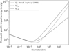 |
Fig. 1 Comparison of two selected scaling laws from EB07, |
![Mathematical equation: $\[Q_{S, a}^{*}\]$](/articles/aa/full_html/2025/09/aa54339-25/aa54339-25-eq46.png)
![Mathematical equation: $\[Q_{S, b}^{*}\]$](/articles/aa/full_html/2025/09/aa54339-25/aa54339-25-eq47.png)
![Mathematical equation: $\[Q_{D}^{*}\]$](/articles/aa/full_html/2025/09/aa54339-25/aa54339-25-eq48.png)
2.1.3 Fraction of kinetic energy transferred to fragments
An important parameter in the re-accumulation process is fke, defined as the fraction of impact energy that is transferred as kinetic energy of the produced fragments. This is directly related to its re-accumulation chances, after comparison with the gravitational potential energy of the rest of the mass.
Nonetheless, our knowledge of this parameter is very limited, as the available data are restricted to laboratory experiments on centimeter to decimeter targets sizes (Nakamura & Fujiwara 1991; Giblin et al. 2004), and to hydrocode experiments on targets with a diameter over a few hundreds of metres, such as that of Melosh & Ryan (1997). O’Brien & Greenberg (2005) suggested a power-law function for fke, depending on size (diameter):
![Mathematical equation: $\[f_{k e}=f_{k e_0}\left(\frac{D}{1000 \mathrm{~km}}\right)^\gamma,\]$](/articles/aa/full_html/2025/09/aa54339-25/aa54339-25-eq55.png) (17)
(17)
where γ is always between 0 and 1 and fke0 is the value at 1000 km. Suitable values of fke0 are in the range of 0.05 to 0.3 (Davis et al. 1989). de Elía & Brunini (2007) attempted to model the collisional evolution of the L4 swarm, using γ = 0.7 and fke0 = 0.35. These values generate an fke at smaller sizes that is not aligned with the experimental data (Nakamura & Fujiwara 1991; Giblin et al. 2004) (see Fig. 5). Therefore, in this work, we experimented with variations of Eq. (17), while comparing our model with other collisional models (see Sect. 3.3). Such a formulation allows for a more flexible use of both parameters, ![Mathematical equation: $\[Q_{S}^{*}\]$](/articles/aa/full_html/2025/09/aa54339-25/aa54339-25-eq56.png) and fke.
and fke.
2.2 Collisional evolution
The collisional evolution of a population of interacting bodies, including their mutual fragmentation, is performed by a set of n non-linear, second-order differential equations. Such equations can be numerically solved. The change per time step in the number of objects belonging to a given bin k is calculated as:
![Mathematical equation: $\[\Delta N(k)=\sum_i^n \sum_j^i P_{i n t} \cdot f(i, j, k) \cdot s(i, j) \cdot f_g \cdot \frac{\left(N(i)-\delta_{i j}\right) N(j)}{1+\delta_{i j}} \Delta t,\]$](/articles/aa/full_html/2025/09/aa54339-25/aa54339-25-eq57.png) (18)
(18)
where Pint is the intrinsic probability of collision inside the JT swarm, s(i, j) = 1/4 · (Di + Dj)2 is the impact cross-section and fg ≈ 1 + (Vesc/Vrel)2 accounts for the gravitational focusing increasing the cross-section. Therefore, the number of objects in bin k at time step t + δt is
![Mathematical equation: $\[N_k(t+\delta t)=N_k(t)+\delta t \cdot d N_k(t).\]$](/articles/aa/full_html/2025/09/aa54339-25/aa54339-25-eq58.png) (19)
(19)
The bin population is integrated in time through the Euler method, satisfying the following relation at each time step,
![Mathematical equation: $\[d N_k(t+\delta t)<\epsilon \cdot N_k(t),\]$](/articles/aa/full_html/2025/09/aa54339-25/aa54339-25-eq59.png) (20)
(20)
where 0 < ϵ < 1 is the parameter that specifies the fraction of the population in any bin k that should not be increased/decreased at each time step. Then, the code readjusts the time step (increasing or decreasing it) for the next iteration according to the actual difference in the number of objects. This feature avoids divergence in the evolution algorithm.
Campo Bagatin et al. (1994) noted a fictitious wavy pattern that can potentially extend across all size ranges in collisional evolution system. In their study, the authors elucidated that this structure arises due to a sharp cutoff or discontinuity at some small size. To neutralise the effect of such a wavy pattern, an artificial tail at small sizes was introduced in the distribution. The tail extends from the smaller limit assumed for fragments (Mdust) up to the first size bin selected as the lower limit for evolution. The role of the tail is only to provide projectiles to the smallest size range of bodies. Thus, the evolution of the tail itself is not performed. Instead, it is extrapolated through a power law, with a slope calculated from a set of the smallest size bins (e.g. 15, 20) in the evolving populations. This methodology is efficient and removes any artificial wavy structure.
In addition, the model includes the possibility to have either a constant relative impact velocity or a Maxwellian velocity distribution function. This feature can be toggled on or off according to specific requirements.
We considered only mutual collisions among L4 trojans, as previous studies have shown that the contribution of other projectile populations, such as Hilda asteroids and Jupiter-family comets (JFCs), is negligible. The intrinsic collision probabilities between these populations and the L4 trojans are more than an order of magnitude lower than those for trojan-trojan collisions – for instance, a factor of 24 and 26 lower for JFCs and Hildas, respectively (Dell’Oro & Paolicchi 1998; Dell’Oro et al. 2001). In addition, the number of potential impactors is significantly smaller: recent estimates suggest that the number of Hildas larger than 3 km (Zain et al. 2025; Vokrouhlický et al. 2025) is at least one order of magnitude smaller than the corresponding L4 trojan population (Wong & Brown 2015). As a result, their contribution to the collisional evolution is negligible compared to trojan-trojan collisions. While cometary impacts may have played a more significant role during a brief early phase after implantation (~10 Myr, Marchi et al. 2023), our model aims to characterise the long-term collisional evolution, during which any potential evidence of that transient phase may have been smoothed out.
Although our model does not explicitly track the dynamical evolution of fragments after collisions, we note that some ejected fragments may escape the L4 region if their post-impact orbits fall outside the stability zone. This loss mechanism has been investigated in previous studies. Marzari et al. (1995) initially suggested that up to ~20% of collisional fragments might leave the trojan clouds but later refined this estimate to ~10% based on improved modelling (Marzari et al. 1997). More recently, de Elía & Brunini (2007) applied a detailed orbital analysis and concluded that the escape rate is significantly lower, with about 50 bodies larger than 1 km leaving the L4 region per Myr. These results suggest that, although this mechanism exists, it likely represents a minor contribution to the overall mass loss and does not significantly impact the long-term collisional evolution. A broader discussion of this process can be found in the review by Emery et al. (2015).
3 Testing ALICANDEP-JT model
In this section, we describe how we used ALICANDEP-JT to reproduce the modelling results of two previous studies on the collisional evolution of JTs, namely, de Elía & Brunini (2007) (EB07, hereafter) and Marschall et al. (2022) (M22, hereafter). By comparing our results with EB07, we aim to validate our numerical model, while the comparison with M22 allows us to assess different approaches to the implemented scaling laws.
3.1 Comparison with previous JT collisional evolution models
First, we compared ALICANDEP-JT with de Elía & Brunini (2007). Since EB07 adopts a similar approach to the fragmentation and re-accumulation process to ALICANDEP-JT (as described in Sect. 2.1), this comparison serves to validate our code. Once this test was done, the next step was to understand how the combination of the ![Mathematical equation: $\[Q_{S}^{*}\]$](/articles/aa/full_html/2025/09/aa54339-25/aa54339-25-eq60.png) scaling law and the subsequent re-accumulation (influenced by fke) can produce results comparable to those of a model using
scaling law and the subsequent re-accumulation (influenced by fke) can produce results comparable to those of a model using ![Mathematical equation: $\[Q_{D}^{*}\]$](/articles/aa/full_html/2025/09/aa54339-25/aa54339-25-eq61.png) , such as M22. In all simulation runs discussed in Sect. 3, we used the same boundary conditions and parameters outlined in the referenced studies to perform analogous numerical simulations with our model, granting a consistent comparison.
, such as M22. In all simulation runs discussed in Sect. 3, we used the same boundary conditions and parameters outlined in the referenced studies to perform analogous numerical simulations with our model, granting a consistent comparison.
We carried out Kolmogorov–Smirnov (KS) tests to compare our results with previous studies. Such test compares two populations and determines whether two samples come from the same underlying population or have significantly different distributions. The test takes the two samples as input and returns two outcome values: namely, the test statistics (D) and the p-value. The D value is the maximum difference between the cumulative distribution functions of the two samples. It represents a measure of the discrepancy between the two distributions. The p-value represents the probability of observing the obtained D, or an even more extreme value, given that the null hypothesis is true. The null hypothesis is the assumption that the two samples are drawn from the same underlying population or have the same distribution. A minimum p-value significance level of 0.05 is commonly considered sufficient to retain the null hypothesis. However, a visual analysis is also useful because some patterns and details are invisible to a statistical test.
KS test statistics between EB07 and ALICANDEP-JT.
3.2 Comparison with de Elía & Brunini (2007)
Here, the initial population is defined by a cumulative SFD described by a broken power law with a transition diameter at 60 km. Thus, the starting cumulative SFD has a shallow slope, q = 3, for small bodies, and a steeper slope, q = 4.7, for larger bodies. The result is an initial population with a mass of 8.37 × 10⁻⁵ M⊕ (assuming a bulk density of 1500 kg m−3 for bodies), which is significantly more massive than the value predicted nowadays for the JT (~10−5M⊕) (Morbidelli et al. 2005; Vinogradova & Chernetenko 2015; Pitjeva & Pitjev 2020). To model the collisional evolution of the L4 swarm, EB07 considered a constant value for relative impact speed, 4.66 km s−1 and an intrinsic impact probability value: 7.79 × 10⁻¹⁸ km−2 yr−1 (Dell’Oro & Paolicchi 1998).
EB07 developed an algorithm based on Petit & Farinella (1993) to model the impact outcome, and used as reference the Benz & Asphaug (1999) scaling law corresponding to icy targets at 3 km/s impact velocity. To compare our results to those of EB07, we perform runs using several of their sixteen different scaling laws. Figure 2 illustrates two specific cases where the selected scaling laws, ![Mathematical equation: $\[Q_{S, a}^{*}\]$](/articles/aa/full_html/2025/09/aa54339-25/aa54339-25-eq64.png) and
and ![Mathematical equation: $\[Q_{S, b}^{*}\]$](/articles/aa/full_html/2025/09/aa54339-25/aa54339-25-eq65.png) , were derived from Eq. (16) with parameter values (
, were derived from Eq. (16) with parameter values (![Mathematical equation: $\[C_{2}^{\prime}\]$](/articles/aa/full_html/2025/09/aa54339-25/aa54339-25-eq66.png) ,
, ![Mathematical equation: $\[\lambda_{2}^{\prime}\]$](/articles/aa/full_html/2025/09/aa54339-25/aa54339-25-eq67.png) ) set to (1.2, 1.75) and (2.3, 1.25), respectively. These
) set to (1.2, 1.75) and (2.3, 1.25), respectively. These ![Mathematical equation: $\[Q_{S}^{*}\]$](/articles/aa/full_html/2025/09/aa54339-25/aa54339-25-eq68.png) scaling laws are plotted alongside the standard Benz & Asphaug (1999) scaling law for
scaling laws are plotted alongside the standard Benz & Asphaug (1999) scaling law for ![Mathematical equation: $\[Q_{D}^{*}\]$](/articles/aa/full_html/2025/09/aa54339-25/aa54339-25-eq69.png) (icy composition). It is important to note that
(icy composition). It is important to note that ![Mathematical equation: $\[Q_{D}^{*}\]$](/articles/aa/full_html/2025/09/aa54339-25/aa54339-25-eq70.png) and the
and the ![Mathematical equation: $\[Q_{S}^{*}\]$](/articles/aa/full_html/2025/09/aa54339-25/aa54339-25-eq71.png) family are not directly comparable as they describe different definitions (threshold specific energy for disruption vs. threshold specific energy for shattering).
family are not directly comparable as they describe different definitions (threshold specific energy for disruption vs. threshold specific energy for shattering).
Table 1 presents the D-statistic and the p-value for each case. Since the p-values for both cases are above a significance level of 0.05, we accept the null hypothesis, indicating that the distributions obtained using EB07 and ALICANDEP-JT are statistically indistinguishable. Furthermore, Fig. 2 shows a visual comparison of the cumulative SFD of two tested cases. The SFDs of both numerical models show similar features, with dips and peaks occurring at the same size ranges.
The selected sampled cases from EB07 provide highly consistent results. Both scaling laws ![Mathematical equation: $\[Q_{S, a}^{*}\]$](/articles/aa/full_html/2025/09/aa54339-25/aa54339-25-eq72.png) and
and ![Mathematical equation: $\[Q_{S, b}^{*}\]$](/articles/aa/full_html/2025/09/aa54339-25/aa54339-25-eq73.png) demonstrate excellent agreement with EB07, reinforcing the validation of our model.
demonstrate excellent agreement with EB07, reinforcing the validation of our model.
3.3 Comparison with Marschall et al. (2022)
The initial distribution used by M22 is characterised by a cumulative SFD given by a power law with a slope of q = 2.1 for small bodies, and a steeper slope (q ~ 4.5) for bodies larger than 100 km. That produces a less massive initial population compared to EB07 (4 × 10⁻⁶ M⊕, assuming a bulk density of 1000 kg/m3). Note that, at this stage, we are assuming identical initial conditions only for comparison purposes. Thus, the intrinsic impact probability is set to 7 × 10⁻¹⁸ km−2 yr−1 and the impact velocity is set to a unique value of 4.6 km s−1 (Davis et al. 2002; Nesvorný et al. 2018).
In Marschall et al. (2022) the impact outcome is based on SPH modelling combined with Parallel K-D tree GRAVity code (pkdgrav) following the methodology described in Bottke et al. (2005). The authors examined two distinct characteristic scaling laws based on Eq. (14). The first was inspired by the scaling law for basalt material proposed by Benz & Asphaug (1999) with a minimum at ~250 m, which they also scale by different factors. The second, referred to as the ‘unconventional’ scaling law, has a minimum at 20 m. This unconventional choice for the minimum of QD was originally proposed to better match the crater distribution observed on irregular and regular satellites of giant planets (see Bottke et al. 2023b; Bottke et al. 2024).
In this section, we consider two scaling laws for comparison with Marschall et al. (2022). In case 1, the applied scaling law is indicated by Q0, which is approximately 100 times weaker than the scaling law for basalt proposed by Benz & Asphaug (1999), with a minimum at 250 m. In case 2, the applied scaling law corresponds to the ‘unconventional’ one in M22, with a minimum at 20 m.
M22 employed a ![Mathematical equation: $\[Q_{D}^{*}\]$](/articles/aa/full_html/2025/09/aa54339-25/aa54339-25-eq82.png) scaling law (Eq. (14)), whereas our code utilises a
scaling law (Eq. (14)), whereas our code utilises a ![Mathematical equation: $\[Q_{S}^{*}\]$](/articles/aa/full_html/2025/09/aa54339-25/aa54339-25-eq83.png) scaling law (Eq. (16)); however, as it was stated in Sect. 2.1.2,
scaling law (Eq. (16)); however, as it was stated in Sect. 2.1.2, ![Mathematical equation: $\[Q_{D}^{*}\]$](/articles/aa/full_html/2025/09/aa54339-25/aa54339-25-eq84.png) sets an upper limit for
sets an upper limit for ![Mathematical equation: $\[Q_{S}^{*}\]$](/articles/aa/full_html/2025/09/aa54339-25/aa54339-25-eq85.png) . Here we test different values of
. Here we test different values of ![Mathematical equation: $\[C_{2}^{\prime}\]$](/articles/aa/full_html/2025/09/aa54339-25/aa54339-25-eq86.png) and
and ![Mathematical equation: $\[\lambda_{2}^{\prime}\]$](/articles/aa/full_html/2025/09/aa54339-25/aa54339-25-eq87.png) in Eq. (16), combined with the approach for fke described in Sect. 2.1.3, until we find a good match for the final SFD. A verification that
in Eq. (16), combined with the approach for fke described in Sect. 2.1.3, until we find a good match for the final SFD. A verification that ![Mathematical equation: $\[Q_{S}^{*}\]$](/articles/aa/full_html/2025/09/aa54339-25/aa54339-25-eq88.png) is consistent with
is consistent with ![Mathematical equation: $\[Q_{D}^{*}\]$](/articles/aa/full_html/2025/09/aa54339-25/aa54339-25-eq89.png) is always necessary (i.e.
is always necessary (i.e. ![Mathematical equation: $\[Q_{S}^{*}\]$](/articles/aa/full_html/2025/09/aa54339-25/aa54339-25-eq90.png) must always be smaller than
must always be smaller than ![Mathematical equation: $\[Q_{D}^{*}\]$](/articles/aa/full_html/2025/09/aa54339-25/aa54339-25-eq91.png) in the gravity regime). Figures 3 and 4 show the set of tested scaling laws. To check the influence of different parameters, one of the parameters is kept constant while the other is given different values. Figure 3a the shows scaling law, Q0, where
in the gravity regime). Figures 3 and 4 show the set of tested scaling laws. To check the influence of different parameters, one of the parameters is kept constant while the other is given different values. Figure 3a the shows scaling law, Q0, where ![Mathematical equation: $\[C_{2}^{\prime}\]$](/articles/aa/full_html/2025/09/aa54339-25/aa54339-25-eq92.png) is constant and
is constant and ![Mathematical equation: $\[\lambda_{2}^{\prime}\]$](/articles/aa/full_html/2025/09/aa54339-25/aa54339-25-eq93.png) is given three different values, while Fig. 3b shows the outcome corresponding to a constant
is given three different values, while Fig. 3b shows the outcome corresponding to a constant ![Mathematical equation: $\[\lambda_{2}^{\prime}\]$](/articles/aa/full_html/2025/09/aa54339-25/aa54339-25-eq94.png) and
and ![Mathematical equation: $\[C_{2}^{\prime}\]$](/articles/aa/full_html/2025/09/aa54339-25/aa54339-25-eq95.png) taking three different values. Figure 4 is the same as Fig. 3, but for the ‘unconventional’ scaling law. The influence of the explored scaling laws is explained in more detail later in this section.
taking three different values. Figure 4 is the same as Fig. 3, but for the ‘unconventional’ scaling law. The influence of the explored scaling laws is explained in more detail later in this section.
In Sect. 2.1.3, we mention that fke can be given as a function of diameter (Eq. (17)). Here, we further explore this concept by adding a constant term to the expression:
![Mathematical equation: $\[f_{k e}=f_{k e_0}\left(\frac{D}{1000 \mathrm{~km}}\right)^\gamma+\beta,\]$](/articles/aa/full_html/2025/09/aa54339-25/aa54339-25-eq96.png) (21)
(21)
where β is a positive constant added to match the results of the impact experiment (Nakamura & Fujiwara 1991; Giblin et al. 2004). Such an expression allows for a small but not negligible value of fke at small sizes, as opposed to the former formulation of that parameter, which vanished quickly within the same size range. In addition, γ can be adjusted to set the diameter at which the function separates the constant regime and the exponential regime.
Four combinations of parameters are explored to assess the influence of fke. Such combinations are listed in Table 2 and are represented in Figure 5. The first case corresponds to the parameters used by de Elía & Brunini (2007) (Eq. (17)). The second case uses the same equation with values of fke0 and γ in accordance with Melosh & Ryan (1997). Through hydrocode calculations, Melosh & Ryan (1997) studied the impact energy in the context of fragment dispersion of large bodies. They also present constraints on fke, namely a value of 0.1 at 1000 km and a D1/2 decrease for small bodies (O’Brien & Greenberg 2005). In the third case, the β term is implemented to fit the experimental data at small sizes (Eq. (21)) (Nakamura & Fujiwara 1991; Giblin et al. 2004), but still using the results from Melosh & Ryan (1997), i.e., the fke value at 1000 km and the γ value are the same. (At 1000 km: fke = fke0 +β = 0.1). Nakamura & Fujiwara (1991) carried out an experimental study on the velocity distribution of fragments after a collision with basalt and alumina spherical targets of 6 cm in diameter, and they found fke ~ 0.01. Giblin et al. (2004), in a similar study on icy, 15 cm diameter targets, found a wider range of fke values, still in the same order of magnitude as in Nakamura & Fujiwara (1991). Giblin et al. (2004) manufactured three different types of icy targets: two types of ‘rubble piles’ and one more compact snowball; combinations of these three types of target (each type including targets with slightly different masses in each collision event) combined with three types of projectile generate various initial conditions and, as a result, different fke. In the fourth case, an increase in the value of γ is explored to better fit the data from Marschall et al. (2022). Appendix A shows the results for all different combinations of parameters in Table 2, highlighting the need for the non-negligible β parameter used in this section.
When comparing our results with those of Marschall et al. (2022), it is important to acknowledge that multiple sets of runs for the same case may show changes due to random seeds employed in the Boulder code. Consequently, the single SFD provided by R. Marschall and used for comparison in our study represents a potential outcome of the same initial system state. Thus, Figures 10 and 13 in M22 show slight differences (up to a factor of 2) in the number of bodies at sizes smaller than a few kilometres. This dispersion is represented as a shaded region in Figures 6 and 7, emphasising the essential agreement of our results.
We conducted a Kolmogorov-Smirnov test to provide a robust comparison of the results obtained by both models. We notice that, for comparison, we used an SFD falling roughly in the middle of the evolved distributions by M22. The best agreement with the reference simulations is achieved with the parameter values ![Mathematical equation: $\[C_{2}^{\prime}\]$](/articles/aa/full_html/2025/09/aa54339-25/aa54339-25-eq103.png) = 0.3 and
= 0.3 and ![Mathematical equation: $\[\lambda_{2}^{\prime}\]$](/articles/aa/full_html/2025/09/aa54339-25/aa54339-25-eq104.png) = 1.6 for case 1 (Q0), and
= 1.6 for case 1 (Q0), and ![Mathematical equation: $\[C_{2}^{\prime}\]$](/articles/aa/full_html/2025/09/aa54339-25/aa54339-25-eq105.png) = 8 and λ′2 = 1.8 for case 2 (the unconventional scaling law). In both cases, with a suitable choice of the parameters defining fke and
= 8 and λ′2 = 1.8 for case 2 (the unconventional scaling law). In both cases, with a suitable choice of the parameters defining fke and ![Mathematical equation: $\[Q_{S}^{*}\]$](/articles/aa/full_html/2025/09/aa54339-25/aa54339-25-eq106.png) , the evolved SFDs closely match those in M22. Specifically, the corresponding
, the evolved SFDs closely match those in M22. Specifically, the corresponding ![Mathematical equation: $\[Q_{S}^{*}\]$](/articles/aa/full_html/2025/09/aa54339-25/aa54339-25-eq107.png) exhibits a minimum shifted toward larger sizes by a factor of 2 and a strength reduced by a factor of 2 relative to the reference
exhibits a minimum shifted toward larger sizes by a factor of 2 and a strength reduced by a factor of 2 relative to the reference ![Mathematical equation: $\[Q_{D}^{*}\]$](/articles/aa/full_html/2025/09/aa54339-25/aa54339-25-eq108.png) scaling law (see Figures 3b and 4b). The following two sections give a detailed comparison with M22 for case 1 and case 2, guiding in the identification of the combination of scaling law parameters that best reproduces the reference runs from M22 summarised above.
scaling law (see Figures 3b and 4b). The following two sections give a detailed comparison with M22 for case 1 and case 2, guiding in the identification of the combination of scaling law parameters that best reproduces the reference runs from M22 summarised above.
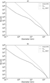 |
Fig. 2 Cumulative SFDs for cases |
![Mathematical equation: $\[Q_{S, a}^{*}\]$](/articles/aa/full_html/2025/09/aa54339-25/aa54339-25-eq74.png)
![Mathematical equation: $\[Q_{S, b}^{*}\]$](/articles/aa/full_html/2025/09/aa54339-25/aa54339-25-eq75.png)
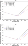 |
Fig. 3
|
![Mathematical equation: $\[Q_{S}^{*}\]$](/articles/aa/full_html/2025/09/aa54339-25/aa54339-25-eq76.png)
![Mathematical equation: $\[C_{2}^{\prime}\]$](/articles/aa/full_html/2025/09/aa54339-25/aa54339-25-eq77.png)
![Mathematical equation: $\[\lambda_{2}^{\prime}\]$](/articles/aa/full_html/2025/09/aa54339-25/aa54339-25-eq78.png)
![Mathematical equation: $\[\lambda_{2}^{\prime}\]$](/articles/aa/full_html/2025/09/aa54339-25/aa54339-25-eq79.png)
![Mathematical equation: $\[C_{2}^{\prime}\]$](/articles/aa/full_html/2025/09/aa54339-25/aa54339-25-eq80.png)
![Mathematical equation: $\[Q_{D}^{*}\]$](/articles/aa/full_html/2025/09/aa54339-25/aa54339-25-eq81.png)
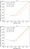 |
Fig. 4
|
![Mathematical equation: $\[Q_{S}^{*}\]$](/articles/aa/full_html/2025/09/aa54339-25/aa54339-25-eq97.png)
![Mathematical equation: $\[C_{2}^{\prime}\]$](/articles/aa/full_html/2025/09/aa54339-25/aa54339-25-eq98.png)
![Mathematical equation: $\[\lambda_{2}^{\prime}\]$](/articles/aa/full_html/2025/09/aa54339-25/aa54339-25-eq99.png)
![Mathematical equation: $\[\lambda_{2}^{\prime}\]$](/articles/aa/full_html/2025/09/aa54339-25/aa54339-25-eq100.png)
![Mathematical equation: $\[C_{2}^{\prime}\]$](/articles/aa/full_html/2025/09/aa54339-25/aa54339-25-eq101.png)
![Mathematical equation: $\[Q_{D}^{*}\]$](/articles/aa/full_html/2025/09/aa54339-25/aa54339-25-eq102.png)
Parameter values of fke function.
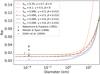 |
Fig. 5 Functions of fke tested and listed in Table 2. Black symbols correspond to values from Nakamura & Fujiwara (1991); Melosh & Ryan (1997); and Giblin et al. (2004), as indicated in the legend. |
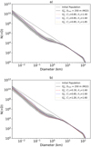 |
Fig. 6 Cumulative SFDs for runs corresponding to case 1, using the scaling laws showed in Figs. 3a and 3b). The fke function is determined by fke0 = 0.085, γ = 0.5 and β = 0.015. The solid black line is the evolved cumulative SFD using the scaling law, Q0, from Marschall et al. (2022) for visual comparison. |
3.3.1 Case 1: Q0 scaling law (Dmin = 250 m)
The scaling law, Q0, can be expressed by replacing parameters A, a, B and b in Eq. (14) by 1.50 × 106 erg g−1, −0.40, 1.30 erg cm3 g−2, and 1.30, respectively (Marschall et al. 2022). The same scaling law can be expressed as Eq. (15) using 1.9, 0.4, 2 and 1.7 in place of C1, λ1, C2 and λ2, respectively. For this scaling law, parameter ![Mathematical equation: $\[C_{2}^{\prime}\]$](/articles/aa/full_html/2025/09/aa54339-25/aa54339-25-eq109.png) is tested for values ranging from 0.3 to 1.2, combined with
is tested for values ranging from 0.3 to 1.2, combined with ![Mathematical equation: $\[\lambda_{2}^{\prime}\]$](/articles/aa/full_html/2025/09/aa54339-25/aa54339-25-eq110.png) , ranging from 1.4 to 1.85, in Eq. (16). The constant values for the fke function are fke0 = 0.085, γ = 0.5 and β = 0.015, which correspond to the best combination for this scaling law that match the reference run by M22 (Appendix A shows the results for all different parameter combinations in Table 2).
, ranging from 1.4 to 1.85, in Eq. (16). The constant values for the fke function are fke0 = 0.085, γ = 0.5 and β = 0.015, which correspond to the best combination for this scaling law that match the reference run by M22 (Appendix A shows the results for all different parameter combinations in Table 2).
Table 3 shows the combinations of ![Mathematical equation: $\[C_{2}^{\prime}\]$](/articles/aa/full_html/2025/09/aa54339-25/aa54339-25-eq111.png) and
and ![Mathematical equation: $\[\lambda_{2}^{\prime}\]$](/articles/aa/full_html/2025/09/aa54339-25/aa54339-25-eq112.png) explored in this study, along with the D and p-values for all runs. The statistical test outcomes indicate a substantial agreement between the evolved populations using ALICANDEP-JT and M22. The values of D are low, and the p-values consistently exceed the significance level, often approaching 1. As a result, comparing p-values may not help in determining the best run. Then, a visual inspection of the SFD is convenient at this stage.
explored in this study, along with the D and p-values for all runs. The statistical test outcomes indicate a substantial agreement between the evolved populations using ALICANDEP-JT and M22. The values of D are low, and the p-values consistently exceed the significance level, often approaching 1. As a result, comparing p-values may not help in determining the best run. Then, a visual inspection of the SFD is convenient at this stage.
Figure 6 shows the cumulative SFDs evolved under the ![Mathematical equation: $\[Q_{S}^{*}\]$](/articles/aa/full_html/2025/09/aa54339-25/aa54339-25-eq113.png) scaling laws presented in Fig. 3. All modelled SFD obtained for different combinations of
scaling laws presented in Fig. 3. All modelled SFD obtained for different combinations of ![Mathematical equation: $\[C_{2}^{\prime}\]$](/articles/aa/full_html/2025/09/aa54339-25/aa54339-25-eq114.png) and
and ![Mathematical equation: $\[\lambda_{2}^{\prime}\]$](/articles/aa/full_html/2025/09/aa54339-25/aa54339-25-eq115.png) can reproduce the dip-like feature as the reference SFD modelled by M22 (solid black line). Smooth differences in the evolved population arise from variations in these parameters. In the cases where
can reproduce the dip-like feature as the reference SFD modelled by M22 (solid black line). Smooth differences in the evolved population arise from variations in these parameters. In the cases where ![Mathematical equation: $\[C_{2}^{\prime}\]$](/articles/aa/full_html/2025/09/aa54339-25/aa54339-25-eq116.png) are kept constant, there are only negligible variations in the evolved cumulative SFD (see Fig. 6a). In the cases where
are kept constant, there are only negligible variations in the evolved cumulative SFD (see Fig. 6a). In the cases where ![Mathematical equation: $\[\lambda_{2}^{\prime}\]$](/articles/aa/full_html/2025/09/aa54339-25/aa54339-25-eq117.png) is kept constant, more pronounced variations can be observed. As
is kept constant, more pronounced variations can be observed. As ![Mathematical equation: $\[C_{2}^{\prime}\]$](/articles/aa/full_html/2025/09/aa54339-25/aa54339-25-eq118.png) decreases, the dip feature becomes deeper (as shown in Fig. 6b). In summary, the scaling law parameters
decreases, the dip feature becomes deeper (as shown in Fig. 6b). In summary, the scaling law parameters ![Mathematical equation: $\[C_{2}^{\prime}\]$](/articles/aa/full_html/2025/09/aa54339-25/aa54339-25-eq119.png) = 0.3 and
= 0.3 and ![Mathematical equation: $\[\lambda_{2}^{\prime}\]$](/articles/aa/full_html/2025/09/aa54339-25/aa54339-25-eq120.png) = 1.60 yield an SFD that closely aligns with the reference SFD in M22.
= 1.60 yield an SFD that closely aligns with the reference SFD in M22.
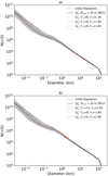 |
Fig. 7 Cumulative SFD for runs corresponding to case 2, using the scaling law showed in Figs. 4a and 4b. The fke function is determined by fke0 = 0.090, γ = 0.5, and β = 0.010. The solid black line is the evolved cumulative SFD from Marschall et al. (2022) for a visual comparison. |
KS test statistics between M22 and ALICANDEP-JT for case 1.
KS test statistics between M22 and ALICANDEP-JT for case 2.
3.3.2 Case 2: Unconventional scaling law (Dmin = 20 m)
The unconventional ![Mathematical equation: $\[Q_{D}^{*}\]$](/articles/aa/full_html/2025/09/aa54339-25/aa54339-25-eq125.png) can be produced by replacing parameters A, a, B and b in Eq. (14) by 7.65 × 105 erg g−1, −0.36, 1.40 erg cm3 g−2 and 1.36, respectively (Marschall et al. 2022). The same scaling law can be written as Eq. (16), using 1.55, 0.36, 24 and 1.71 in place of C1, λ1, C2 and λ2, respectively. In this case, parameter
can be produced by replacing parameters A, a, B and b in Eq. (14) by 7.65 × 105 erg g−1, −0.36, 1.40 erg cm3 g−2 and 1.36, respectively (Marschall et al. 2022). The same scaling law can be written as Eq. (16), using 1.55, 0.36, 24 and 1.71 in place of C1, λ1, C2 and λ2, respectively. In this case, parameter ![Mathematical equation: $\[C_{2}^{\prime}\]$](/articles/aa/full_html/2025/09/aa54339-25/aa54339-25-eq126.png) is tested for values ranging from 4 to 12 combined with
is tested for values ranging from 4 to 12 combined with ![Mathematical equation: $\[\lambda_{2}^{\prime}\]$](/articles/aa/full_html/2025/09/aa54339-25/aa54339-25-eq127.png) , ranging from 1.40 to 1.80, in Eq. (16). The constant values for the fke function are fke0 = 0.090, γ = 0.5 and β = 0.010, which correspond to the best combination for this scaling law that matches the reference run from M22 (Appendix B shows the results for all different parameter combinations of Table 2).
, ranging from 1.40 to 1.80, in Eq. (16). The constant values for the fke function are fke0 = 0.090, γ = 0.5 and β = 0.010, which correspond to the best combination for this scaling law that matches the reference run from M22 (Appendix B shows the results for all different parameter combinations of Table 2).
The statistical analysis presented in Table 4 includes D and p-values for all explored cases. The results reveal a significant similarity between the cumulative distributions obtained with ALICANDEP-JT and M22 considering their unconventional scaling law. Figure 7 shows the evolved SFDs under the ![Mathematical equation: $\[Q_{S}^{*}\]$](/articles/aa/full_html/2025/09/aa54339-25/aa54339-25-eq128.png) scaling laws shown in Figure 4.
scaling laws shown in Figure 4.
The analysis of Figure 7 provides insights into the impact of the scaling law ![Mathematical equation: $\[C_{2}^{\prime}\]$](/articles/aa/full_html/2025/09/aa54339-25/aa54339-25-eq129.png) and
and ![Mathematical equation: $\[\lambda_{2}^{\prime}\]$](/articles/aa/full_html/2025/09/aa54339-25/aa54339-25-eq130.png) parameters on the resulting cumulative SFDs. Specifically, Figure 7b shows that increasing
parameters on the resulting cumulative SFDs. Specifically, Figure 7b shows that increasing ![Mathematical equation: $\[C_{2}^{\prime}\]$](/articles/aa/full_html/2025/09/aa54339-25/aa54339-25-eq131.png) (while keeping
(while keeping ![Mathematical equation: $\[\lambda_{2}^{\prime}\]$](/articles/aa/full_html/2025/09/aa54339-25/aa54339-25-eq132.png) constant) enhances the production of fragments in the 0.1–1 km range, aligning our modelled SFD more closely with the reference distribution in M22. However, this adjustment also leads to a slight overabundance of bodies relative to the initial distribution, particularly near 1 km. This feature, a direct consequence of the unconventional scaling law applied, was also observed by M22 and attributed to the limited yet non-negligible fragmentation of bodies larger than 10 km. Notably, the extreme case tested with
constant) enhances the production of fragments in the 0.1–1 km range, aligning our modelled SFD more closely with the reference distribution in M22. However, this adjustment also leads to a slight overabundance of bodies relative to the initial distribution, particularly near 1 km. This feature, a direct consequence of the unconventional scaling law applied, was also observed by M22 and attributed to the limited yet non-negligible fragmentation of bodies larger than 10 km. Notably, the extreme case tested with ![Mathematical equation: $\[C_{2}^{\prime}\]$](/articles/aa/full_html/2025/09/aa54339-25/aa54339-25-eq133.png) = 4 exhibits significant deviations from the reference run provided by R. Marschall. Overall, our model is consistent with the results of M22, with a preference for
= 4 exhibits significant deviations from the reference run provided by R. Marschall. Overall, our model is consistent with the results of M22, with a preference for ![Mathematical equation: $\[C_{2}^{\prime}\]$](/articles/aa/full_html/2025/09/aa54339-25/aa54339-25-eq134.png) = 8 and
= 8 and ![Mathematical equation: $\[\lambda_{2}^{\prime}\]$](/articles/aa/full_html/2025/09/aa54339-25/aa54339-25-eq135.png) = 1.80.
= 1.80.
4 Results
As outlined in the introduction, the simulations of this section build upon recent work (B25), which successfully modelled the debiased SFD of the hot and cold populations within the Kuiper Belt. That study encompassed several key components, described below.
The SFD of the primordial outer belt is given by:
![Mathematical equation: $\[\begin{aligned}N\left(<H_r\right)= & N_{0_1} 10^{\alpha_s\left(H_r-H_o\right)} \exp \left[-10^{\beta\left(H_r-H_B\right)}\right] \\& +N_{0_2} 10^{\alpha_l\left(H_r-H_o\right)},\end{aligned}\]$](/articles/aa/full_html/2025/09/aa54339-25/aa54339-25-eq138.png) (22)
(22)
where N01 and N02 are constant values. For the parameter values, they followed Petit et al. (2023) using H0 = −2.6, β = 0.25, and HB = 8.1. They assumed a representative albedo of the hot population within the Kuiper belt of pr = 0.08 and a shallow power law slope (αl = 0.18) for large bodies. Furthermore, the slope of small bodies was examined under two distinct values; in case A, a steep slope was considered, αS = 0.4, whereas in case B, a shallower slope was chosen, αS = 0.3. They examined three scaling laws: the nominal one determined by the optimal parameters identified for the unconventional scaling law in Section 3.3.2, and two variations of this scaled by factors of 0.1 and 10 (see Fig. 8). A Maxwellian distribution for impact velocities and different timings for the onset of the giant planets instability (ti) were used.
In the present work, we modelled the collisional evolution of JTs using ALICANDEP-JT with boundary conditions corresponding to each run in B25. Given the negligible exchange of bodies between the two swarms of JTs and the absence of significant collisional interactions, the modelling process was focussed on the most densely populated group, namely, the L4 swarm. The key inputs for the corresponding numerical simulations are as follows.
Initial SFD: the initial size-frequency distribution was set as a fraction of the evolved population of the outer trans-Neptunian disc. Here, we relied on the assumption that since the capture process is size-independent, the captured JT population would be expected to maintain the same SFD shape as the evolved outer belt population at the onset of instability. Consequently, we normalised the whole SFD based on the number of bodies in the size bin corresponding to ~200 km, approximately the largest size for the JT population. This operation leads to a capture probability of 6.5 × 10⁻⁷, which falls within the uncertainties of the jump capture probability of (5 ± 3) × 10−7 estimated by Nesvorný et al. (2013). Thus, the initial SFD preserves all the features of the evolved outer belt at the time of dynamical instability, since the probability of capture at any size is the same. Through this procedure, the resulting total mass of the JT population is about 3 × 10⁻⁶ M⊕, slightly different depending on the specific initial SFD conditions. We note that we performed runs starting with an initial population refereed as case A (αS = 0.4) and case B (αS = 0.3). It is worth noting that the timing of the onset of the instability in the primordial outer belt is of little relevance to the evolution of JTs. This is a consequence of the relatively low-intensity collisional evolution in the primordial disc (B25). For the modelling in this study, we considered the onset of the giant planet instability to take place at ti = 20 Myr.
Scaling law: the same three scaling laws used for the primordial outer belt were also used here (see Fig. 8).
Relative speed and impact probability: The most probable relative speed in the Maxwellian distribution for impact velocities is 4.6 km/s, and the intrinsic impact probability of 7 × 10⁻¹⁸ km−2 yr−1 are adopted, in agreement with previous estimations (Dell’Oro & Paolicchi 1998; Marschall et al. 2022).
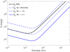 |
Fig. 8 Scaling laws tested for the collisional evolution of JTs. As reference, the solid black line represents the unconventional scaling law |
![Mathematical equation: $\[Q_{D}^{*}\]$](/articles/aa/full_html/2025/09/aa54339-25/aa54339-25-eq136.png)
![Mathematical equation: $\[Q_{S}^{*}\]$](/articles/aa/full_html/2025/09/aa54339-25/aa54339-25-eq137.png)
4.1 Final size-frequency distribution
Figure 9 shows the initial and final cumulative SFDs for the captured population evolved under cases A and B. Each panel shows the results for each tested scaling law. Solid lines show the final cumulative distribution after ~4500 Myr of evolution. The black line shows the observed cumulative SFD for the L4 swarm constructed using the data from the Minor Planet Center1 and the grey dashed line is the observed cumulative SFD for the L4 swarm constructed from Wong & Brown (2015). The size distributions were derived from absolute magnitude (H) data using the standard relationship (Pravec & Harris 2007) as
![Mathematical equation: $\[D=\frac{1329 \times 10^{-H / 5}}{\sqrt{p_V}},\]$](/articles/aa/full_html/2025/09/aa54339-25/aa54339-25-eq139.png) (23)
(23)
where D is the diameter in kilometres and pV is the geometric albedo in the V band. Moving from absolute magnitudes to diameters may introduce significant uncertainties, as real objects have a range of albedo values (Grav et al. 2012). This introduces systematic uncertainties into size estimates based solely on photometric data. For this calculation, we adopted an average geometric albedo of pV = 0.07 for JTs larger than approximately 10 km, as estimated by Grav et al. (2011).
A noticeable gap emerges between the SFDs evolved from the two different αS slope values (referred to as cases A and B). Using the same scaling law, case A (αS = 0.4) keeps its steep SFD that persists over the observed distribution. On the contrary, case B, corresponding to a shallower slope (αS = 0.3), underestimates the population, particularly at sizes smaller than ~20 km. This finding is consistent with the conclusions by B25, who determined that a slope of αS = 0.4 in the outer primordial distribution achieves an excellent match with the de-biased populations of the Kuiper belt.
A common feature of cases A and B is an excess of bodies around 1 km that is not usually observed when traditional scaling laws (which have a minimum at hundreds of kilometres) are applied. This feature is a by-product of the unconventional scaling law used and was also noticed by M22. Here, we see that this feature is more pronounced for runs corresponding to the scaling law for strong bodies, and it is smoothed for the weakest bodies. For instance, Fig. 9a shows an excess of bodies – up to a factor of 2 over the corresponding initial population – in a range spanning up to one order of magnitude around 1 km. This is due to inefficient collisional grinding (in the relatively rarefied JT environment) of newly produced fragments from the disruption and cratering of bodies larger than 10 km.
Focusing on the results of case A, which are more consistent with the observational data, and comparing the final SFD for different scaling laws (represented by the solid blue lines in Figure 9), it is evident that each scaling law produces a distinct shape in the final SFD. Thus, the weaker the scaling law, the smaller the gap between the modelled and the observed JT SFDs. Conversely, decreasing the strength (e.g. to the nominal scaling law, shown in the middle panel) heightens the fragmentation of bodies around 10 km, giving rise to a dip in the SFD in the 5 to ~30 km range. Hence, the evolved SFD approximates the observed distribution in that size range. Notably, the SFD modelled using the scaling law that represents the weakest bodies (bottom panel) aligns even more closely with the observed SFD. This is due to the fragility of bodies, which allow for fragmentation up to ~100 km, thereby increasing the depth of the dip, which in this case extends up to ~60 km. Consequently, the scaling law SL1 × 0.1, combined with a suitable initial SFD (αS = 0.4), matches the observed cumulative size distribution of JT above the completeness limit (~10 km).
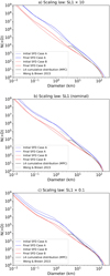 |
Fig. 9 Initial (dashed lines) and final (solid lines) cumulative SFDs of the modelled JT population from each scaling law shown in Fig. 8. Blue and red lines correspond to cases A and B, corresponding to αS = 0.4 and αS = 0.3, respectively. The black solid line represents the cumulative SFD of data from the Minor Planet Center for the L4 swarm, and the dashed gray line corresponds to the SFD estimated by Wong & Brown (2015), including an extrapolation to smaller sizes. |
4.2 Collisional families
An additional way to constrain our modelling results is by comparing the number of collisional families whose parent bodies were larger than ~100 km. This provides a valuable observational constraint, as only a few such large families are currently identified among the JTs. Based on a detailed analysis of the trojan population, Vokrouhlický et al. (2024) identified three to five families whose parent bodies likely exceeded 100 km in diameter, using the methodology of Durda et al. (2007) to estimate progenitor sizes. This range offers a useful benchmark to test our collisional evolution model. In our best-case scenario (SL1×0.1, case A), the initial SFD has 17 bodies with diameters larger than D ~ 90 km. After ~4.5 Gyr of evolution, five of them underwent catastrophic disruption: three with D ~ 95 km and two with D ~ 120 km. While the diameters of our disrupted bodies are somewhat smaller than those reported by Vokrouhlický et al. (2024), the agreement is overall satisfactory, especially considering the different approaches used to define parent body sizes. Our results are therefore consistent with the observed number of large trojan families and support the validity of the size distribution and collisional parameters adopted in our model. This supports the ‘weak’ scaling law as the most suitable one for modelling the evolution of the JTs.
4.3 Comparison with the colour sub-populations of JTs
The bimodal colour distribution observed among JTs has been interpreted as evidence of two distinct subpopulations: a red (R) group, considered to be the remnant of the captured primordial bodies, and a less red (LR) group, proposed to consist mainly of fragments produced through collisional evolution after emplacement in the region. This hypothesis, widely discussed in Wong & Brown (2015); Wong & Brown (2017), is supported by the different SFDs observed for the two colour groups. In particular, the LR population exhibits a significantly steeper slope and becomes dominant at smaller sizes, whereas the R population follows a broken power-law SFD consistent with a preserved primordial distribution at large sizes. In this framework, collisions play a crucial role in shaping the present-day colour and size distribution of the trojan population, suggesting that the surface properties of small objects are largely determined by collisional processing. To test the consistency of this scenario with our collisional evolution models, we made use of a tool in our code that allows us to track the number of primordial bodies throughout the evolution. We applied this tool to our reference case (SL1×0.1, case A) and examined the SFD of the total evolved population, the remaining primordial objects, and the collisional fragments produced by the evolution. The results are presented in Fig. 10. The initial SFD, which resembles that of the trans-Neptunian source region at the time of capture, is shown as a black dashed line. The solid black line shows the total population at the end of the simulation. The remnant primordial bodies, corresponding to the R population, are plotted by a dashed red line, while the fragments (interpreted as the LR population) are shown by a solid blue line. As expected, the primordial population remains largely unaltered at large sizes (D > 70 km) but becomes strongly depleted below a few kilometres. In contrast, the fragment population follows a steep slope down to small sizes and begins to dominate the total SFD around D ~ 14 km. This behaviour is in good agreement with the observed trends for the LR population described by Wong & Brown (2015).
Such results provide quantitative support for the hypothesis that the colour bimodality of JTs reflects their collisional history. The R and LR groups, as defined spectrally, can be naturally mapped onto categories of primordial bodies and collisional fragments, respectively, in our model. The fact that the transition between R- and LR-dominated regimes occurs around ~14 km and that the LR population dominates entirely below a few kilometres strengthens the view that small trojans are primarily produced when their parent bodies are located in the L4 trojan region.
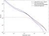 |
Fig. 10 SFDs from our best case run (SL1×0.1, case A). The black dashed line shows the initial SFD of the primordial population at the time of JT emplacement. The solid black line corresponds to the total evolved population after 4 Gyr of collisional evolution. The red line represents the remnant primordial population, while the blue line shows the population of fragments produced during collisions. |
4.4 Expected craters SFD of Lucy Mission targets
This section presents the predicted crater size distribution for the Lucy mission targets at the equilibrium point L4 corresponding to the evolution conditions that better match the observed JT SFD, as shown in Sect. 4.1 (case A and SL1 × 0.1). To provide context, we begin by briefly describing the key characteristics of (15094) Polymele, (11351) Leucus, (21900) Orus, and (3548) Eurybates. Afterwards, we introduce the cratering law used in this work and present results for the cratering record on the mentioned targets.
4.4.1 Lucy Mission targets in the L4 swarm
(15094) Polymele is the smallest Lucy target in L4 and it probably has an ellipsoidal shape (Levison et al. 2023). Its estimated effective diameter is 21 km, with a rotational period of ~11.5 h (Levison et al. 2021). It is a dark, reddish, and P-type asteroid. Stellar occultations revealed that Polymele is accompanied by a small satellite tentatively named Shaun, about 5–6 km in diameter (Buie et al. 2022).
(11351) Leucus exhibits interesting features, as revealed by stellar occultations (Buie et al. 2021). This trojan slow rotator appears to have an elongated, prolate shape with approximate sizes 63.8 × 36.6 × 14.8 km, corresponding to an equivalent spherical diameter of 41 km. Lucus is a D-type asteroid with a very dark surface and apparently significant topographic features that may suggest a complex collisional history.
(21900) Orus photometric observations and stellar occultations revealed updated features of this asteroid (Mottola et al. 2023; Buie et al. 2020). Orus D-type asteroid has a retrograde spin with a sidereal rotation period of 13.486 hours, as determined from photometric light-curve observations (Mottola et al. 2023). Stellar occultation data suggest a surface-equivalent spherical diameter of 60.5 ± 0.96 km. Orus is characterised by its very red colour and it appears to have a convex shape, indicative of its surface morphology and potential collisional history.
(3548) Eurybates photometric observations and stellar occultations provided refined details about this asteroid (Mottola et al. 2023; Buie et al. 2020). This C-type JT has a retrograde spin with a sidereal rotation period of 8.73 h, as determined from photometric light curve observations. Stellar occultation data estimate its surface-equivalent spherical diameter as 69.3 ± 1.4 km. As the largest member of the Eurybates collisional family, it apparently has a convex shape. Additionally, the Hubble Space Telescope identified a 1-km satellite orbiting Eurybates (Noll et al. 2020), likely a remnant of its collisional history.
4.4.2 Cratering scaling law
To estimate any cumulative crater size distribution, we need to calculate the transient crater diameter (Dt) caused by a projectile with size d and the corresponding final crater size (Dc). The Pi-group scaling law formulation provided by Holsapple & Housen (2007) allows us to obtain Dt as a function of the impact conditions and material properties. After the collapse of the transient crater, the final crater is usually estimated as Dc = λDt (λ ≥ 1 is determined empirically). In fact, in the cratering process, immediately after the crater excavation, a transient crater is formed. Afterwards, the outer structure collapses due to gravity, and the crater is ultimately modified to its final form; the resulting crater is wider than its transient form. Typical values for λ are usually assumed to be in the range 1.2–1.5. Thus, the following relationship allows for the calculation of the diameter of the crater produced by any specific collision.
![Mathematical equation: $\[D_c=\lambda k_1 d\left[\frac{g d}{2 V_P^2}\left(\frac{\rho}{\delta}\right)^{\frac{2 \nu}{\mu}}+k_2\left(\frac{Y}{\rho V_P^2}\right)^{\frac{2+\mu}{2}}\left(\frac{\rho}{\delta}\right)^{\frac{\nu(2+\mu)}{\mu}}\right]^{-\frac{\mu}{2+\mu}},\]$](/articles/aa/full_html/2025/09/aa54339-25/aa54339-25-eq140.png) (24)
(24)
where VP is the projectile velocity component perpendicular to the surface, δ is the bulk density, Y is the strength of the target material, k1, k2, μ, and ν account for the nature of the target terrain. Finally, g = (4/3) (D/2) πGρ, is the surface gravity, where D is the diameter of the target, G is the gravitational constant, and ρ is the density of the target, while considering that it is spherical and homogeneous.
The knowledge of some parameters in Eq. (24) is limited, especially regarding the composition of JTs, which are likely a combination of rock and ice (Wong et al. 2014). Then, we need to make some assumptions about material properties. Specifically, we set both the density of the material (ρ) and the bulk density (δ) to 1 g cm−3, consistent with the assumptions of the collisional evolution model. Holsapple & Housen (2007) pointed out that 1/3 < μ < 2/3 (depending on the energy dissipation of the material) and the experimental results suggest that ν ≃ 0.4 for most materials. Consequently, parameters (k1, k2, ν, μ) are assigned suitable values for the target composition of rocks (0.93, 1, 0.4, 0.55) and highly porous materials (0.725, 1, 0.4, 0.4). Finally, the Y parameter remains largely unknown. In this study, we explore a range of strength values for rocky materials: 10 kPa (soft rock) and 1 MPa (hard rock). This choice is justified by the wide range of estimates found in the literature. To provide context for these values, some regions of the lunar regolith have low tensile strengths ranging 1–12 kPa (Slyuta 2014; Ding et al. 2024), while harder rock materials can reach strengths in the 10–18 MPa range (Holsapple 1993). Additionally, for highly porous materials, we assumed 10 kPa.
4.4.3 Cratering record
Here, we present the results for the Lucy targets located in L4, showing the cumulative number of craters per unit area (Nc(> D) [km−2]) as a function of crater size. Normalization to the unit area is achieved by calculating the surface area of each body, considered as a sphere of radius equal to its equivalent radius. The effective diameter of each target were taken from Table 3 in Levison et al. (2021). The figures in this section show the outcome corresponding to our preferred parameter choice discussed in Section 4.1 (case A and SL1 × 0.1), for the two tested cratering scaling laws: rock and highly porous material, as specified earlier in this paper.
Figure 11 presents the cumulative crater distribution for the four targets. As expected, all targets follow a similar trend for small craters. However, noticeable differences arise for large craters due to the dependence of crater size on Y and μ in Eq. (24), which governs the transition between strength– and gravity–dominated regimes. For rocky targets, the influence of the strength parameter is particularly evident. Increasing the material strength by a factor of two not only reduces the overall crater size but also extends the range of large craters across different target sizes. In the case of low-strength material (Y = 10 kPa), the surface may become fully saturated with small craters (<0.2 km) and are more than 10% saturated for large craters. Conversely, for high-strength material (Y = 1 MPa), the surface may have significant crater deficiency at all size ranges. Notably, the cratering scaling law for hard rock produces a crater size distribution similar to porous targets with Y = 10 kPa.
Those results highlight the critical role of material properties in shaping the expected crater size distribution on JT surfaces. To explore this further, we focus on Eurybates and apply a cratering scaling law previously used for the icy surfaces of small and mid-sized Saturnian satellites, characterised by (κ1, κ2, ν, μ) = (1.67, 0.351, 0.397, 0.38) and Y = 15 kPa (Di Sisto & Zanardi 2013; Rossignoli et al. 2019). As shown in Figure 12, if JTs have icy compositions, their surfaces may reach approximately 10% saturation for craters in the ~1–5 km size range, with even higher saturation levels at both small and large craters.
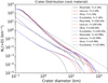 |
Fig. 11 Cumulative number of craters per unit surface, on (15094) Polymele, (11351) Leucus, (21900) Orus and (3548) Eurybates. Results gathered from a run under case A (αS = 0.4). The parameter for rocky material are (κ1, κ2, ν, μ)=(0.93,1,0.4,0.55), using Y=10 kPa for soft rock (dashed lines) and Y=1 MPa for hard rock (solid lines). The parameter for porous material are (κ1, κ2, ν, μ)=(0.725,1,0.4,0.4) (dotted lines), grey lines indicate crater saturation levels, with a dashed line indicating 10% and a dotted line 100% of geometric saturation. |
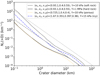 |
Fig. 12 Cumulative number of craters per unit surface area on (3548) Eurybates testing different materials, as indicated in the legend. Results are obtained from a run under case A (αS = 0.4), gray lines indicate crater saturation levels, with the dashed line indicating 10% and the dotted line full (100%) of geometric saturation. |
5 Summary and conclusions
In this study, we examine the collisional evolution of the JTs population using a customised version of ALICANDEP called ALICANDEP-JT. Our investigation involves a comprehensive comparison with established models, such as those proposed by de Elía & Brunini (2007) and Marschall et al. (2022), enabling us to both validate our model and explore the relationship between shattering and disruption threshold specific energy. Following the validation and determination of suitable values for the parameters in the shattering scaling laws, we employed our code package to model the collisional evolution of JT under the capture hypothesis. We used an initial SFD derived from recent studies (B25) on the collisional evolution of the primordial trans-Neptunian disc as a baseline. The key findings of this study are as follows.
Code validation and link between
![Mathematical equation: $\[Q_{D}^{*}\]$](/articles/aa/full_html/2025/09/aa54339-25/aa54339-25-eq141.png) and
and ![Mathematical equation: $\[Q_{S}^{*}\]$](/articles/aa/full_html/2025/09/aa54339-25/aa54339-25-eq142.png) : Overall, our comparison of ALICANDEP-JT with previous research yielded positive results. First, we showed that our model can reproduce similar outcomes to de Elía & Brunini (2007), under equivalent fragmentation model and evolutionary conditions. Furthermore, we compared our model with the evolved SFD obtained by Marschall et al. (2022) using the Boulder code. The main difference between the two models is that the Boulder code does not deal with the fragmentation and re-accumulation process; instead, it directly includes the results of previous collision modelling via SPH codes and scales the fragment distribution accordingly. A satisfactory agreement between the two models was achieved for the considered cases, establishing a link between
: Overall, our comparison of ALICANDEP-JT with previous research yielded positive results. First, we showed that our model can reproduce similar outcomes to de Elía & Brunini (2007), under equivalent fragmentation model and evolutionary conditions. Furthermore, we compared our model with the evolved SFD obtained by Marschall et al. (2022) using the Boulder code. The main difference between the two models is that the Boulder code does not deal with the fragmentation and re-accumulation process; instead, it directly includes the results of previous collision modelling via SPH codes and scales the fragment distribution accordingly. A satisfactory agreement between the two models was achieved for the considered cases, establishing a link between ![Mathematical equation: $\[Q_{D}^{*}\]$](/articles/aa/full_html/2025/09/aa54339-25/aa54339-25-eq143.png) and
and ![Mathematical equation: $\[Q_{S}^{*}\]$](/articles/aa/full_html/2025/09/aa54339-25/aa54339-25-eq144.png) under consistent conditions for the re-accumulation model and the fke parameter. The plots in Appendix A highlight the need of including a constant β in the fke function to improve the match with M22 in the size range from 100 m to a few kilometres, especially in the case the scaling law has a minimum at 250 m. Our analysis revealed that the location of the minimum in
under consistent conditions for the re-accumulation model and the fke parameter. The plots in Appendix A highlight the need of including a constant β in the fke function to improve the match with M22 in the size range from 100 m to a few kilometres, especially in the case the scaling law has a minimum at 250 m. Our analysis revealed that the location of the minimum in ![Mathematical equation: $\[Q_{S}^{*}\]$](/articles/aa/full_html/2025/09/aa54339-25/aa54339-25-eq145.png) is shifted by a factor of 2 toward large sizes, compared to the corresponding
is shifted by a factor of 2 toward large sizes, compared to the corresponding ![Mathematical equation: $\[Q_{D}^{*}\]$](/articles/aa/full_html/2025/09/aa54339-25/aa54339-25-eq146.png) minimum.
minimum.-
Collisional evolution of JT under the capture scenario: Our findings support the hypothesis that JTs originated in the outer disc, before being captured by Jupiter during the instability phase of the giant planets. To model this scenario, we picked a fraction of the evolved outer population at the onset of the instability period, and let it evolve collisionally under the JT boundary conditions. Such fraction corresponds to a capture probability of 6.5 × 10⁻⁷, which is consistent with the capture probability of (5 ± 3) × 10−7 estimated by Nesvorný et al. (2013). The optimal agreement between the modelled SFDs of JTs after 4500 Myr and the observed population within the L4 swarm allowed us to identify the most suitable scaling law governing the fragmentation process and the preferred slope of the SFD at the small-size end, for the primordial outer population. Our analysis revealed that weak bodies necessarily underwent collisional grinding to match the observed JT SFDs closely. Furthermore, we determined that only a primordial population with a steep slope of the cumulative magnitude distribution (α = 0.4) can accurately reproduce the observed SFD of JTs. These results support the match between the B25 findings and the present-day debiased Kuiper Belt populations. This study shows that the JT underwent a more intense collisional evolution than Kuiper Belt objects. Such a collisional process modified the JT SFD, giving it a more pronounced wave-like structure than the one left in the outer belt by collisional processes during the pre-instability phase.
Although our findings are in promising agreement with the observed JT population, we acknowledge that other possible combinations of parameters (within limits) may also yield satisfactory results. Multiple factors may cause such a degeneracy. For instance, to build the observed SFD, one needs to make assumptions, for instance, for the mean albedo value. Several intrinsic parameters related to the fragmentation and evolution processes must also be assumed in the numerical modelling, such as the bulk density, impact speed distribution, intrinsic impact probability, and so on (even if for many of these, enough information is already available to reduce the degeneracy).
Collisional families: among all the simulations performed, only our best-fit scenario (SL1 × 0.1, case A) reproduced the observed number of large collisional families. In this case, five parent bodies with diameters above 90 km underwent catastrophic disruption over 4.5 Gyr. This is in good agreement with the three to five families inferred from the current trojan population (Vokrouhlický et al. 2024). This outcome further supports the plausibility of the SL1 × 0.1 configuration as the most realistic scenario explored in this work.
Colour sub-populations. Our modelling supports the hypothesis proposed by Wong & Brown (2015); Wong & Brown (2017) that the observed colour bimodality among JTs reflects their collisional evolution. By tracking the primordial and fragment populations separately, we show that the less red (LR) component (interpreted as collisional fragments) follows a steep size-frequency distribution and becomes dominant below ≈14 km in diameter. Conversely, the red (R) component – related to primordial bodies – retains the shape of the initial SFD at large sizes and becomes progressively depleted below a few kilometre sizes due to disruptive collisions. This dual behaviour reproduces the main observational trends and reinforces the interpretation that the R population traces the original captured bodies, while the LR population is largely the result of subsequent collisional processing.
-
Cratering records: after our code was validated and the collisional evolution of JT was explored under the capture hypothesis, the ALICANDEP-JT package was used to make predictions about the surface characteristics of the objects that will be visited by the Lucy spacecraft in the L4 swarm. Specifically, we analysed the crater distribution on bodies of sizes comparable to Lucy’s targets. For rocky JTs, low-strength materials (soft rock, Y = 10 kPa) result in a geometric saturation larger than 10%. In contrast, high-strength materials (hard rock, Y = 10 MPa) lead to crater-deficient surfaces. For porous materials, the crater distribution is similar to that of hard rock, while icy compositions imply a distribution that falls between soft and hard rock, reaching a geometric saturation close to 10%.
Further analyses of Eurybates show that changes in the cratering scaling law parameters, such as μ and k, produce different features in the crater size distribution. Such findings emphasize the need for precise knowledge of the surface composition properties to accurately constrain the population of small JTs from the cratering record, ensuring a proper interpretation of Lucy’s mission data.
Former studies of the cratering records on JT Lucy targets, such as that of Marchi et al. (2023), have provided valuable information. The parameter sets chosen by Marchi et al. (2023) to represent cohesive soils and porous bodies produce distributions that are relatively similar to each other. Nevertheless, they seem to overlook the substantial variability introduced by significant uncertainties on critical parameter values for the cratering scaling laws. In the present work, we tried to cover this issue by introducing a comprehensive exploration of the parameter space, crucial for capturing the diversity of surface properties of JTs.
Acknowledgements
We thank Raphael Marschall for kindly providing the SFDs from his work, and Romina Di Sisto for her helpful suggestions. PGB and ACB acknowledge support from the Generalitat Valenciana through grant CIAICO/2021/328. PGB also acknowledges funding from the European Space Agency under the Science Faculty program (Funding reference ESA-SCI-SC-LE-191). VSC thanks the University of Coimbra for supporting his stay at the University of Alicante through the Erasmus+ program. TSR acknowledges funding from Ministerio de Ciencia e Innovación (Spanish Government), PGC2021, PID2021-125883NB-C21. This work was (partially) supported by the Spanish MICIN/AEI/10.13039/501100011033 and by ‘ERDF A way of making Europe’ by the ‘European Union’ through grant PID2021-122842OB-C21, and the Institute of Cosmos Sciences University of Barcelona (ICCUB, Unidad de Excelencia ‘María de Maeztu’) through grant CEX2019-000918-M. We also thank reviewer Vokrouhlický for helpful suggestions on the submitted manuscript.
References
- Benavidez, P. G., & Campo Bagatin, A. 2009, Planet. Space Sci., 57, 201 [Google Scholar]
- Benavidez, P., Campo Bagatin, A., Serra Cardoso, V., & Santana-Ros, T. 2025, Nat. Comm., submitted [Google Scholar]
- Benz, W., & Asphaug, E. 1999, Icarus, 142, 5 [NASA ADS] [CrossRef] [Google Scholar]
- Bottke, W. F., Durda, D. D., Nesvorný, D., et al. 2005, Icarus, 175, 111 [Google Scholar]
- Bottke, W. F., Marschall, R., Nesvorný, D., & Vokrouhlický, D. 2023a, Space Sci. Rev., 219, 83 [Google Scholar]
- Bottke, W. F., Vokrouhlický, D., Marshall, R., et al. 2023b, PSJ, 4, 168 [Google Scholar]
- Bottke, W. F., Vokrouhlický, D., Nesvorný, D., et al. 2024, PSJ, 5, 88 [Google Scholar]
- Buie, M. W., Keeney, B., Levison, H., et al. 2020, in AAS/Division for Planetary Sciences Meeting Abstracts, 52, 401.02 [Google Scholar]
- Buie, M. W., Keeney, B. A., Strauss, R. H., et al. 2021, PSJ, 2, 202 [Google Scholar]
- Buie, M., Keeney, B., Levison, H., Olkin, C., & Lucy Occultations Team. 2022, in AAS/Division for Planetary Sciences Meeting Abstracts, 54, 512.03 [Google Scholar]
- Campo Bagatin, A., & Benavidez, P. G. 2012, MNRAS, 423, 1254 [NASA ADS] [CrossRef] [Google Scholar]
- Campo Bagatin, A., Cellino, A., Davis, D. R., Farinella, P., & Paolicchi, P. 1994, Planet. Space Sci., 42, 1079 [NASA ADS] [CrossRef] [Google Scholar]
- Campo Bagatin, A., Petit, J.-M., & Farinella, P. 2001, Icarus, 149, 198 [Google Scholar]
- Davis, D. R., Chapman, C. R., Weidenschilling, S. J., & Greenberg, R. 1985, Icarus, 62, 30 [NASA ADS] [CrossRef] [Google Scholar]
- Davis, D. R., Weidenschilling, S. J., Farinella, P., Paolicchi, P., & Binzel, R. P. 1989, in Asteroids II, eds. R. P. Binzel, T. Gehrels, & M. S. Matthews (Tucson, USA: University of Arizona Press), 805 [Google Scholar]
- Davis, D. R., Durda, D. D., Marzari, F., Campo Bagatin, A., & Gil-Hutton, R. 2002, in Asteroids III, eds. W. F. Bottke, A. Cellino, P. Paolicchi, & R. P. Binzel (Tucson, USA: University of Arizona Press), 545 [Google Scholar]
- de Elía, G. C., & Brunini, A. 2007, A&A, 475, 375 [NASA ADS] [CrossRef] [EDP Sciences] [Google Scholar]
- Dell’Oro, A., & Paolicchi, P. 1998, Icarus, 136, 328 [Google Scholar]
- Dell’Oro, A., Marzari, F., Paolicchi, P., & Vanzani, V. 2001, A&A, 366, 1053 [CrossRef] [EDP Sciences] [Google Scholar]
- Di Sisto, R. P., & Zanardi, M. 2013, A&A, 553, A79 [NASA ADS] [EDP Sciences] [Google Scholar]
- Ding, L., Zhou, R., Yu, T., et al. 2024, Nat. Commun., 15, 2098 [Google Scholar]
- Durda, D. D., Bottke, W. F., Nesvorný, D., et al. 2007, Icarus, 186, 498 [NASA ADS] [CrossRef] [Google Scholar]
- Emery, J. P., Marzari, F., Morbidelli, A., French, L. M., & Grav, T. 2015, in Asteroids IV, eds. P. Michel, F. E. DeMeo, & W. F. Bottke (Tucson, USA: University of Arizona Press), 203 [Google Scholar]
- Fujiwara, A., Kamimoto, G., & Tsukamoto, A. 1977, Icarus, 31, 277 [NASA ADS] [CrossRef] [Google Scholar]
- Gault, D. E., Moore, H. J., & Shoemaker, E. M. 1963, Crater Size Distributions and Impact Velocities, Tech. Rep. NASA-TN-D-1767, NASA [Google Scholar]
- Giblin, I., Davis, D. R., & Ryan, E. V. 2004, Icarus, 171, 487 [Google Scholar]
- Grav, T., Mainzer, A. K., Bauer, J., et al. 2011, ApJ, 742, 40 [NASA ADS] [CrossRef] [Google Scholar]
- Grav, T., Mainzer, A. K., Bauer, J. M., Masiero, J. R., & Nugent, C. R. 2012, ApJ, 759, 49 [NASA ADS] [CrossRef] [Google Scholar]
- Holsapple, K. A. 1993, Annu. Rev. Earth Planet. Sci., 21, 333 [CrossRef] [Google Scholar]
- Holsapple, K. A., & Housen, K. R. 2007, Icarus, 187, 345 [NASA ADS] [CrossRef] [Google Scholar]
- Housen, K. R., & Holsapple, K. A. 1990, Icarus, 84, 226 [NASA ADS] [CrossRef] [Google Scholar]
- Kavelaars, J. J., Petit, J.-M., Gladman, B., et al. 2021, ApJ, 920, L28 [NASA ADS] [CrossRef] [Google Scholar]
- Levison, H. F., Olkin, C. B., Noll, K. S., et al. 2021, PSJ, 2, 171 [Google Scholar]
- Levison, H., Buie, M., Keeney, B., & Mottola, S. 2023, in AAS/Division for Planetary Sciences Meeting Abstracts, 55, 107.05 [Google Scholar]
- Lyra, W., Johansen, A., Cañas, M. H., & Yang, C.-C. 2023, ApJ, 946, 60 [CrossRef] [Google Scholar]
- Marchi, S., Nesvorný, D., Vokrouhlický, D., Bottke, W. F., & Levison, H. 2023, AJ, 166, 221 [Google Scholar]
- Marschall, R., Nesvorný, D., Deienno, R., et al. 2022, AJ, 164, 167 [NASA ADS] [CrossRef] [Google Scholar]
- Marzari, F., Farinella, P., & Vanzani, V. 1995, A&A, 299, 267 [NASA ADS] [Google Scholar]
- Marzari, F., Farinella, P., Davis, D. R., Scholl, H., & Campo Bagatin, A. 1997, Icarus, 125, 39 [Google Scholar]
- Melosh, H. J. 1989, Impact Cratering: A Geologic Process (Oxford University Press), 254 [Google Scholar]
- Melosh, H. J., & Ryan, E. V. 1997, Icarus, 129, 562 [Google Scholar]
- Morbidelli, A., & Nesvorný, D. 2020, The Primordial Sculpting of the Main Belt (Elsevier), 25 [Google Scholar]
- Morbidelli, A., Levison, H. F., Tsiganis, K., & Gomes, R. 2005, Nature, 435, 462 [Google Scholar]
- Morbidelli, A., Bottke, W. F., Nesvorný, D., & Levison, H. F. 2009, Icarus, 204, 558 [Google Scholar]
- Mottola, S., Hellmich, S., Buie, M. W., et al. 2023, PSJ, 4, 18 [Google Scholar]
- Nakamura, A., & Fujiwara, A. 1991, Icarus, 92, 132 [Google Scholar]
- Nesvorný, D., & Morbidelli, A. 2012, AJ, 144, 117 [Google Scholar]
- Nesvorný, D., Vokrouhlický, D., & Morbidelli, A. 2013, ApJ, 768, 45 [CrossRef] [Google Scholar]
- Nesvorný, D., Vokrouhlický, D., Bottke, W. F., & Levison, H. F. 2018, Nat. Astron., 2, 878 [Google Scholar]
- Noll, K. S., Brown, M. E., Weaver, H. A., et al. 2020, PSJ, 1, 44 [NASA ADS] [Google Scholar]
- O’Brien, D. P., & Greenberg, R. 2005, Icarus, 178, 179 [CrossRef] [Google Scholar]
- Petit, J.-M., & Farinella, P. 1993, Celest. Mech. Dyn. Astron., 57, 1 [Google Scholar]
- Petit, J.-M., Gladman, B., Kavelaars, J. J., et al. 2023, ApJ, 947, L4 [NASA ADS] [CrossRef] [Google Scholar]
- Pirani, S., Johansen, A., Bitsch, B., Mustill, A. J., & Turrini, D. 2019a, A&A, 623, A169 [NASA ADS] [CrossRef] [EDP Sciences] [Google Scholar]
- Pirani, S., Johansen, A., & Mustill, A. J. 2019b, A&A, 631, A89 [NASA ADS] [CrossRef] [EDP Sciences] [Google Scholar]
- Pitjeva, E. V., & Pitjev, N. P. 2020, Astron. Lett., 45, 855 [Google Scholar]
- Pravec, P., & Harris, A. W. 2007, Icarus, 190, 250 [CrossRef] [Google Scholar]
- Rossignoli, N. L., Di Sisto, R. P., Zanardi, M., & Dugaro, A. 2019, A&A, 627, A12 [NASA ADS] [CrossRef] [EDP Sciences] [Google Scholar]
- Slyuta, E. N. 2014, Sol. Syst. Res., 48, 330 [Google Scholar]
- Uehata, K., Terai, T., Ohtsuki, K., & Yoshida, F. 2022, AJ, 163, 213 [NASA ADS] [CrossRef] [Google Scholar]
- Vinogradova, T. A., & Chernetenko, Y. A. 2015, Sol. Syst. Res., 49, 391 [Google Scholar]
- Vokrouhlický, D., Nesvorný, D., Brož, M., et al. 2024, AJ, 167, 138 [Google Scholar]
- Vokrouhlický, D., Nesvorný, D., Brož, M., et al. 2025, AJ, 169, 242 [Google Scholar]
- Wong, I., & Brown, M. E. 2015, AJ, 150, 174 [NASA ADS] [CrossRef] [Google Scholar]
- Wong, I., & Brown, M. E. 2017, AJ, 153, 145 [Google Scholar]
- Wong, I., Brown, M. E., & Emery, J. P. 2014, AJ, 148, 112 [Google Scholar]
- Zain, P. S., Di Sisto, R. P., & Gil-Hutton, R. 2025, A&A, 694, A298 [NASA ADS] [CrossRef] [EDP Sciences] [Google Scholar]
Appendix A Testing fke parameters for case 1: Q0 scaling law (Dmin = 250 m)
In this appendix, we show the SFD for various combinations of fke parameters listed in Table 2 for each scaling law refereed as case 1. Figures A.1 and A.2 illustrate that different combinations of ![Mathematical equation: $\[C_{2}^{\prime}\]$](/articles/aa/full_html/2025/09/aa54339-25/aa54339-25-eq147.png) and
and ![Mathematical equation: $\[\lambda_{2}^{\prime}\]$](/articles/aa/full_html/2025/09/aa54339-25/aa54339-25-eq148.png) , with β = 0 in the fke function do not produce a depth as significant as that achieved in the reference run from M22, across the size range of a few meters to several kilometres. However, by assuming a constant value of β = 0.015, our modelled SFDs align closely with the reference SFD from M22 within the same size range (see Figures A.3 and A.4).
, with β = 0 in the fke function do not produce a depth as significant as that achieved in the reference run from M22, across the size range of a few meters to several kilometres. However, by assuming a constant value of β = 0.015, our modelled SFDs align closely with the reference SFD from M22 within the same size range (see Figures A.3 and A.4).
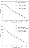 |
Fig. A.1 Evolved SFDs for case 1 (Q0 scaling law with Dmin = 250 m) with parameters indicated in the legend. fke parameters: fke0 = 0.35, γ = 0.7, and β = 0. The black solid line is the reference case of M22. |
Appendix B Testing fke parameters for case 2: Unconventional scaling law (Dmin = 20 m)
Here, we show the SFD for different combinations of fke parameters listed in Table 2 for each scaling law refereed as case 2. Figures B.1, B.2, B.3, and B.4 show that the β value is not very critical when the minimum of the scaling law is at ~20 m.
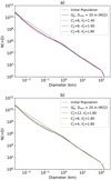 |
Fig. B.1 Evolved SFDs for case 2 (unconventional scaling law with Dmin = 20 m) with parameters indicated in the legend. fke parameters: fke0 = 0.35, γ = 0.7, and β = 0. The black solid line is the reference case of M22. |
All Tables
All Figures
|
Fig. 1 Comparison of two selected scaling laws from EB07, |
| In the text | |
|
Fig. 2 Cumulative SFDs for cases |
| In the text | |
|
Fig. 3
|
| In the text | |
|
Fig. 4
|
| In the text | |
|
Fig. 5 Functions of fke tested and listed in Table 2. Black symbols correspond to values from Nakamura & Fujiwara (1991); Melosh & Ryan (1997); and Giblin et al. (2004), as indicated in the legend. |
| In the text | |
|
Fig. 6 Cumulative SFDs for runs corresponding to case 1, using the scaling laws showed in Figs. 3a and 3b). The fke function is determined by fke0 = 0.085, γ = 0.5 and β = 0.015. The solid black line is the evolved cumulative SFD using the scaling law, Q0, from Marschall et al. (2022) for visual comparison. |
| In the text | |
|
Fig. 7 Cumulative SFD for runs corresponding to case 2, using the scaling law showed in Figs. 4a and 4b. The fke function is determined by fke0 = 0.090, γ = 0.5, and β = 0.010. The solid black line is the evolved cumulative SFD from Marschall et al. (2022) for a visual comparison. |
| In the text | |
|
Fig. 8 Scaling laws tested for the collisional evolution of JTs. As reference, the solid black line represents the unconventional scaling law |
| In the text | |
|
Fig. 9 Initial (dashed lines) and final (solid lines) cumulative SFDs of the modelled JT population from each scaling law shown in Fig. 8. Blue and red lines correspond to cases A and B, corresponding to αS = 0.4 and αS = 0.3, respectively. The black solid line represents the cumulative SFD of data from the Minor Planet Center for the L4 swarm, and the dashed gray line corresponds to the SFD estimated by Wong & Brown (2015), including an extrapolation to smaller sizes. |
| In the text | |
|
Fig. 10 SFDs from our best case run (SL1×0.1, case A). The black dashed line shows the initial SFD of the primordial population at the time of JT emplacement. The solid black line corresponds to the total evolved population after 4 Gyr of collisional evolution. The red line represents the remnant primordial population, while the blue line shows the population of fragments produced during collisions. |
| In the text | |
|
Fig. 11 Cumulative number of craters per unit surface, on (15094) Polymele, (11351) Leucus, (21900) Orus and (3548) Eurybates. Results gathered from a run under case A (αS = 0.4). The parameter for rocky material are (κ1, κ2, ν, μ)=(0.93,1,0.4,0.55), using Y=10 kPa for soft rock (dashed lines) and Y=1 MPa for hard rock (solid lines). The parameter for porous material are (κ1, κ2, ν, μ)=(0.725,1,0.4,0.4) (dotted lines), grey lines indicate crater saturation levels, with a dashed line indicating 10% and a dotted line 100% of geometric saturation. |
| In the text | |
|
Fig. 12 Cumulative number of craters per unit surface area on (3548) Eurybates testing different materials, as indicated in the legend. Results are obtained from a run under case A (αS = 0.4), gray lines indicate crater saturation levels, with the dashed line indicating 10% and the dotted line full (100%) of geometric saturation. |
| In the text | |
|
Fig. A.1 Evolved SFDs for case 1 (Q0 scaling law with Dmin = 250 m) with parameters indicated in the legend. fke parameters: fke0 = 0.35, γ = 0.7, and β = 0. The black solid line is the reference case of M22. |
| In the text | |
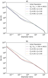 |
Fig. A.2 Same as A.1 using fke parameters: fke0 = 0.1, γ = 0.5, and β = 0. |
| In the text | |
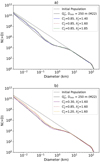 |
Fig. A.3 Same as A.1 using fke parameters: fke0 = 0.085, γ = 0.5, and β = 0.015. |
| In the text | |
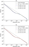 |
Fig. A.4 Same as A.1 using fke parameters: fke0 = 0.085, γ = 0.8, and β = 0.015 |
| In the text | |
|
Fig. B.1 Evolved SFDs for case 2 (unconventional scaling law with Dmin = 20 m) with parameters indicated in the legend. fke parameters: fke0 = 0.35, γ = 0.7, and β = 0. The black solid line is the reference case of M22. |
| In the text | |
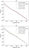 |
Fig. B.2 Same as B.1 using fke parameters: fke0 = 0.1, γ = 0.5, and β = 0. |
| In the text | |
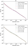 |
Fig. B.3 Same as B.1 using fke parameters: fke0 = 0.090, γ = 0.5, and β = 0.010. |
| In the text | |
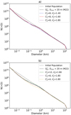 |
Fig. B.4 Same as B.1 using fke parameters: fke0 = 0.090, γ = 0.8, and β = 0.010. |
| In the text | |
Current usage metrics show cumulative count of Article Views (full-text article views including HTML views, PDF and ePub downloads, according to the available data) and Abstracts Views on Vision4Press platform.
Data correspond to usage on the plateform after 2015. The current usage metrics is available 48-96 hours after online publication and is updated daily on week days.
Initial download of the metrics may take a while.