| Issue |
A&A
Volume 701, September 2025
|
|
|---|---|---|
| Article Number | A71 | |
| Number of page(s) | 22 | |
| Section | Stellar structure and evolution | |
| DOI | https://doi.org/10.1051/0004-6361/202554539 | |
| Published online | 04 September 2025 | |
Validating and improving two-fluid simulations of the magnetic field evolution in neutron star cores
1
Departamento de Física, Facultad de Ciencias Básicas, Universidad Metropolitana de Ciencias de la Educación, Av. José Pedro Alessandri 774, Ñuñoa, Santiago, Chile
2
Departamento de Física, Facultad de Ciencias, Universidad de Chile, Las Palmeras 3425, Ñuñoa, Santiago, Chile
3
Ioffe Institute, Politekhnicheskaya 26, St. Petersburg, 194021
Russia
4
Centro de Desarrollo de Investigación UMCE, Universidad Metropolitana de Ciencias de la Educación, Santiago, Chile
⋆ Corresponding author: This email address is being protected from spambots. You need JavaScript enabled to view it.
Received:
14
March
2025
Accepted:
11
July
2025
Abstract
Context. This paper addresses the evolution of an axially symmetric magnetic field in the core of a neutron star. The matter in the core is modeled as a system of two fluids, namely neutrons and charged particles, with slightly different velocity fields controlled by their mutual collisional friction. This problem was addressed in our previous work through the “fictitious friction” approach.
Aims. We study the validity of our previous work and improve on it by comparing the fictitious friction approach to alternatives, making approximations that allow it to be applied to arbitrary magnetic field strengths and using realistic equations of state.
Methods. We assumed the neutron star crust to be perfectly resistive so that its magnetic field reacts instantaneously to changes in the core, in which we neglect the effects of Cooper pairing. We explored different approaches to solve the equations to obtain the velocities and chemical potential perturbations induced by a given fixed magnetic field configuration in the core. We also present a new version of our code to perform time-evolving simulations and discuss the results obtained with it.
Results. Our calculations without fictitious friction further confirm that bulk velocity is generally much greater than ambipolar velocity, leading to faster evolution. These findings align with those with fictitious friction, validating this approach. We also find that, in the long term, the star evolves toward a barotropic “Grad-Shafranov equilibrium,” where the magnetic force is fully balanced by charged particle fluid forces. Qualitatively, the evolution and the final equilibrium are independent of the magnetic field strength B and the equation of state considered. The timescale to reach this equilibrium is proportional to B−2 and becomes shorter for equations of state with a smaller gradient of the ratio between the densities of protons and neutrons.
Key words: magnetohydrodynamics (MHD) / methods: numerical / stars: magnetic field / stars: neutron
© The Authors 2025
 Open Access article, published by EDP Sciences, under the terms of the Creative Commons Attribution License (https://creativecommons.org/licenses/by/4.0), which permits unrestricted use, distribution, and reproduction in any medium, provided the original work is properly cited.
This article is published in open access under the Subscribe to Open model. This email address is being protected from spambots. You need JavaScript enabled to view it. to support open access publication.
1. Introduction
Neutron stars (NSs) are categorized into different classes (e.g., magnetars, rotation-powered pulsars, rotating radio transients, isolated thermal emitters) based on their observable properties (Ascenzi et al. 2024a). Efforts toward a “grand unification” (Kaspi 2010) of their vast observational phenomena have suggested that the magnetic field serves as a unifying factor (Harding 2013; Viganò et al. 2013). Consequently, the evolution of their magnetic field continues to be a relevant and active area of research. (For a recent review, see Igoshev et al. 2021.)
The current picture of magnetic field evolution in the fluid cores of NSs is as follows: Minutes after their formation, the charged particles in their interior (mostly protons, p; electrons, e; and muons, μ), which feel the magnetic force, are strongly coupled to each other and to neutrons, n, by collisions, and the particles essentially behave as a single fluid. However, their joint motion, which is driven by the magnetic force, is strongly hindered by fluid forces (pressure and gravity) that arise from stable stratification (Pethick 1992; Reisenegger & Goldreich 1992; Goldreich & Reisenegger 1992).
During this stage, sound and Alfvén waves propagate and are eventually damped, allowing the star to (very quickly) settle into a state of hydromagnetic quasi-equilibrium. The nature of such equilibria has been extensively studied in the literature, yielding geometries that vary from ordered axisymmetric “twisted-torus” configurations with poloidal and toroidal components that stabilize each other (Braithwaite & Spruit 2004, 2006; Braithwaite & Nordlund 2006) to disordered non-axisymmetric equilibrium magnetic fields (Braithwaite 2008; Becerra et al. 2022a), depending on the initial radial distribution of magnetic energy in the star (Braithwaite 2008) and the main energy dissipation mechanism invoked, namely, viscosity versus magnetic diffusivity (Becerra et al. 2022a).
While the star cools, a crust is formed; thus, the magnetic evolution continues in two different regions, a solid crust and a fluid core, with the transition between them occurring at approximately half of the nuclear saturation density. As discussed by Goldreich & Reisenegger (1992), the two long-term mechanisms that promote the evolution of the field in the crust are Ohmic diffusion (a dissipative effect due to electron-ion collisions) and Hall drift (non-dissipative advection of the magnetic field by the electrical current). The evolution of the magnetic field in this region, its effect on thermal evolution, and its potential impact on observations have been extensively studied in the literature (see, for instance, Hollerbach & Rüdiger 2002; Pons & Geppert 2007; Pons et al. 2009; Viganò et al. 2012; Gourgouliatos & Cumming 2014b; Viganò et al. 2013; Gourgouliatos & Cumming 2014a; Marchant et al. 2014; Lander & Gourgouliatos 2019; Viganò et al. 2021). Recent efforts have even involved full three-dimensional simulations (Wood & Hollerbach 2015; Dehman et al. 2023; Ascenzi et al. 2024b).
The core, on the other hand, follows a different picture. Young NSs have high temperatures, which in principle allow the core matter to overcome stable stratification while still moving as a single fluid strongly coupled by collisions. At such temperatures, the chemical imbalances due to the magnetic force are continuously reduced by weak interaction processes (Urca reactions). This erodes the initial quasi-equilibrium state, allowing the magnetic field and particles to move through a continuous sequence of quasi-equilibrium states as the chemical imbalances are reduced (Reisenegger et al. 2005; Reisenegger 2009; Ofengeim & Gusakov 2018). However, this so-called strong-coupling regime is short-lived. The star passively cools down due to Urca reactions that are faster than reheating from the feedback caused by the magnetic evolution (even for magnetar-strength fields), quickly rendering Urca reactions inefficient at restoring chemical equilibrium. Moreover, the timescale of magnetic field evolution increases very quickly as the temperature decreases (tB ∝ T−6); thus, the magnetic field is found to evolve very little at this stage (Moraga et al. 2024). As noted by Moraga et al. (2024), the latter implies that the kind of barotropic equilibrium configurations often used in the literature as initial configurations for proto-NSs (e.g., Thompson & Duncan 1996; Lander et al. 2021), which are solutions of the “Grad-Shafranov” (GS) equation (see Sect. 7.1 for details), cannot be reached in this early stage of evolution. However, as shown by Castillo et al. (2017, 2020), GS equilibrium configurations are expected to appear at later times in the so-called weak-coupling regime, which we discuss next.
As the star cools further, the collisional coupling between charged particles and neutrons is reduced, allowing for a motion of charged particles relative to neutrons in a dissipative process called ambipolar diffusion (Pethick 1992; Goldreich & Reisenegger 1992). The velocity of this relative motion is proportional to the imbalance between the magnetic force and the charged particle fluid forces it induces, and it is also inversely proportional to the collision rate between charged particles and neutrons. Such motion erodes the initial hydromagnetic quasi-equilibrium, promoting the evolution of the magnetic field and fluid forces as they continually readjust and move through a continuum of successive quasi-equilibria. In Castillo et al. (2020), we report two-fluid numerical simulations of ambipolar diffusion considering a core of normal (non-Cooper-paired) npe matter in axial symmetry. We showed that as ambipolar diffusion acts, the fluid forces due to neutrons and charged particles adjust, with the former going to zero and the latter eventually fully balancing the magnetic force. Thus, an equilibrium is reached that can only be very slowly eroded by the combination of Hall drift and Ohmic dissipation. Since charged particles are fully decoupled from neutrons, this corresponds to a single-fluid barotropic equilibrium configuration, which is a solution of the GS equation.
Ambipolar diffusion is arguably the main effect promoting the magnetic field evolution in the core (in that region, it is certainly more effective than Hall drift and Ohmic decay, as conductivity is much higher). Consequently, it has been proposed as a plausible alternative mechanism explaining the weak magnetic fields of millisecond pulsars (Cruces et al. 2019). It is also sometimes invoked to explain the activity of magnetars, as it strongly depends on the magnetic field strength (Thompson & Duncan 1995, 1996; Mereghetti 2008; Beloborodov & Li 2016; Tsuruta et al. 2023), although recent evidence suggests that it is difficult for it to account for the high thermal luminosity of some of these stars, unless their internal magnetic field is extremely strong (Moraga et al. 2025). Thus, its impact on the long-term evolution of the field is a matter of interest.
The method to self-consistently solve the relevant equations for npe matter (see Sect. 2) was introduced by Gusakov et al. (2017) and later refined by Ofengeim & Gusakov (2018). The latter authors presented a detailed scheme to semi-analytically solve the relevant system of equations for a given initial magnetic field configuration and demonstrated that, in general, the bulk motion of the particle fluids can be much larger than the relative velocity between species. This finding was confirmed by the numerical simulations of the magnetic field evolution presented in Castillo et al. (2020). Taking this into account makes the evolution significantly faster than previously estimated (e.g., Goldreich & Reisenegger 1992; Thompson & Duncan 1995; Beloborodov & Li 2016; Castillo et al. 2017; Passamonti et al. 2017).
The semi-analytical scheme proposed by Gusakov et al. (2017) and Ofengeim & Gusakov (2018), while useful to calculate the velocities and chemical potential perturbations induced by an analytically given magnetic field, has limited applicability in long-term numerical simulations, as the latter involve iterating over magnetic field data stored in tables, and these data are not given as explicit analytical expressions. The authors mention that using magnetic field configurations in the form of tables in their scheme produces unreliable results; this limitation is attributed to the high number of spatial derivatives involved in the calculation (see Sect. 2), which yield numerical errors that accumulate if iterated over time (private communication).
Alternatively, in Castillo et al. (2020), we followed a different approach. Instead of directly solving the relevant equations, we introduced a fictitious friction (FF) force acting on the neutrons. The FF approach can be regarded as a numerical trick that greatly simplifies the numerical calculation of the relevant velocities and yields a very good approximation of the solution of the relevant equations (see a detailed discussion in Sect. 4). This approach allowed us to report the first two-fluid axially symmetric numerical simulations of ambipolar diffusion, correctly capturing the bulk motion of neutrons and charged particles, which cannot be done with the one-fluid approximation usually found in the literature (e.g., Goldreich & Reisenegger 1992; Castillo et al. 2017; Igoshev et al. 2023). While definitely a step forward, that work has some features that may not be entirely convincing to some readers:
-
The approach used involved two timescales that are very different for realistic magnetic fields. To capture both in the simulations, we had to consider unrealistically high values of the magnetic field (≳1017G).
-
The FF approach is conceptually not trivial, and at first glance, it is not evident that it yields the correct velocity fields.
-
The toy model equation of state (EoS) used (see Sect. 5) correctly captured the qualitative impact of stable stratification on the long-term magnetic evolution. However, the question of whether considering more realistic models would significantly affect the reported results remains.
In this paper, we compare different methods to solving the relevant equations, including the FF approach and semi-analytical approaches based on the explicit scheme of Gusakov et al. (2017) and Ofengeim & Gusakov (2018) as well as a pseudo-spectral method. Moreover, we present the results of an updated version of the code used in Castillo et al. (2020) that addresses the issues in items 1 and 3 of the above list, and we present arguments to convince the reader about the correctness and applicability of the FF approach (thus addressing item 2 in the same list).
This paper is organized as follows. In Sect. 2, we discuss the physical model and construct the equations to be solved in axial symmetry. In Sect. 3 and Sect. 4, we describe different approaches to obtaining the relevant velocities and chemical potential perturbations. In Sect. 5 and Sect. 6, we present the different stellar and magnetic field models used in this work. In Sect. 7, we describe the relevant equations for the magnetic field evolution, discuss the relevant timescales, and outline the mechanisms that promote the dissipation of the magnetic field. Our results are presented in Sect. 8, where we compare the different approaches to obtain the neutron velocity and use the FF approach to perform long-term time-evolving simulations. We check if the simulations are in agreement with the expected timescales and final equilibrium configurations. Finally, in Sect. 9, our results are summarized and our conclusions are outlined.
2. Physical model
Following the discussion of Castillo et al. (2020), we model the NS core as a fluid composed of normal (not superfluid or superconducting) neutrons, protons, and electrons, in axial symmetry. In the absence of a magnetic field, these are in a spherically symmetric hydrostatic and chemical equilibrium, having number densities, ni(r), and chemical potentials, μi(r) (i = n, p, e), respectively. Note that charge neutrality implies nc ≡ np = ne, and chemical equilibrium implies μ ≡ μn = μp + μe.
For strong enough magnetic fields, the relative velocity of protons and electrons (related to the electric current density) is much smaller than their bulk velocity (Ofengeim & Gusakov 2018). Therefore, all charged particles are assumed to move together with velocity vc, carrying along the magnetic flux according to Faraday’s law,
 (1)
(1)
In contrast, the neutrons are allowed to move with a different velocity, vn. The main challenge in simulating this process is obtaining the velocity fields vc and vn at each time step.
In the presence of a magnetic field, B, the magnetic force causes small perturbations to the number densities of neutrons, δnn, and charged particles, δnc ≡ δnp = δne, which evolve following the continuity equations
 (2)
(2)
 (3)
(3)
Here, λ is a temperature-dependent parameter; Δμ ≡ δμc − δμn; δμc ≡ δμp + δμe; and δμn, δμp, and δμe are the chemical potential perturbations of the neutrons, protons, and electrons, respectively. The terms on the right-hand side of the equations represent the net rates per unit volume at which weak interactions convert protons and electrons into neutrons, and vice versa; assuming |Δμ|≪kBT, where kB is the Boltzmann constant and T is the absolute temperature (Goldreich & Reisenegger 1992). In what follows, we focus on the low-temperature, “weak-coupling” regime, where λ ≈ 0. Chemical potential perturbations are related to the number density perturbations, δnn, and δnc, by
 (4)
(4)
 (5)
(5)
where Kij ≡ ∂μi/∂nj (i, j = c, n). The off-diagonal element K ≡ Knc = Kcn accounts for strong interactions between protons and neutrons.
For any realistic magnetic field, the evolution timescale of such perturbations will be many orders of magnitude shorter than the magnetic evolution timescale. Therefore, in time-evolving simulations, resolving the time-evolution timescale of the density perturbations and magnetic field for a realistic magnetic field strength is computationally prohibitive. However, as shown by Gusakov et al. (2017), the time derivatives in the continuity Eqs. (2), and (3) can be safely neglected in the study of the long-term evolution, as the density perturbation of charged particles and neutrons will almost instantaneously adjust to the current configuration of the magnetic field. Thus, we reduced the continuity equations to
 (6)
(6)
 (7)
(7)
Each particle species feels fluid forces due to their weight and degeneracy pressure gradient. Namely, the fluid forces on the neutrons and charged particles are, respectively, fi = −ni∇δμi − ni(δμi/c2)∇Φ, for i = n, c; where Φ(r) is the gravitational potential. We note that the unperturbed star is in hydrostatic equilibrium, satisfying
 (8)
(8)
Thus, by the introduction of the relative chemical potential perturbations, χi = δμi/μ (i = n, c), fluid forces can be rewritten in a more compact form:
 (9)
(9)
 (10)
(10)
Charged particles also feel the Lorentz force,
 (11)
(11)
An underlying assumption is that the star very quickly reaches a state of hydromagnetic quasi-equilibrium in which all the forces acting on a fluid element are close to balance, yielding
 (12)
(12)
Consequently, in the long term, the magnetic field evolves moving through a continuum of successive hydromagnetic quasi-equilibria. In axial symmetry, the gradients, ∇χi, cannot have a toroidal component; therefore, Eq. (12) imposes a strong constraint on the magnetic field that must satisfy fB, ϕ = 0.
The relative velocity of the charged particles with respect to the neutrons is the so-called ambipolar velocity, which is obtained from the force balance on the charged particles as
 (13)
(13)
Here, γcn parametrizes the collision rate between charged particles and neutrons.
Fluid forces are written in terms of gradients of the chemical potential perturbations (see Eqs. (9) and (10)). Thus, there are additive constants in χn and χc that do not play a role in the evaluation of the velocities. If needed, these can be fixed using integral conditions corresponding to the conservation of charged particles and neutrons, i.e.,
 (14)
(14)
 (15)
(15)
where the density perturbations are obtained inverting Eqs. (4) and (5), and 𝒱core is the volume of the core.
As stated before, we restricted ourselves to axial symmetry so the magnetic field could be decomposed as
 (16)
(16)
The scalar potentials, α(r, θ), and β(r, θ), generate the poloidal and toroidal magnetic field, respectively, and  .
.
At each time step, the Lorentz force, fB, is known, but the velocity fields, vi, and the scalar fields, χi, for i = n, c must be obtained from the self-consistent solution of Eqs. (6), (7), (12), and (13). Different approaches to this challenge are discussed in Sect. 3. To perform numerical calculations using such approaches, the equations must be normalized appropriately. The units in which the different variables are measured are given in Table 1.
Normalization of the relevant variables.
Stellar parameters for the five different EoSs studied.
3. Semi-analytical approaches
3.1. Explicit approach
The set of Eqs. (6), (7), (12), and (13) can be solved for an analytically given magnetic field configuration in axial symmetry for which fB, ϕ = 0. A semi-analytical procedure to solve the set of equations was described by Gusakov et al. (2017) and more in depth by Ofengeim & Gusakov (2018). Their steps to obtain the poloidal component of the velocities and chemical potential perturbations are summarized here, adopting the notation and approximations used in the present paper.
The poloidal part of Eq. (12) implies scalar equations for the radial and polar components, respectively. For a given magnetic force, fB, these equations fix χn and χc up to a radial function for each, which can be fixed by taking the appropriate boundary conditions. However, these conditions are not trivial and must be set for vn. To proceed, we split the relative chemical imbalances into two components: χn(r, θ) = Xn(r, θ)+χn, 0(r), and χc(r, θ) = Xc(r, θ)+χc, 0(r), where  and
and  . Here, we introduced the operator
  that extracts the coefficient of the lth Legendre component of its argument,
 (17)
(17)
where f(r, θ) is a given function of r and θ, and Pl(cos θ) is a Legendre polynomial of degree l. The relation between these radial functions can be obtained by taking the radial component of Eq. (12) and projecting its 0th Legendre component
 (18)
(18)
where prime (′) denotes derivative with respect to r. Replacing the decomposition of χc and χn into Eq. (12) together with the latter equation yields
 (19)
(19)
where  , and
, and  is the radial unit vector. We note that by defining ϵ ≡ nnXn + ncXc and δ ≡ nn′Xn + nc′Xc, Eq. (19) can be rewritten as
  . The solution for ϵ and δ can be easily obtained by first integrating its polar component with respect to θ. Thus,
 (20)
(20)
 (21)
(21)
where the latter comes from the radial component and  is chosen so
  . In terms of these variables, we can reconstruct
 (22)
(22)
 (23)
(23)
which also satisfy  .
.
To fully determine χn and χc, we also needed to evaluate χn, 0 and χc, 0. We note that by integrating Eq. (6) over the volume, 𝒱(r), of any centered sphere of radius, r, we obtained
 (24)
(24)
implying  . Analogously, from Eq. (7) we obtained
  , and thus also
  . On the other hand, replacing Eq. (12) and χn = Xn + χn, 0 into Eq. (13) would yield
 (25)
(25)
Taking the radial component of the latter and projecting its 0th Legendre component implies
 (26)
(26)
This, together with Eq. (18), implies
 (27)
(27)
These conditions define χn, 0 and χc, 0 from fB, r up to additive constants that do not affect the calculation of the velocities. If needed, they can be fixed using Eqs. (14) and (15).
Finally, the velocities can be obtained as follows: vad, which is purely poloidal, can be obtained from Eqs. (25) and (26),
 (28)
(28)
whereas vn follows by writing vc = vn + vad and replacing Eq. (28) into Eq. (7), which implies
 (29)
(29)
By multiplying Eq. (6) by nc, Eq. (29) by nn, and then subtracting them, we obtained, after some algebra,
 (30)
(30)
The polar component can be obtained from Eq. (6)
 (31)
(31)
where the limits of the integral are chosen to be consistent with conditions arising from axial symmetry, i.e., vn, θ(r, 0) = vn, θ(r, π) = 0.
On the other hand, the toroidal magnetic force must remain null (∂fB, ϕ/∂t = 0), which imposes a quite complicated condition that can, in principle, be used to obtain vn, ϕ (see Ofengeim & Gusakov 2018). So far, no feasible numerical implementation to obtain vn, ϕ for an arbitrary magnetic field configuration has been proposed.
In summary, the steps to obtain the poloidal components of vn and vc for an analytically given magnetic field satisfying fB, ϕ = 0 are
-
Evaluate ϵ and δ from the magnetic force using Eqs. (20) and (21).
-
Evaluate Xn from Eq. (22).
-
Evaluate vad from Eq. (28).
-
Evaluate vn, r and vn, θ from Eqs. (30) and (31), respectively.
-
Evaluate vc, Pol = vn, Pol + vad, Pol,
where the subscript “Pol” refers to the poloidal part of a vector field,  .
.
We note that this procedure completely defines the velocity fields everywhere in the NS core, leaving no room for imposing boundary conditions at the crust-core interface. Thus, any such conditions, for example no flux of particles through the interface (vn, r(r = R) = vc, r(r = R) = 0), would require constraining the magnetic field (Ofengeim & Gusakov 2018), and it is unclear whether these constraints will be maintained as the magnetic field evolves in time.
In Sect. 8.1, we show plots of the velocities, which are computed using the procedure described above. All steps are evaluated using Wolfram Mathematica1 software, which produces involved symbolic expressions for the velocities and chemical potential perturbations in terms of the coordinates r, θ, the magnetic force, the functions nc(r),nn(r),μ(r),γcn(r), and their radial derivatives. The latter background functions are evaluated from numerical data computed from the EoS.
3.2. Pseudo-spectral approach
In addition to the semi-analytical procedure outlined in Sect. 3.1, the system of Eqs. (6), (7), (12), and (13) can be solved using a pseudo-spectral approach. An optimal implementation of such an algorithm requires rewriting some of the previous equations in a spectral-friendly manner.
Spectral codes expand scalar and vector fields using polynomial bases for the radial and angular domains within a spherical region. The angular component is typically expanded in spherical harmonics as they satisfy the regularity conditions along the axis. In axial symmetry, these reduce to the Legendre polynomials Pl(cos θ). Consequently, the chemical perturbationsread as
 (32)
(32)
where nθ represents the truncation order of the polynomial basis in the angular domain, and  ; thus Xi = ∑l ≥ 1χi, l(r)Pl(cos θ). For simplicity, we have omitted the explicit expansion of χi, l(r) in radial polynomials. The solution procedure is the following:
-
First, we computed the chemical potential perturbations. Instead of using Eqs. (22) and Eqs. (23) to obtain the {χi, l}l ≥ 1, we proceeded in the following manner. To obtain χc, we divided Eq. (12) by μnn and then took the curl
![Mathematical equation: $$ \begin{aligned} \boldsymbol{\nabla }\times \left[ \left( \frac{n_c}{n_n} \right)^{\prime } \chi _c \hat{r}\right] = - \boldsymbol{\nabla }\times \left(\dfrac{ \boldsymbol{f}_{B}}{\mu n_n}\right). \end{aligned} $$](/articles/aa/full_html/2025/09/aa54539-25/aa54539-25-eq50.gif) (33)
(33)Taking again the curl of Eq. (33) and computing only its radial component, we obtained
 (34)
(34)Here, ΔH represents the horizontal Laplacian, which in axial symmetry can be expressed as
 (35)
(35)and its eigenfunctions are the Legendre polynomials:
 (36)
(36)Thus, with the aid of equations (34)–(36), we obtained χc, l, while χn, l was determined by repeating the same procedure but dividing Eq. (12) by μnc instead. Thus, for l ≥ 1, the functions χi, l(r) read as
 (37)
(37) (38)
(38) -
Next, we obtained the velocity fields. The ambipolar velocity is the simplest to acquire, and this can be done once Xn = ∑l ≥ 1χn, l(r)Pl(cos θ) has been determined (see Eq. (28)). Since nnvn is purely solenoidal, its poloidal component can be written as
 (39)
(39)Here, Ψ(r, θ) is a scalar field. Taking the radial component of the latter and projecting its lth Legendre component yields
 (40)
(40)where
 . This, together with Eq. (30), implies
 (41)
(41)for l ≥ 1, which can be used to compute vn, θ from Eq. (39), whereas the term Ψ0 is not relevant, as it vanishes from the right-hand side of the latter equation.
These equations are solved using the pseudo-spectral code Dedalus2: a flexible framework for spectrally solving differential equations, encompassing boundary, initial, and eigenvalue problems (Burns et al. 2020). It expands in terms of Jacobi polynomials and spherical harmonics in the radial and angular domains, respectively (for more details, see, e.g., Vasil et al. 2019).
To compute the velocity field, we implemented the procedure described above. We computed χi, l (i = n, c) for l ≥ 1 by straightforward substitution in Eqs. (37) and (38). After this, obtaining vad and vn was achieved through a simple substitution in Dedalus (Eqs. (28), (39), and (41)). If needed, we could also determine χn, 0 and χc, 0. To do so, a boundary value problem is solved consisting of Eq. (18) together with conditions (26)-(27) and the integral conditions (14)-(15). In the implementation of this approach, we set the truncation order to nr = 100 and nθ = 71 radial and angular polynomials, respectively.
We note that the pseudo-spectral approach just described has the same limitations as the explicit approach. Namely, it does not provide a way to compute the toroidal component of vn and vc, which makes the approach unsuitable for time-evolving simulations, and it does not allow one to impose boundary conditions at the crust-core interface.
4. Fictitious friction approach
In Sect. 3, we showed how the set of Eqs. (6), (7), (12), and (13) can, in principle, be solved for any given magnetic field configuration. However, the numerical implementation is cumbersome, as it requires knowledge of high-order derivatives of the magnetic field (Ofengeim & Gusakov 2018). In Castillo et al. (2020), we instead introduced a FF force in Eq. (12) (see Yang et al. 1986; Roumeliotis et al. 1994; Hoyos et al. 2008, 2010; Viganò et al. 2011), defined as
 (42)
(42)
where ζ is a (small) adjustable parameter, which is a strategy that, to our knowledge, was first described by Chodura & Schlüter (1981). With this additional force, the force balance equation takes the form
 (43)
(43)
from which the neutron velocity can be determined:
 (44)
(44)
Within the framework of the FF approach, instead of solving the original system of Eqs. (6), (7), (12), and (13), it is proposed to solve a modified system consisting of equations Eqs. (6), (7), (13), and (44). This system of equations is hereafter referred to as the FF equations or the FF system, and the corresponding calculation method is called the FF approach. The main advantage of this approach is the simplicity of calculating all three components of the neutron velocity vn using Eq. (44). We note that in the limiting case ζ → ∞, we recover the one-fluid approximation, in which neutrons are modeled as a motionless background (see, e.g., Castillo et al. 2017).
However, we wanted to know how valid the FF approach is. To answer this question, we assumed that the solution of Eqs. (6), (7), (12), and (13) obtained using the rigorous method of Sect. 3.1 is known. We denote the quantities describing this solution with the superscript (0). For example,  and
and  represent the relative neutron chemical potential perturbation and neutron velocity in the quasi-stationary approximation, respectively, for a given B.
Then, we supposed that for a sufficiently small dimensionless parameter ζ (in the units specified in Table 1), the solution of the FF system can be expressed as a series expansion in ζ. For instance, for the quantities χn and vn, we can write
 (45)
(45)
 (46)
(46)
(Similar expansions are assumed to hold for other problem parameters, e.g., fc, fn.) Substituting these expansions into Eq. (44) gives
![Mathematical equation: $$ \begin{aligned} \begin{split} \gamma _{cn}n_c n_n[ \zeta \boldsymbol{v}^{(0)}_{n} +\zeta ^2\boldsymbol{v}^{(1)}_{n}+\dots ] =\,\,&[\boldsymbol{f}_{B}+\boldsymbol{f}^{(0)}_{n}+\boldsymbol{f}^{(0)}_{c}] + \\&\zeta [\boldsymbol{f}^{(1)}_{n}+\boldsymbol{f}^{(1)}_{c}] + \dots . \end{split} \end{aligned} $$](/articles/aa/full_html/2025/09/aa54539-25/aa54539-25-eq67.gif) (47)
(47)
Equating terms of the same order in ζ yields an infinite set of equations relating quantities of order k and k + 1 (k = 0, 1, …). The first two of these equations are
 (48)
(48)
![Mathematical equation: $$ \begin{aligned}&\boldsymbol{v}^{(0)}_{n} = \frac{1}{\gamma _{cn}n_c n_n}\left[\boldsymbol{f}^{(1)}_{n}+\boldsymbol{f}^{(1)}_{c} \right].&\end{aligned} $$](/articles/aa/full_html/2025/09/aa54539-25/aa54539-25-eq69.gif) (49)
(49)
The first equation is satisfied automatically, as it coincides with the force balance equation (12) of our exact problem. The second equation, in turn, provides a relationship between the neutron velocity  of the exact solution and the first-order corrections
  and
and  to the forces
  and
and  . It can be shown that the remaining Eqs. (6), (7), and (13) allow, in principle, for the complete calculation of all first-order corrections in terms of the zeroth-order quantities (computed using the rigorous approach). The higher-order terms can be found following the same strategy.
From this example, the essence of the FF approach becomes clear. Within this approach, the solution approximately corresponds to the exact solution of Eqs. (6), (7), (12), and (13) with an accuracy of 𝒪(ζ). For instance:  . Thus, for sufficiently small ζ, the FF approach should yield a solution that deviates only slightly from the exact calculation.
We have just discussed how, given the exact solution of the system Eqs. (6), (7), (12), and (13), the solution of the FF system can be derived. However, in practice, the FF approach was specifically proposed to avoid solving the exact system of Eqs. (6)–(13). Supposing we chose a sufficiently small parameter, ζ, and found the solution of the FF equations, we wanted to determine whether this solution would always be close to the exact solution of the system (6)–(13). Unfortunately, this is not the case. As discussed below, the FF system requires more boundary conditions than the original system (6)–(13). Specifically, to uniquely solve the FF equations, some boundary conditions must be imposed, for example, by specifying the r components of the velocities vn and vc at the crust-core interface. Meanwhile, in the exact system, these components are determined automatically during the solution process, as they depend on the magnetic field structure. Thus, the FF system of equations describes a broader class of solutions, which only becomes close [to an accuracy of ∼𝒪(ζ)] to the exact solution if the boundary conditions for the FF system (values of the r components of the velocities vn and vc at the boundary) are chosen to be sufficiently close to the corresponding boundary values obtained in the exact calculation. This interpretation has been verified numerically; see Sect. 8.1.2 for details. With these caveats, the FF approach can be successfully used to determine velocity fields for a given magnetic field configuration, as described below.
To solve the FF system for a given initial condition for the magnetic field, we can replace the velocities from Eqs. (13) and (44) into the continuity Eqs. (6) and (7), together with Eqs. (9) and (10). After rearranging terms, leaving only the terms explicitly dependent on the magnetic field on the right-hand side of the equations, we obtained
 (50)
(50)
![Mathematical equation: $$ \begin{aligned} \boldsymbol{\nabla }\cdot \left[n_c\mu \boldsymbol{\nabla } \chi _n + g(\zeta )n_c\mu \boldsymbol{\nabla } \chi _c \right]&= \boldsymbol{\nabla }\cdot \left[ g(\zeta ) \boldsymbol{f}_{B}\right] . \end{aligned} $$](/articles/aa/full_html/2025/09/aa54539-25/aa54539-25-eq77.gif) (51)
(51)
Here, we introduced a dimensionless radial function,
 (52)
(52)
The differential equations (50), (51), and integral conditions (14) and (15) fully define the functions χc and χn when combined with appropriate boundary conditions such as the non-penetration conditions at the crust-core interface for the velocity fields, i.e., vn, r = vad, r = 0, which translates into
 (53)
(53)
 (54)
(54)
We chose these boundary conditions because they can be easily implemented numerically. However, it should be noted that, as shown by Ofengeim & Gusakov (2018), for an arbitrary magnetic field, the exact solution to the set of Eqs. (6), (7), (12), and (13) will typically yield non-null radial components of the velocities at the boundary.
4.1. Numerical implementation using finite difference and finite volume
In order to numerically solve our equations using a finite difference and finite volume implementation, we discretize the relevant variables over a staggered polar grid composed of Nr points that can be homogeneously or inhomogeneously distributed in the radial direction and Nθ points equally spaced in the polar direction, following the rule
 (55)
(55)
 (56)
(56)
The exponent, u, is specified later. We discretized the relevant variables on this grid in the following way, where half-integer indices denote averages (e.g., ri + 1/2 ≡ (ri + ri + 1)/2):
-
The variable α was evaluated at the corner of each cell: αi, j = α(ri, θj).
-
The variable β, χn, and χc and the ϕ component of the forces and velocities were evaluated at the center of each cell: βi, j = β(ri + 1/2, θj + 1/2).
-
The radial components of vector fields, such as the magnetic field, the forces, and the velocities were evaluated at the centers of cell faces defined by a constant r = ri: Br i, j = Br(ri, θj + 1/2).
-
The polar components of vector fields, such as the magnetic field, the forces, and the velocities were evaluated at the centers of cell faces defined by a constant θ = θj: Bθ i, j = Bθ(ri + 1/2, θj).
The value of the divergence of a vector field F at the center of each cell (∇ ⋅ F)i, j = ∇⋅F|ri + 1/2, θj + 1/2 was given by
 (57)
(57)
where Fr i, j = Fr(ri, θj + 1/2), Fθ i, j = Fθ(ri + 1/2, θj); Sr i, j and Sθ i, j are the surface areas of the faces of each cell at constant r = ri and θ = θj, respectively; and 𝒱i, j is the volume of the cell. Therefore,
 (58)
(58)
Assuming boundary conditions vn, r(r = R) = vc, r(r = R) = 0, Eqs. (50) and (51) can be solved for the relative chemical perturbations, χn, and χc. Considering all grid cells, we have two sets of variables, {χn i, j}i = 1, j = 1Nr − 1, Nθ − 1 and {χc i, j}i = 1, j = 1Nr − 1, Nθ − 1, giving a total of 2(Nr − 1)(Nθ − 1) unknowns. Eqs. (50) and (51) are evaluated at the center of each grid cell. Thus, each of them provides (Nr − 1)(Nθ − 1) equations, making a total of 2(Nr − 1)(Nθ − 1). We note that these equations only involve spatial derivatives of the relative chemical perturbations. Thus, they determine χn and χc up to additive constants. Fixing these constants requires extra conditions provided by Eqs. (14) and (15). Therefore, for the system of equations to be consistent, we must replace two redundant equations from the discretization of Eqs. (50) and (51). We choose to replace the equations corresponding to the grid cell (i, j) = (1, 1).
In the evaluation of each divergence, the boundary conditions on the velocities must be taken into account. For each cell touching the symmetry axis, we impose the fluxes through the corresponding face of the cell to be null (i.e., θ = 0 or θ = π). In the cells touching the center of the star, we impose fluxes through the face defined by r = 0 to be null, and at the faces defined by r = 1 we impose vn, r = 0 and vad, r = 0, thus fluxes through those faces are null as well. In other words, radial fluxes at r = 1 of the cells touching the boundary are equal on both sides of equations (50) and (51).
Schematically, the linear system described before can be represented by a vector of unknown values of the relative chemical potential perturbations χ = {{χn i, j}i = 1, j = 1Nr − 1, Nθ − 1,{χn i, j}i = 1, j = 1Nr − 1, Nθ − 1}; a vector b containing the right-hand side of Eqs. (50), (51), (14), and (15); and a sparse matrix, Λ, generated from the coefficients extracted from the discretization of the left-hand side of the previous equation:
 (59)
(59)
We note that all the dependence on the magnetic field is in b. Thus, Λ needs to be inverted only once in a time-evolving simulation. It is also worth noting that this approach has some limitations. Setting a very small value of ζ, is not only limited by the integration time. As ζ decreases, the matrix Λ becomes progressively more singular.
In summary, this solution consists of the following steps:
-
An initial seed for the magnetic field is chosen.
-
From the magnetic field, b is computed and used to solve for the chemical potential perturbations:
 (60)
(60) -
The values of χn and χc are replaced into Eqs. (13) and (44), yielding the relevant velocities.
In the case we are also interested in following the time evolution:
-
The time derivative of the magnetic field from Eqs. (1) is computed and used to evolve the magnetic field one time step (see more details in Sect. 7).
-
This procedure is iterated, going back to step 1 but using the evolved magnetic field.
4.2. Numerical implementation with the Dedalus pseudo-spectral code
As an alternative numerical implementation of the FF approach, we solved Eqs. (50) and (51) with the normalization described in Table 1 using Dedalus. The truncation orders were set to nr = 92 for the radial polynomials and nθ = 65 for the angular polynomials. As explained in Sect. 3.2, Dedalus expands the radial and angular domains using Jacobi polynomials and spherical harmonics, respectively, leveraging their properties to solve the system in Eq. (60) efficiently.
We remark that all regularity conditions imposed by axial symmetry are naturally satisfied, as the polynomial basis used in the expansion is inherently regular at the axis and the origin. Additionally, the boundary conditions, Eqs. (53) and (54), are enforced in Dedalus using the τ-method (see, e.g., Boyd 2001).
5. Background neutron star model
We performed our analysis considering five different EoSs. One is the same toy model described in Castillo et al. (2020). There, neutrons and protons are treated as a non-relativistic Fermi gas, and electrons are treated as an extremely relativistic Fermi gas. Both neutrons and protons are considered to have the same mass m. Therefore, the chemical potentials are related to the particle densities by
 (61)
(61)
 (62)
(62)
where pFi(r) = ℏ[3π2ni(r)]1/3 (i = n, c) are the Fermi momenta of neutrons and charged particles, respectively. Thus, the density profiles can be written as
![Mathematical equation: $$ \begin{aligned} n_n(r)&=\left[\frac{2mc}{\hbar (3\pi ^2)^{1/3}}n_c(r)^{1/3} + n_c(r)^{2/3}\right]^{3/2},\end{aligned} $$](/articles/aa/full_html/2025/09/aa54539-25/aa54539-25-eq89.gif) (63)
(63)
 (64)
(64)
where sinc(x) = sin(x)/x. Equation (63) comes from the chemical equilibrium condition, μn(r) = μc(r), and Eq. (64) is an analytic approximation to the radial profile obtained by numerically integrating the (non-relativistic) stellar structure equations.
The other EoSs used are HHJ (Heiselberg & Hjorth-Jensen 1999), BSk24, BSk25, and BSk26 (Goriely et al. 2013), which have been adapted for npe matter. For all realistic models, the central density is adjusted so that the mass of the star is 1.4M⊙. The basic parameters of the stellar models are summarized in Table 2. Unlike the toy model, these realistic EoSs consider strong interactions by means of a coefficient K ≠ 0 (see Sect. 2). A comparison between nn, nc, and nc/nn as functions of r for the different models can be seen in Figs. 1(a) and (b). The collision coefficient between charged particles and neutrons, γcn, for the different models is computed from Jpn(r, T) = nc(r)nn(r)γcn(r, T) given by Yakovlev & Shalybkov (1991), where T is the temperature.
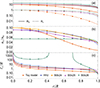 |
Fig. 1. Comparison between the five different EoSs studied. (a) nn and nc, in units of nc(r = 0); (b) the ratio nc/nn; and (c) ℓc/R, where ℓc ≡ −[dln(nc/nn)/dr]−1 (see Sect. 7.2) and R is the core radius. All these variables are functions of the normalized radial coordinate, r/R. |
6. Analytical magnetic field models
In our simulations, initial conditions are given by analytical expressions for α and β as functions of r and θ. These functions are normalized so that the rms value of the magnetic field in the core is 1:
 (65)
(65)
We focus on the following models:
Model I: Arguably, the simplest expressions for a purely poloidal magnetic configuration are of the form
 (66)
(66)
where f(r) is a polynomial on r. In particular, the following has been widely used in the literature (Akgün et al. 2013; Armaza et al. 2015; Passamonti et al. 2017; Ofengeim & Gusakov 2018; Castillo et al. 2020):
 (67)
(67)
The numerical coefficients on the polynomial come from imposing continuity of B on the surface of the core with a current-free dipole solution outside [f(r)∝1/r], continuity of the toroidal component of the current density Jϕ (although this is not a physical requirement), and the normalization of the magnetic field (in addition to a regularity condition at the axis, which does not allow for terms proportional tor0 and r1).
Model II, a model with null radial velocities at the crust-core interface: Following Ofengeim & Gusakov (2018), we can construct poloidal magnetic field configurations for which the radial components of both vn and vad vanish at the crust-core interface. First, we take α as a multipolar expansion ofthe form
 (68)
(68)
where
 (69)
(69)
Here, Cl are constants that determine the relative weights of each multipole, fl(r) = ∑ial, iri are polynomials of r, and Pl1 are the associated Legendre functions. The potentials αl are normalized so their generated magnetic field Bl ≡ ∇αl × ∇ϕ satisfies ⟨Bl⟩ = 1, implying ∑lCl2 = 1. For this model, we only considered a dipole; however, equations are written for a more general case, as they also apply to model III. The order of the polynomial(s) depends on the number of conditions to be imposed. We enforce the same three conditions as for model I, namely
 (70)
(70)
 (71)
(71)
 (72)
(72)
These are, respectively, continuity of B at the crust-core boundary considering a current-free field everywhere outside the core; continuity of Jϕ, which is null outside; and a normalization.
Additional conditions follow from setting vn, r(1, θ) = vad, r(1, θ) = 0. If we expand vad, r(1, θ), using Eq. (28), into Legendre polynomials, all Legendre components should be null, which implies  , l = 1, 2, …. Thus, the first extra condition is
 (73)
(73)
Analogously, Eq. (30) implies ![Mathematical equation: $ \hat{\mathrm{P}}_{l}\{\boldsymbol{\nabla}\cdot[(\mu/\gamma_{cn})\boldsymbol{\nabla} X_n] |_{r = 1}\} = 0 $](/articles/aa/full_html/2025/09/aa54539-25/aa54539-25-eq101.gif) , l = 1, 2, …, which, together with Eq. (73), yields the second extra condition
, l = 1, 2, …, which, together with Eq. (73), yields the second extra condition
![Mathematical equation: $$ \begin{aligned} \int _0^\pi \left[\frac{\partial ^2X_n}{\partial r^2}-\frac{l(l+1)}{r^2}X_n\right]_{r=1}P_l(\cos \theta )\sin \theta =0 ,\quad l=1,2,... \end{aligned} $$](/articles/aa/full_html/2025/09/aa54539-25/aa54539-25-eq102.gif) (74)
(74)
To apply these two conditions, we first need to obtain Xn in terms of the set of coefficients {al, i} in fl(r). This is done first by computing the magnetic force in terms of the al, i coefficients, then using (20), (21), and (22). The number of non-zero Legendre components in Xn, and consequently in Eqs. (73) and (74), increases nonlinearly with the number of non-zero Legendre components in B (as Xn is nonlinear in B). For a dipolar magnetic field configuration (corresponding to l = 1), the only non-zero Legendre component in Xn is l = 2, which imposes non-linear relations for the coefficients {al = 1, i} in Eqs. (73) and (74). We have a total of five conditions; thus, we used a polynomial of five coefficients of the form
 (75)
(75)
Solving for the coefficients, using the conditions previously described, yields eight solutions, four of which, evaluated with the HHJ EoS, are summarized in Table 3 and displayed in Fig. 2. The other four are the same, just with a global minus sign. We focus on “Solution 1” (hereafter model II, αII); as in the others, the magnetic flux is fully enclosed inside the core.
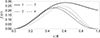 |
Fig. 2. Radial functions f1(r) for model II. The coefficients for each solution are given in Table 3. |
Model III, a non-equatorially symmetric model with null radial velocities at the crust-core interface: Using the conditions from the previous model, we can build a non-equatorially symmetric poloidal magnetic configuration with null radial velocities at the crust-core interface. For this, we consider a combination of a dipolar and quadrupolar magnetic field configuration of the form  , where
 (76)
(76)
 (77)
(77)
The number of al, i coefficients considered comes from the number of conditions needed to fix the configuration. For each of the multipoles (l = 1 and l = 2), we have to satisfy the conditions from Eqs. (70) and (72); a total of four. We note that we relaxed condition (71), as it is not strictly needed. Also, αIII yields a function, Xn(r, θ), that includes non-zero multipoles l = 1, 2, 3, and 4. Thus, Eqs. (73) and (74) yield eight equations. So, we have set enough coefficients to satisfy the 12 conditions needed for αIII. There is a very large number of solutions for this system. The coefficients for the solution we use in this work are presented in Table 4.
Model IV, a non-equatorially symmetric model with a toroidal component: We use the same non-equatorially symmetric magnetic field introduced in Castillo et al. (2020), with poloidal and toroidal components produced by the potentials
 (78)
(78)
 (79)
(79)
where
 (80)
(80)
 (81)
(81)
The quadrupolar poloidal potential, αaux, (which satisfies the same conditions as αI), and the toroidal potential, βaux, are both normalized so ⟨BPolaux⟩ = 1 and ⟨BToraux⟩ = 1, respectively3; so αIV and βIV will produce a magnetic configuration in which the toroidal magnetic field has 40% of the internal magnetic energy.
The magnetic field models I, II, III, and IV are shown in the first row of Fig. 3.
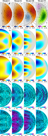 |
Fig. 3. Magnetic field configurations, relative chemical potential perturbations, and velocity fields produced by the models I, II, III, and IV. For B, lines represent the poloidal magnetic field lines labeled by the corresponding value of α. For models I–III, color represents the poloidal potential α, while in model IV, it represents the toroidal magnetic field Bϕ. For χn and χc, color represents their local value. For vn and vad, lines represent the poloidal component and color its magnitude; these are computed through the explicit semi-analytic approach described in Sect. 3.1 using the background NS model with the HHJ EoS. |
7. Time evolution
The time-evolving equations for the magnetic potentials can be obtained from Eq. (1) together with Eq. (16)
![Mathematical equation: $$ \begin{aligned} \frac{\partial \alpha }{\partial t}&=r\sin \theta \left[\left(\boldsymbol{v}_n+\boldsymbol{v}_{ad}\right)\times \boldsymbol{B}\right]\cdot \hat{\phi }, \end{aligned} $$](/articles/aa/full_html/2025/09/aa54539-25/aa54539-25-eq111.gif) (82)
(82)
![Mathematical equation: $$ \begin{aligned} \frac{\partial \beta }{\partial t}&=r^2\sin ^2\theta \boldsymbol{\nabla }\cdot \left\{ \frac{\left[\left(\boldsymbol{v}_n+\boldsymbol{v}_{ad}\right)\times \boldsymbol{B} \right]\times \hat{\phi }}{r\sin \theta } \right\} . \end{aligned} $$](/articles/aa/full_html/2025/09/aa54539-25/aa54539-25-eq112.gif) (83)
(83)
The evolution in the core and crust of the star are coupled. For simplicity, in this work we assume that the crust acts as a vacuum or perfect resistor (∇ × B = 0). Therefore, the magnetic field outside of the core can be written as B = ∇φ, where  and bl are coefficients. The magnetic field in the crust and outside of the star is entirely determined by the radial component of the magnetic field at the crust-core interface, where continuity implies
  (see Marchant et al. 2011). Of course, in practice, we are only considering a finite number of external multipoles, NExp, satisfying the criterion NExp ≥ Nθ/4. It should be noted that the assumption of a current-free crust is properly justified only if currents therein dissipate much faster than in the core. The latter, however, is very uncertain (Jones 2001; Cumming et al. 2004), and simulations coupling the evolution of the core and crust may be more appropriate (see discussion in Sect. 9, numeral 5).
In our time-evolving simulations, the numerical computation of the time derivative of the toroidal potential β is performed conservatively using a finite-volume scheme, and the time derivative of the poloidal potential α is calculated using finite differences. The decomposition of the magnetic field in terms of α and β ensures that the condition ∇ ⋅ B = 0 is maintained at all times with machine precision. The time evolution is computed using the midpoint method (a second-order Runge–Kutta method), which allows the system to be evolved with second-order accuracy in time. For more details on the numerical code, please refer to Castillo et al. (2017).
7.1. Hydromagnetic quasi-equilibrium
As discussed in Sect. 1, after a few Alfvén times, the magnetic field will evolve toward a hydromagnetic quasi-equilibrium state in which, under axial symmetry, the toroidal magnetic force must be null, since the fluid forces, fi = −niμ∇χi (i = n, c), which are purely poloidal, cannot balance it. This imposes a strong condition on the magnetic field; Eq. (16) implies fB, ϕ ∝ |∇α × ∇β| = 0; which can only be achieved if there is a relation between the magnetic potentials (e.g., β = β(α)). Since in our model there is no toroidal field outside of the core, the latter implies that the toroidal field must be confined to the regions in which the poloidal magnetic field lines close inside of the core, forming a “twisted torus” configuration (Chandrasekhar & Prendergast 1956; Braithwaite & Spruit 2004). It also implies that the magnetic force takes the form
 (84)
(84)
where
 (85)
(85)
is the so-called GS operator.
As time passes, this quasi-equilibrium is slowly eroded as the magnetic field lines, which are frozen into the charged particle fluid, keep moving relative to the neutron fluid with velocity vad. Eventually, a final barotropic equilibrium state is reached on a timescale ∼tB (see Sect. 7.2), in which the magnetic force is mainly balanced by the pressure gradient and gravitational force of the charged particle fluid, while neutrons stay in diffusive equilibrium,
 (86)
(86)
 (87)
(87)
The latter formula indeed means diffusive equilibrium, since it is equivalent to the condition ∇δμn + (δμn/c2)∇Φ = 0 (see Eq. (8) and the definition of the function χn).
Eqs. (84) and (86) imply that, in this kind of equilibrium, not only β, but also χc, must be a function of α, and these variables must satisfy the so-called GS equation
 (88)
(88)
Solutions to this equation are called “GS equilibria” (Grad & Rubin 1958; Shafranov 1966) and have been widely studied in the literature (e.g., Armaza et al. 2015 and references therein). We note that in this equilibrium χn must be uniform, but χc is non-uniform. Together with Eq. (4), this implies that, unlike what one might have expected, δnn cannot be uniform.
7.2. Time-scale estimates
From Eq. (1), we can estimate the timescale for magnetic evolution in the core of the star as
 (89)
(89)
where ℓB is the length scale over which the magnetic field varies. The usual assumptions found in the literature (Goldreich & Reisenegger 1992; Thompson & Duncan 1996; Castillo et al. 2017; Passamonti et al. 2017) are that the neutron velocity can be neglected and that the magnitude of the poloidal component of the ambipolar velocity can be estimated from Eq. (13) as vad, Pol ∼ fB/(γcnncnn) (vad, ϕ = 0 in the quasi-stationary state). From Eq. (11), we see that the magnitude of the magnetic force can be estimated as fB ∼ B2/(4πℓB). Under these assumptions, we obtain the usual estimate for magnetic evolution under ambipolar diffusion as tB ∼ tad, where
 (90)
(90)
for BSk24. This derivation, however, has a few shortcomings. First, from Eqs. (12) and (13), we see that a better estimate of the magnitude of the poloidal component of the ambipolar velocity is vad ∼ fn/(γcnncnn); however, as demonstrated by Moraga et al. (2024), an arbitrary magnetic field can induce fluid forces larger than the Lorentz force, i.e., fc ∼ fn ∼ (ℓc/ℓB)fB, where we introduced a length scale
![Mathematical equation: $$ \begin{aligned} \ell _c\equiv -\left[\frac{d}{dr}\ln (n_{c}/n_{n})\right]^{-1}, \end{aligned} $$](/articles/aa/full_html/2025/09/aa54539-25/aa54539-25-eq122.gif) (91)
(91)
which is a measure of the stable stratification due to the composition gradient in the NS core [more strongly stratified for smaller ℓc, see Fig. 1(c)]. Thus,
 (92)
(92)
More importantly, the implicit assumption of fixed neutrons is not justified. As shown in Ofengeim & Gusakov (2018) and numerically checked by Castillo et al. (2020), the neutron velocity can be much larger than the ambipolar diffusion velocity. Its magnitude can be estimated from Eqs. (9) and (30) as
 (93)
(93)
Typically, ℓc/ℓB ≫ 1 (see Sect. 8.1); therefore, from Eqs. (92) and (93), we obtain a more accurate estimate of the long-term evolution timescale of the magnetic field under ambipolar diffusion
 (94)
(94)
In the case of the FF approach, the FF force sets a shorter timescale in which the star relaxes to a state of hydromagnetic quasi-equilibrium. The velocity of the motion that causes such relaxation can be obtained from Eq. (43), which yields fB ∼ ζnnvn. Thus, the configuration of the magnetic field and particles adjusts on a timescale
 (95)
(95)
which should be identified with an Alfvén-like time and must be much shorter than the dynamical time tB of our interest for our simulations to accurately represent the long-term evolution. For this purpose, we use ζ/(γncnc) = 10−2 − 10−5 in our simulations, which satisfies this condition, but is of course much too large for a realistic Alfvén time. Since, under axial symmetry, there is no toroidal gradient of the chemical potentials to balance the toroidal magnetic force, toroidal motions will rearrange the magnetic field on a timescale tζB so the toroidal component of the force is null in the quasi-stationary state.
7.3. Magnetic energy dissipation
The loss of total magnetic energy (UB) due to ambipolar diffusion can be computed by taking the derivative of the magnetic energy and then using Eq. (1):
 (96)
(96)
where 𝒱∞ stands for all space and UB, Ext is the magnetic energy outside of the core. Integrating this expression by parts and using Eq. (11), we obtained
 (97)
(97)
which is the net power transfer between the fluids and the magnetic field. We note that the boundary term from the integration by parts (i.e., minus the Poynting flux integrated over the surface of the core) cancels with  .
.
In the case of the FF approach, the latter can be further disassembled using Eqs. (13) and (44)
 (98)
(98)
Here, we identify the energy loss due to binary collisions between charged particles and neutrons as
 (99)
(99)
and the energy loss due to the FF on the neutrons as
 (100)
(100)
The rate at which energy goes into (or comes from) the charged particles can be identified as
 (101)
(101)
This expression can be rearranged by replacing Eq. (10) and integrating by parts. Then, using Eq. (7) yields
 (102)
(102)
In the last equation, we have used Eq. (8). Thus,  could be interpreted as the mechanical work per unit time done by gravity on the charged particle fluid. Analogously, the work per unit time done by gravity on the neutrons can be identified as
 (103)
(103)
Here,  and
and  can be positive or negative. We note, however, that these terms are a direct consequence of the adopted Newtonian approximation (in particular, the way we account for redshifts) and they do not appear in the fully relativistic treatment (Gusakov et al. 2017; Moraga et al. 2025). Combining the equations above, the net rate of change of the total magnetic energy can be written as
 (104)
(104)
8. Results
8.1. Comparison between the different approaches
In this section, we compare the different methods described earlier by evaluating the neutron and ambipolar velocities. The different methods are compared to the semi-analytical velocities obtained for the magnetic field models studied in this work.
In Fig. 3, we show the relative chemical potential perturbations, χn and χc, and the velocity fields for each magnetic field model, evaluated with the explicit semi-analytical approach described in Sect. 3.1 using numerical data from the HHJ EoS. We note, however, that model IV is not in quasistationary equilibrium since, for this model, fB, ϕ is non-zero. Thus, strictly speaking, the procedure outlined in Sect. 3.1 does not apply. Aside from this caveat, we see that the neutron velocity is much larger than the ambipolar velocity for all magnetic field models studied and that this difference becomes larger as the magnetic field has a more complex structure, which is consistent with Eq. (93). This can be seen more clearly in Table 5, where the non-purely dipolar and non-equatorially symmetric models III and IV yield the largest ratios ⟨vn⟩/⟨vad⟩.
Root mean square velocities.
8.1.1. Solutions for the pseudo-spectral approach
As described in Sect. 3.2, the system of equations from Sect. 2 can be rewritten for a direct solution with a pseudo-spectral code (using Eqs. (28), (37), (38), (39), and (41)). The solution is implemented with Dedalus.
Figures 4 and 5 show radial profiles at two angles for the chemical potential perturbations and for the neutron and ambipolar velocities using magnetic field models I and II. For the pseudo-spectral approach, analytical fitting formulae for the background quantities (nn, nc, γcn, and μ; hereafter, HHJ-fit) were used (see Table 6), since using numerical data from the HHJ EoS yields incorrect results for the velocities at the crust-core interface. The slight difference between the HHJ-fit model and HHJ is shown in Fig. 6. In Figs. 4 and 5 we see there is very good agreement between the output of Dedalus and the semi-analytical solution evaluated using the explicit approach in most of the star. However, there are minor discrepancies close to the crust-core interface. This is consistent with the fact that nc, while overall quite similar in the HHJ-fit and HHJ models, differs up to ∼0.2% close to the crust-core interface (see Fig. 6).
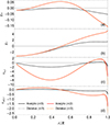 |
Fig. 4. Comparison of the pseudo-spectral approach (dashed line) and the semi-analytical solution obtained using the explicit approach (continuous line) for magnetic field model I. The solution from the pseudo-spectral approach uses a polynomial fit for the relevant background radial profiles. From top to bottom: (a) χn, (b) χc, (c) vn, r, and (d) vad, r. All quantities are in code units, plotted as functions of r for θ = π/3 and θ = π/2. |
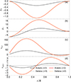 |
Fig. 5. Comparison of the output of the pseudo-spectral approach (dashed line) and the semi-analytical solution obtained using the explicit approach (continuous line) for magnetic field model II. The solution from the pseudo-spectral approach uses a polynomial fit for the relevant background radial profiles. From top to bottom: (a) χn, (b) χc, (c) vn, r, and (d) vad, r. All quantities are in code units, plotted as functions of r for θ = π/3 and θ = π/2. |
Analytical fit of the radial profiles for the HHJ EoS.
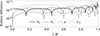 |
Fig. 6. Relative difference between the analytical fit of the radial profiles obtained for the HHJ EoS (see Table 6) and the data extracted from tables. That is, |xfit(r)/x(r)−1|, for x = nn, nc, μ, and γcn. |
8.1.2. Solutions for the FF approach
As demonstrated in Sect. 4, the velocities obtained in the FF approach will differ from the real ones, with their difference increasing with ζ. From the expression used in this approach for vn (Eq. (44)), it is not evident for what value of ζ the obtained velocities (and other relevant variables) will resemble those obtained by the explicit approach with reasonable accuracy. It is also not obvious whether this value would be large enough so we can numerically invert the matrix Λ, which, as mentioned in Sect. 4.1, becomes singular for ζ = 0. Therefore, a numerical test for different values of ζ becomes necessary.
In Fig. 7, we show a comparison between four very different values of ζ and the semi-analytical result obtained using the explicit approach, which corresponds to ζ = 0 (hereafter, we refer to ζ in the dimensionless units of Table 1). The computation is done using magnetic field model II, as this is specifically built so that vn, r = vad, r = 0 at the crust-core interface, which in the FF approach is taken as a boundary condition. It can be observed that even for values as high as ζ = 10−2, the velocities and relative chemical potential perturbations are qualitatively similar to their semi-analytical counterpart in most of the volume, but they differ in magnitude. For ζ ≤ 10−3, the different variables also show similar qualitative behavior in the whole volume, but the difference in their magnitude decreases. For instance, for ζ = 10−3, the maximum neutron velocity is ∼47% smaller than the semi-analytical value, suggesting that this value of ζ may still be too large for an accurate evaluation, for ζ = 10−4 the maximum velocity is ∼10% smaller, while for ζ = 10−5, it is just ∼1.2% smaller. In practice, as discussed in Sect. 8.2.1, for time-evolution simulations, we are using values of ζ in the range 10−4–10−3, as smaller values yield a much longer integration time.
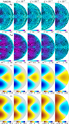 |
Fig. 7. Comparison between the explicit semi-analytical evaluation of the velocities and relative chemical potential perturbations (corresponding to ζ = 0) and the numerical calculation of the same quantities using the FF approach with different values of ζ. For vn and vad, lines represent the direction of their poloidal component and color its magnitude. This comparison is made for magnetic field model II, using the HHJ EoS. The computation is done over an equally spaced grid (u = 1 in equation (55)) of resolution Nr = 60, Nθ = 91, using an analytical expression for fB to minimize numerical errors. |
The same behavior can also be observed in Fig. 8, where we plot vn, r as a function of r for θ = π/2 for different magnetic field models and for different values of ζ, finding convergence for small ζ for all models. However, for model I, the radial velocity near the crust-core interface obtained with the FF approach differs from the one obtained using the explicit approach because the latter is not null at the crust-core interface, whereas null radial velocities are enforced as boundary conditions in the FF approach. We note, however, that the velocities are substantially different only in a thin layer of thickness ∼0.05 R. We also note that for model III the curve using ζ = 10−5 has a sudden change of sign close to r = 0, which is not observed for the other models, whose curves go smoothly to zero. This suggests that such a value of ζ may be too small, as it yields an almost-singular Λ matrix (see Eq. (59)).
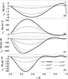 |
Fig. 8. Radial component of the neutron velocity, vn, r, for θ = π/2 as a function of r for magnetic field models I, II, III, and IV, all with the HHJ EoS. The evaluation is done with the explicit approach for ζ = 0 (no FF) and numerically using the FF approach with different values of ζ > 0. |
The equations for the FF approach can also be solved within the pseudo-spectral code Dedalus. Figures 9 and 10 compare the neutron velocity field profiles obtained through the explicit approach and the artificial friction approach, where the latter was implemented using both a finite difference method and Dedalus. The figures show magnetic field models I and II at a given angle and with the value of ζ = 10−3, using the HHJ EoS. Unlike the pseudo-spectral approach, no explicit analytical fit for the relevant background radial profile is used. The results show a very good agreement between the pseudo-spectral and the finite difference implementation of the FF approach. However, for time-evolving simulations, we restrict to the finite difference implementation, as our code was developed exactly for this purpose and has already been extensively tested.
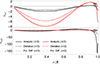 |
Fig. 9. (a) Radial and (b) polar components of the neutron velocity for θ = π/3 and θ = π/2 as functions of r for the magnetic field model I using the HHJ EoS. The evaluation is done semi-analytically (corresponding to ζ = 0; continuous line) and numerically, using the FF approach with Dedalus (dashed line) and our finite difference code (dotted line), both using ζ = 10−3. |
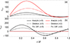 |
Fig. 10. (a) Radial and (b) polar components of the neutron velocity for θ = π/3 and θ = π/2 as functions of r for the magnetic field model II using the HHJ EoS. The evaluation is done semi-analytically (corresponding to ζ = 0; continuous line) and numerically, using the FF approach with Dedalus (dashed line) and our finite difference code (dotted line), both using ζ = 10−3. |
8.2. Hydro-magnetic evolution
In this work, we have explored different methods of obtaining the neutron and ambipolar velocities for a given magnetic field configuration, with the intention of finding a reliable method to evolve the magnetic field in time. Sadly, while we can solve the equations from Sect. 2 for analytically given magnetic field configurations using the semi-analytical approaches of Sect. 3, we have not been successful in our efforts to iterate such procedures in time to evolve the magnetic field. The reason for this seems to be related to two factors: First, the evaluation of the neutron velocity involves a large number of spatial derivatives of the magnetic field (five derivatives for vn, θ; see Sect. 3.1), which require high resolution to be solved properly. For a fixed magnetic field configuration, these can be computed to a reasonable accuracy, but in time-evolving simulations, numerical errors in their calculation accumulate. Second, for an arbitrary magnetic field, we do not have the freedom to fix boundary conditions for the velocities, whose values at the crust-core interface are completely determined by the magnetic field. Furthermore, even if the initial seed for the magnetic field is chosen to satisfy a given condition (for instance, null radial velocities), it is unclear if this magnetic field will evolve in time in such a way that the boundary conditions continue to be satisfied.
On the other hand, the FF approach offers a reliable way of evolving the magnetic field in time. Also, in the present version of the code, we have resolved some of the main caveats in the work of Castillo et al. (2020). Namely, in that version, time derivatives in the continuity Eqs. (2) and (3) were not neglected and were used to evolve the density perturbations δnn and δnc in time, which requires resolving an extremely short timescale tζp ∼ χ0 tζB ∼ 10−10(B/1013G)2 tζB, which is the analog of the propagation time of sound waves (p-modes) when inertial effects are taken into account. Thus, performing simulations in which we could numerically resolve both timescales, with the available computational resources, required artificially increasing the magnetic field strength up to unrealistic values B ≳ 1017G, so tζp and tζB could get closer. In the current version, however, time derivatives in the continuity equations are neglected, in practice replacing the need to follow the evolution of density perturbations in favor of directly solving for the chemical potential perturbations from the linear system of Eqs. (60). Therefore, the shortest timescale to be resolved in the new scheme is tζB, and the two relevant timescales, tζB and tad, scale ∝B−2, allowing us to perform simulations for one field strength and scale them to any other, as done by Moraga et al. (2024) for the magneto-thermal evolution in the high-temperature strong-coupling regime. Thus, in this subsection, we restrict ourselves to time-evolving simulations using the FF approach.
8.2.1. Convergence tests
The value of ζ used not only determines how close we are to the real velocities. In a time-evolving simulation, it also fixes the ratio between the dynamical timescales tad and tζB. For a star of B ∼ 1013 G we have an Alfvén time of tA ∼ 10 s. Since we have identified tζB with an Alfvén-like timescale, a realistic value of ζ that satisfies tA ∼ tζB would be ζ = tζB/tad ∼ 10−16 (in dimensionless units), making it impossible to resolve both timescales in a simulation. Therefore, in our simulations, we use much larger values of ζ so that both dynamical timescales are close enough to be resolved.
To determine the most appropriate range for ζ, we have performed simulations for different values, using magnetic field model II as the initial condition. These simulations were done over a non-homogeneous grid of resolution Nr = 60, Nθ = 91, setting u = 2/3 in Eq. (55). This is done so the grid cells become larger close to the center, yielding a less restrictive Courant–Friedrichs–Lewy condition (Courant et al. 1928), at the expense of losing numerical accuracy close to the center of the star. To facilitate comparison with the results of Castillo et al. (2020), hereafter we computed tad and tζB (Eqs. (90) and (95)) using B = ⟨B(t = 0)⟩, ℓB = R/4, and stellar parameters (nn, nc, γcn) evaluated at the center of the star (see Table 2). The results are in Fig. 11. It can be seen in the figure that the simulations show very similar behavior. Also, as the value of ζ gets smaller, simulations appear to converge to the same curve, particularly for ζ ≲ 10−3, which suggests that this value of ζ is good enough for our purposes.
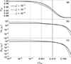 |
Fig. 11. Time evolution for magnetic field model II with background NS provided by the EOS HHJ using different values of ζ. (a) Evolution of the total magnetic energy, normalized by its initial value. (b), (c) Evolution of the rms values of the neutron velocity and ambipolar velocity, respectively. Vertical lines mark the value of tζB/tad for each simulation. |
In Sect. 8.1.2, we show how, for a fixed magnetic field, the FF approach yields velocity fields close to the semi-analytical ones only when ζ ≲ 10−5, which seems to contradict our previous statement. However, there is a key difference. In our tests with a fixed magnetic field, the only mechanism to diminish the FF force compared to the real physical forces is to take a smaller value of ζ. In time-evolving simulations, however, the magnetic field will adjust on a timescale tζB to a configuration in which the FF force progressively decreases, thereby yielding velocities that more closely approximate the real velocities. To show this more clearly, we focus on the simulation with ζ = 10−4. Snapshots of the evolution can be seen in Fig. 12. In Fig. 13(a), we observe that the FF force is always weak and becomes progressively weaker compared to the other forces, except for fn, which also decreases over time due to ambipolar diffusion. Figure 13(b) shows very good agreement between the left and right-hand sides of Eq. (104), where the left-hand side is computed explicitly as the numerical time derivative of the magnetic energy.
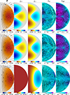 |
Fig. 12. Evolution of magnetic field model II using ζ = 10−4. We used a grid of Nr = 60 radial steps and Nθ = 91 polar steps inside the core, NExp = 40 external multipoles, u = 2/3, and the HHJ EoS. From left to right: Configuration of the magnetic field, where lines represent the poloidal magnetic field (labeled by the magnitude of α) and colors the poloidal potential α; χn and χc, both in units of χ0 = B02/4πn0μ0; neutron velocity, vn, and ambipolar diffusion velocity, vad, where arrows represent the direction and colors the magnitude normalized to R/t0. Rows correspond to different times: t = 0, t = tζB = 10−4 tad, and t = 0.1 tad. |
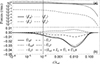 |
Fig. 13. For the simulation of Fig. 12. (a) Time evolution of the rms force densities ⟨fB⟩, ⟨fn⟩, ⟨fc⟩, and ⟨fζ⟩, all normalized by ⟨fB(t = 0)⟩. (b) Energy conservation. All terms are in units of the total initial magnetic energy. The vertical line marks tζB/tad. |
For completeness, we also include a convergence test for Nr, Nθ, and NExp. Figure 14(a) shows a fast convergence in Nr and Nθ, indicating that the grid resolution (Nr × Nθ = 60 × 91) used for the simulations in this paper is large enough. Figure 14(b) shows no significant gain by increasing the multipolar resolution when NExp > 10; this suggests that the values used in this paper (NExp = 40 for all simulations except the one displayed in Fig. 19) are large enough.
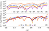 |
Fig. 14. Differences in α(r, π/2) at t = 0.1 tad for model II using different resolutions: (a) Using a fixed number of NExp = 40 external multipoles and five different grid resolutions Nr × Nθ. To aid visualization, α*, which is α at the highest resolution used (75 × 113), was subtracted. (b) Using a fixed grid resolution of 60 × 91 and five different resolutions for the number of multipoles NExp. To aid visualization, α80, which is α at the highest resolution used (NExp = 80), was subtracted. For all simulations, ζ = 10−3 and u = 2/3. |
The results described in this section apply not only to equatorially symmetric magnetic field configurations. Figure 15 shows the evolution of the magnetic energy and rms velocities for different values of ζ using the magnetic field model IV, which is more complex, as it is not equatorially symmetric and has a poloidal and a toroidal component. Here, we again see that for ζ ≲ 10−3, UB and the rms velocities appear to converge to the same curve at times larger than the value of tζB for each simulation. This is particularly evident for the toroidal part of the magnetic field, whose magnetic energy is displayed in panel (b). The rapid decay of the toroidal magnetic energy at early times, on a timescale tζB, corresponds to a rearrangement of the magnetic field in which the toroidal component of the magnetic force vanishes (see Sect. 7.1).
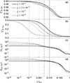 |
Fig. 15. Plots for magnetic field model IV using different values of ζ: (a), (b) Evolution of the poloidal and toroidal magnetic energy, respectively, normalized by the initial value of the magnetic energy of the star. (c), (d) Evolution of the rms poloidal neutron and ambipolar velocity. Vertical lines correspond to the value of tζB/tad in each simulation. |
8.2.2. Long-term evolution
In Sect. 8.2.1, we have shown that the FF approach is a reliable method for performing simulations for the long-term evolution of the magnetic field under ambipolar diffusion. Here, we further describe the output of such simulations.
We focus on the evolution of magnetic field model II in a star with background density profiles obtained from the HHJ EoS. This simulation was also analyzed in the previous section, and snapshots of the evolution are given in Fig. 12. In this figure, we see that the magnetic field evolution occurs in two stages: First, there is a small adjustment to the magnetic field configuration and density perturbations on a timescale tζB, in which the FF force, which is initially small due to the chosen value of ζ, becomes even smaller [see Fig. 13(a)], indicating that the magnetic field approaches a state of quasi-equilibrium in which Eq. (12) is satisfied.
This quasi-equilibrium state is slowly eroded by ambipolar diffusion. As the charged particles move relative to the neutrons, the magnetic field and particles adjust, moving through a continuum of successive hydromagnetic quasi-equilibria and eventually reaching a final equilibrium state in which vn = vad = 0. This occurs on a timescale tB, which for the simulation shown in Fig. 12 is roughly at tB ≃ 0.1tad, as can be appreciated in Fig. 13(a). We observe in Fig. 11(b) and (c) that in this final state, the fluid velocities indeed become very small, thus halting the evolution of the field.
As discussed in Sect. 7.1, this kind of axially symmetric equilibrium is called GS equilibrium, in which α is a solution of the GS Eq. (88), χc = χc(α), and χn is uniform. This can be observed in the last row of Fig. 12 and in Fig. 16 (at t = 0.1tad), suggesting that effectively the magnetic field has evolved toward a GS equilibrium.
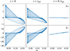 |
Fig. 16. For the simulation of Fig. 12: scatter plot of χn and χc versus α for t = 0, t = tζB, and t = 0.1tad. |
The conclusions obtained from the time evolution of magnetic field model II remain true for more complex configurations such as model IV, which has poloidal and toroidal components that are not equatorially symmetric. Snapshots of the time evolution for this model can be observed in Fig. 17, while the evolution of the rms forces is in Fig. 18(a), and the energy conservation is shown in Fig. 18(b). We note that the magnetic field is initially not in a state of quasi-equilibrium, as it has a strong toroidal magnetic force. As expected, this toroidal force becomes progressively weaker, evolving on a timescale tζB. In Fig. 17 at t = tζB, we see how quasi-equilibrium is not yet reached as β is not a function of α. This condition is more clearly satisfied at t = 5tζB, where ⟨fB, Tor⟩/⟨fB, Pol⟩≈6 × 10⁻³. Here, we also see that the toroidal magnetic field is confined to regions of closed poloidal field lines, forming “twisted tori,” which is a consequence of the condition β = β(α). At this point, χn and χc are of the same order. However, as the system evolves due to ambipolar diffusion, χn becomes progressively smaller and more uniform [see ⟨fn⟩ in Fig. 18(a)]. As expected, after the GS equilibrium is reached, χc is a function of α, and the velocities are much smaller than their initial values, indicating that the system has reached its final equilibrium.
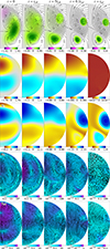 |
Fig. 17. Evolution of magnetic field model IV, using ζ = 10−3. We used a grid of Nr = 60 radial steps and Nθ = 91 polar steps inside the core and NExp = 40 external multipoles, and the HHJ EoS. From top to bottom: Configuration of the magnetic field, where lines represent the poloidal magnetic field (labeled by the magnitude of α) and colors the toroidal potential β; χn and χc, both in units of χ0 = B02/4πn0μ0; poloidal component of the neutron velocity, vn, and ambipolar diffusion velocity, vad, where arrows represent the direction and colors the magnitude normalized to R/t0. Columns correspond to different times: t = 0, tζB, 5 tζB, 0.1 tad, and tad. |
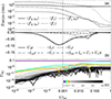 |
Fig. 18. For the simulation of Fig. 17: (a) Time evolution of the rms force densities ⟨fB, Pol⟩, ⟨fB, Tor⟩, ⟨fn⟩, ⟨fc⟩, and ⟨fζ, Pol⟩, all normalized by ⟨fB, Pol(t = 0)⟩. (b) Energy conservation. The different terms are in units of the total initial magnetic energy. (c) External magnetic energy stored in multipole l, UB, l, normalized by the total initial magnetic energy, where l = 1, …, NExp. The vertical line corresponds to tζB/tad. |
Figure 18(b) shows energy conservation for this simulation. There is overall good agreement between the curves of  , and
, and  , aside from a very small mismatch around t ∼ 0.05tad, which we attribute to numerical viscosity. Compared to the simulation of Fig. 12, here we see a larger contribution of Lζ. This is because of two factors. First, in this simulation, the magnetic field is initially not in a quasi-equilibrium state. Thus, there is a noticeable initial rearrangement of the field and the fluids on a timescale tζB. During the initial rearrangement, energy is dissipated due to physical processes that involve the propagation and damping of sound and Alfvén waves, which in our model are mimicked by the FF. The rate at which this energy is dissipated is accounted for in Lζ. In this early stage, we have vn ∼ fB/(ζnn), thus Lζ ∼ ζnnvn2R3 ∝ 1/ζ. Therefore, the energy dissipated during the unwinding of the magnetic field lines is ∼LζtζB, which does not depend on ζ (as long as it is small enough). Second, after the star reaches hydromagnetic quasi-equilibrium, vn converges to the real velocity, which does not depend on ζ, and therefore Lζ ∝ ζ, which is larger in this simulation (ζ = 10−3 for the simulation of Fig. 17 and 10−4 for the simulation of Fig. 12). For completeness, Fig. 18(c) shows energy stored in each multipole of the magnetic field outside the core. We note that multipoles l ≥ 4 do not make a relevant contribution to the energy throughout the time evolution. We also note that even for more complex initial conditions such as model IV, only a small number of external multipoles is needed to properly resolve the external field evolution. Thus, the number of multipoles used in our simulations, NExp ≥ 27, is large enough.
The results presented in this section are consistent with those reported in Castillo et al. (2020). The time evolution for all simulations presented here qualitatively follows the same stages, and in all cases, the final state corresponds to a GS equilibrium. For completeness, Fig. 19 shows a comparison between the final equilibrium state for model IV, computed by the current version of the code, which, as mentioned before, can be rescaled to any realistic value of the magnetic field strength; and the results presented in Castillo et al. (2020) for the same magnetic field model, in a simulation performed for an unrealistically high magnetic field strength of B0 = 1.8 × 10¹⁷G. We see that the final equilibrium configuration reported in Castillo et al. (2020) is correctly reproduced, and it is found not to be significantly affected by the, now realistic, magnetic field strength used.
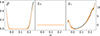 |
Fig. 19. Scatter plot of β, χn, and χc versus α for the final equilibrium configuration (at t = tad) of magnetic field model IV for two simulations, using the toy model EoS. Blue dots correspond to the results presented in Castillo et al. (2020), which are computed using B0 = 1.8 × 10¹⁷G (i.e., χ0 = 1.67 × 10⁻³); orange dots correspond a simulation performed with the current version of the code, using ζ = 3 × 10⁻³, Nr = 60 radial steps, Nθ = 91 polar steps inside the core, NExp = 27 external multipoles, and u = 1/2 (the same parameters as in Castillo et al. 2020). All quantities are normalized as described in Table 1. |
8.2.3. Dependence on the equation of state
In Castillo et al. (2020), we performed our simulations using the toy model EoS, described in Sec. 5. While it is a simple analytical model, it helped us correctly analyze the impact of the stable stratification of NS matter on the magnetic field evolution. However, the question remains if using more realistic density profiles could significantly impact the evolution of the field. In particular, in real NSs, strong interactions may play a significant role, which could not be observed in the previous simulations using the toy model.
Here, as detailed in Sect. 5, we use the EoSs HHJ, BSk24, BSk25, and BSk26, all of which consider the effect of strong interactions on the chemical potentials by means of a coefficient K ≠ 0. Results for simulations using the purely poloidal magnetic field model III with ζ = 10−3 are shown in Fig. 20. Here, we see how, for all EoSs considered, the magnetic field decays and eventually reaches an equilibrium state [see panel (a)], but the time at which this occurs for each is not the same. The toy model reaches equilibrium on a timescale ∼0.1 tad, simulations using HHJ, BSk24, and BSk25 reach equilibrium in ∼0.05 tad, while for BSk26 equilibrium is reached around 0.01 tad. These results are consistent with Eq. (94), which states that the timescale for magnetic field evolution under ambipolar diffusion is shorter than tad by a factor (ℓB/ℓc)2. In this comparison, only ℓc varies between EoSs, as seen in Fig. 1(c), while ℓB remains unchanged. We note that the toy model yields the smallest value of ℓc for all r and thus the largest estimate for tB among the stellar models studied. Regarding HHJ, BSk24, and BSk25, they yield similar values of ℓc, while in comparison, BSk26 yields the largest value and thus the shortest estimate for tB. This is further supported by Fig. 20(b)-(d), where we see the rms velocities and their ratio ⟨vad⟩/⟨vn⟩ as functions of time. We note that this ratio remains ∼0.2 for most of the evolution when using the radial density profiles from the toy model. In contrast, for BSk26, this ratio is considerably lower (∼0.02), consistent with Eq. (93).
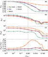 |
Fig. 20. Time evolution for the initial purely poloidal magnetic field model III with five different EoSs using ζ = 10−3, a grid of Nr = 60 radial steps, Nθ = 91 polar steps inside the core, NExp = 40 external multipoles, and u = 2/3. The panels show the following variables: (a) Magnetic energy in the NS core, normalized by its initial value. (b) and (c) rms neutron and ambipolar velocity, ⟨vn⟩ and ⟨vad⟩, respectively. (d) The ratio ⟨vad⟩/⟨vn⟩. For each model, the timescales tζB and tad, and the velocities are evaluated considering the stellar parameters of Table 2. The vertical line marks the dimensionless value of ζ = tζB/tad, which is fixed to be the same for all EoSs. |
Results for magnetic field model IV, also using ζ = 10−3, can be seen in Fig. 21. Panels (a) and (b) show the evolution of the poloidal and toroidal magnetic energy, respectively; we again see how, for the BSk26 star, the poloidal magnetic energy decays faster than for the other stellar models. On the other hand, the toroidal magnetic field decays faster for the toy model than for all the other EoSs, all of which decay on a similar timescale. The dissipation of the toroidal energy occurs mainly due to the unwinding of the toroidal magnetic field in the regions with poloidal field lines closing outside the core (see Sect. 7.1), a process with a typical timescale tζB. This timescale is proportional to nn (see Eq. (95)), which decreases toward the surface of the star (we note that in the plots, the timescales are evaluated at the center of the star). Thus, the unwinding of the field lines close to the surface is expected to be faster. Figure 1(a) shows that close to the crust-core interface, nn is smaller for the toy model EoS than for the more realistic EoSs, explaining the faster decay of the toroidal field for that case. Also, the magnetic field in that region is stronger in model IV than in model III, making the difference in nn have a larger impact on the evolution of the magnetic energy. Thus, it is not that surprising that the toroidal magnetic energy decays faster for the simulation using the (unrealistic) toy model. Consequently, the toroidal component of the velocities is expected to be larger for the toy model; panels (c) and (d) of Fig. 21 show that, for the toy model EoS, the rms values of the neutron and ambipolar velocity are larger than for the other EoSs, as these velocity averages are dominated by the toroidal component of the velocities. We note that the curves for ⟨vad⟩/⟨vn⟩ follow a similar trend to the simulation in Fig. 20. That is, for the toy model EoS, which has the largest ratio ℓB/ℓc, we have the highest ⟨vad⟩/⟨vn⟩ ratio. For the more realistic EoSs – HHJ, BSk24, and BSk25 – the neutron velocity is considerably larger than the ambipolar velocity, consistent with a ratio ℓB/ℓc ≃ 0.07. In turn, in the simulation using BSk26, the ratio ℓB/ℓc is much smaller, consistent with Fig. 1(c).
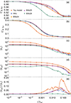 |
Fig. 21. Same as Fig. 20 but for model IV. The variables shown in each panel are: (a), (b) Poloidal and toroidal magnetic energy in the NS core, respectively, normalized by the initial value of the total magnetic energy of the NS core. (c), (d) Root mean square neutron and ambipolar velocity, ⟨vn⟩ and ⟨vad⟩, respectively. (e) Ratio of ⟨vad⟩/⟨vn⟩. |
9. Discussion and conclusions
The evolution of the magnetic field of an NS is probably responsible for much of its observed phenomenology. Initially, the magnetic field likely permeates the entire interior of the star. Therefore, understanding its evolution requires studying the key mechanisms driving it, both in the crust and the core. While crustal processes have been extensively studied and are largely understood, the same cannot yet be said for processes in the core.
Assuming an NS core composed only of “normal” (non-Cooper-paired) neutrons, protons, and electrons, its magnetic field is carried by a joint motion of the charged particles (protons and electrons), which is similar to that of the neutrons but crucially not identical because of the different density profiles entering their continuity equations (6) and (7). Their slight difference (ambipolar diffusion) causes a collisional friction that controls the timescale of this evolution, which is much longer than any of the dynamical timescales of the NS core, such as the periods of sound, gravity, or Alfvén waves. Thus, this two-fluid system can be considered to be always near a state of hydromagnetic equilibrium, where the inertial terms in the equations of motion can be ignored. In this regime, the velocity fields are determined from the force-balance and continuity equations for the two fluids (neutrons and charged particles).
Under the assumption of axial symmetry, the velocity fields of neutrons and charged particles were studied semi-analytically by Gusakov et al. (2017) and Ofengeim & Gusakov (2018) and calculated numerically by Castillo et al. (2020), who also used them to simulate the long-term evolution of the magnetic field in the NS core. For this purpose, a small FF force on the neutrons was introduced, which simplified the calculation of the velocity fields, allowing them to be calculated at every time step in order to follow the long-term evolution of the magnetic field. We found that this evolution ultimately always leads to an equilibrium state in which the magnetic force is balanced by the internal forces of the charged-particle fluid, thus satisfying the barotropic GS equation, while the neutrons reach a diffusive equilibrium that remains unaffected by the magnetic field.
In the present paper, we have addressed a few potential weaknesses of the simulations of Castillo et al. (2020), as stated in Sect. 1:
-
The approach used involved two timescales that are very different for realistic magnetic fields. To capture both in the simulations, it was only possible to consider unrealistically high values of the magnetic field (≳1017G).
-
The FF approach used in Castillo et al. (2020) is conceptually non-trivial. At first glance, it is not evident that it correctly reproduces the velocities needed to perform long-term time-evolving simulations.
-
The toy model EoS we used (see Sect. 5) correctly captured the qualitative impact of stable stratification on the long-term magnetic evolution. However, the question of whether considering more realistic EoSs would significantly affect the results remains.
In order to address item 1 of the above list, we followed Moraga et al. (2024) in neglecting the time derivatives of the density perturbations in the continuity equations, thus eliminating a short timescale that was not interesting for the magnetic field evolution. This leaves only two fundamental timescales (tζB and tad) that are both ∝B−2, and this allows the simulation results to be scaled to any relevant magnetic field strength.
Item 2 in the same list was addressed analytically by showing that the exact chemical potential perturbations and velocity fields for a given magnetic field configuration correspond to the zeroth-order term in an expansion of the equations with FF in powers of the coefficient ζ. It was further addressed by comparing numerical calculations of the same quantities for both the exact equations (following an explicit and a pseudo-spectral approach) and those with FF using different values of ζ and finding good agreement for a small ζ. These calculations were done using our grid-based code developed in-house and compared against its equivalent implementation using the Dedalus code. Moreover, by following the evolution for different values of ζ, we also find convergence for sufficiently small values. However, we note that the FF approach allows one to impose boundary conditions at the crust-core interface so that no particle flows through the latter, whereas in the equations without FF, this is only possible for specific magnetic field configurations satisfying constraints that may not continue to be satisfied throughout the evolution.
Based on the semi-analytical velocities obtained using the explicit and pseudo-spectral approaches, we provide further evidence supporting the fact that the ambipolar velocity is typically much smaller than the neutron velocity (particularly for EoS BSk26, ⟨vad⟩/⟨vn⟩∼0.02) and that their ratio decreases for more complex magnetic fields. Accounting for neutron motion leads to a much faster dissipation of the magnetic field by ambipolar diffusion. Our timescale estimate for this process (for BSk24) is
 (105)
(105)
which roughly agrees with magnetar timescales.
Finally, item 3 of the above list was addressed by evolving the magnetic field for different state-of-the-art EoSs, as well as the toy model EoS, where we find qualitative agreement. The main quantitative difference is a faster evolution of the poloidal magnetic field for EoSs with smaller composition gradients.
In summary, this paper validates our previous work by supporting the correctness of the FF approximation and improves on it by neglecting the time derivatives of the density perturbations and including realistic EoSs. There are, however, several ingredients not considered in this paper that should be considered in future work:
-
Temperature evolution: As the temperature evolves in parallel with the magnetic field, it gradually changes the values of microphysical coefficients such as collisional couplings, thus changing the timescale for the evolution of the magnetic field. On the other hand, magnetic dissipation mechanisms affect the thermal evolution of the neutron star. This magneto-thermal evolution in the NS core is being considered in Moraga et al. (2024) and Moraga et al. (2025).
-
Magnetohydrodynamic instabilities: It is unclear if the GS equilibrium remains stable (or if stability is ever even reached) if full three-dimensional motions are allowed, as there are many non-axially symmetric instabilities that may destabilize such equilibria (Tayler 1973; Markey & Tayler 1973; Wright 1973; Flowers & Ruderman 1977). Moreover, in this state, the Lorentz force is balanced only by the charged-particle fluid consisting of protons and electrons, which behaves as a barotropic fluid. Numerical simulations suggest that there are no stable equilibria in barotropic stars (Braithwaite 2009; Akgün et al. 2013; Lander & Jones 2012; Mitchell et al. 2015; Becerra et al. 2022a,b) and that even axially symmetric instabilities can be triggered, destabilizing the field (Becerra et al. 2022b). These instabilities might still be triggered in the two-fluid system at hand, although slowed by the collisional friction between the two fluids.
-
Muons: Adding additional species such as muons makes the charged-particle component non-barotropic, leading to less constrained equilibria that are not GS. Thus, even if magnetic fields in barotropic stars are always unstable, muons might stabilize them by stably stratifying the charged particle fluid.
-
Superfluidity and superconductivity: At typical core temperatures, NS matter is expected to be both superfluid and superconducting. Numerical simulations have begun incorporating these effects in simplified models (see, e.g., Bransgrove et al. 2018, 2025); we note, however, that some of the microphysical input used in these studies has been criticized (Gusakov 2019). Nucleon superfluidity and superconductivity not only influence the kinetic coefficients governing magnetic field dissipation but also lead to the formation of quantized neutron vortices and magnetic flux tubes. These effects can significantly impact the magnetic field evolution described here, altering both the characteristic timescales and the structure of the final equilibrium configuration – if such a configuration exists (see Gusakov et al. 2020 for a discussion).
-
The crust: Here, for simplicity, we have assumed the crust to be a perfect resistor, so its magnetic field reacts instantaneously to changes in the core. This is not physically justified, making it necessary to follow the evolution both in the crust and in the core in order to be astrophysically realistic. However, so far, there have been few attempts to do this. One work that has done so is Viganò et al. (2021), in which the magneto-thermal evolution of the crust is coupled with the evolution of the core, including ambipolar diffusion, although neutron motion is neglected. The recent work of Skiathas & Gourgouliatos (2024) takes a similar approach. However, in both cases, the treatment of the core is still simplified. Thus, more realistic simulations would be desirable. Whether the magnetic field evolution is faster in the core or crust depends mainly on the strength of the field and the compositional impurity of the crust and whether the matter in the core has undergone a superfluid or superconducting transition (Cumming et al. 2004; Pons & Geppert 2007; Gourgouliatos et al. 2016; Akgün et al. 2018). If the evolution is slower in the crust, it could stabilize the magnetic field in the core, leading to different kinds of equilibria.
Data availability
The data underlying this article will be shared on reasonable request to the corresponding author.
The prefactor of αaux given in Castillo et al. (2020) is not correct.
Acknowledgments
This work was supported by the CAS-ANID fund N°CAS220008 (F.C.), FONDECYT Projects 11230837 (F.C.), 1201582 (A.R.), and 1240697 (J.A.V.), and ANID doctoral fellowship 21210909 (N.A.M.). M.E.G. acknowledges support from the Ministry of Science and Higher Education of the Russian Federation under the state assignment FFUG-2024-0002 of the Ioffe Institute. N.A.M. and F.C. thank the University of Leeds for their hospitality.
References
- Akgün, T., Reisenegger, A., Mastrano, A., & Marchant, P. 2013, MNRAS, 433, 2445 [Google Scholar]
- Akgün, T., Cerdá-Durán, P., Miralles, J. A., & Pons, J. A. 2018, MNRAS, 481, 5331 [CrossRef] [Google Scholar]
- Armaza, C., Reisenegger, A., & Valdivia, J. A. 2015, ApJ, 802, 121 [Google Scholar]
- Ascenzi, S., Graber, V., & Rea, N. 2024a, Astropart. Phys., 158, 102935 [NASA ADS] [CrossRef] [Google Scholar]
- Ascenzi, S., Viganò, D., Dehman, C., et al. 2024b, MNRAS, 533, 201 [NASA ADS] [CrossRef] [Google Scholar]
- Becerra, L., Reisenegger, A., Valdivia, J. A., & Gusakov, M. E. 2022a, MNRAS, 511, 732 [NASA ADS] [CrossRef] [Google Scholar]
- Becerra, L., Reisenegger, A., Valdivia, J. A., & Gusakov, M. E. 2022b, MNRAS, 517, 560 [NASA ADS] [CrossRef] [Google Scholar]
- Beloborodov, A. M., & Li, X. 2016, ApJ, 833, 261 [NASA ADS] [CrossRef] [Google Scholar]
- Boyd, J. P. 2001, Chebyshev and Fourier Spectral Methods, 2nd edn. (Mineola, NY: Dover Publications), Dover Books on Mathematics [Google Scholar]
- Braithwaite, J. 2008, MNRAS, 386, 1947 [Google Scholar]
- Braithwaite, J. 2009, MNRAS, 397, 763 [NASA ADS] [CrossRef] [Google Scholar]
- Braithwaite, J., & Nordlund, Å. 2006, A&A, 450, 1077 [NASA ADS] [CrossRef] [EDP Sciences] [Google Scholar]
- Braithwaite, J., & Spruit, H. C. 2004, Nature, 431, 819 [Google Scholar]
- Braithwaite, J., & Spruit, H. C. 2006, A&A, 450, 1097 [NASA ADS] [CrossRef] [EDP Sciences] [Google Scholar]
- Bransgrove, A., Levin, Y., & Beloborodov, A. 2018, MNRAS, 473, 2771 [CrossRef] [Google Scholar]
- Bransgrove, A., Levin, Y., & Beloborodov, A. M. 2025, ApJ, 979, 144 [Google Scholar]
- Burns, K. J., Vasil, G. M., Oishi, J. S., Lecoanet, D., & Brown, B. P. 2020, Phys. Rev. Res., 2, 023068 [NASA ADS] [CrossRef] [Google Scholar]
- Castillo, F., Reisenegger, A., & Valdivia, J. A. 2017, MNRAS, 471, 507 [Google Scholar]
- Castillo, F., Reisenegger, A., & Valdivia, J. A. 2020, MNRAS, 498, 3000 [Google Scholar]
- Chandrasekhar, S., & Prendergast, K. H. 1956, Proc. Nat. Acad. Sci., 42, 5 [Google Scholar]
- Chodura, R., & Schlüter, A. 1981, J. Comput. Phys., 41, 68 [NASA ADS] [CrossRef] [Google Scholar]
- Courant, R., Friedrichs, K., & Lewy, H. 1928, Math. Ann., 100, 32 [Google Scholar]
- Cruces, M., Reisenegger, A., & Tauris, T. M. 2019, MNRAS, 490, 2013 [NASA ADS] [CrossRef] [Google Scholar]
- Cumming, A., Arras, P., & Zweibel, E. 2004, ApJ, 609, 999 [NASA ADS] [CrossRef] [Google Scholar]
- Dehman, C., Viganò, D., Pons, J. A., & Rea, N. 2023, MNRAS, 518, 1222 [Google Scholar]
- Flowers, E., & Ruderman, M. A. 1977, ApJ, 215, 302 [Google Scholar]
- Goldreich, P., & Reisenegger, A. 1992, ApJ, 395, 250 [NASA ADS] [CrossRef] [Google Scholar]
- Goriely, S., Chamel, N., & Pearson, J. M. 2013, Phys. Rev. C, 88, 024308 [NASA ADS] [CrossRef] [Google Scholar]
- Gourgouliatos, K. N., & Cumming, A. 2014a, Phys. Rev. Lett., 112, 171101 [NASA ADS] [CrossRef] [Google Scholar]
- Gourgouliatos, K. N., & Cumming, A. 2014b, MNRAS, 438, 1618 [CrossRef] [Google Scholar]
- Gourgouliatos, K. N., Wood, T. S., & Hollerbach, R. 2016, Proc. Nat. Acad. Sci., 113, 3944 [Google Scholar]
- Grad, H., & Rubin, H. 1958, J. Nucl. Energy, 7, 284 [Google Scholar]
- Gusakov, M. E. 2019, MNRAS, 485, 4936 [Google Scholar]
- Gusakov, M. E., Kantor, E. M., & Ofengeim, D. D. 2017, Phys. Rev. D, 96, 103012 [Google Scholar]
- Gusakov, M. E., Kantor, E. M., & Ofengeim, D. D. 2020, MNRAS, 499, 4561 [Google Scholar]
- Harding, A. K. 2013, Front. Phys., 8, 679 [Google Scholar]
- Heiselberg, H., & Hjorth-Jensen, M. 1999, ApJ, 525, L45 [Google Scholar]
- Hollerbach, R., & Rüdiger, G. 2002, MNRAS, 337, 216 [NASA ADS] [CrossRef] [Google Scholar]
- Hoyos, J., Reisenegger, A., & Valdivia, J. A. 2008, A&A, 487, 789 [NASA ADS] [CrossRef] [EDP Sciences] [Google Scholar]
- Hoyos, J. H., Reisenegger, A., & Valdivia, J. A. 2010, MNRAS, 408, 1730 [CrossRef] [Google Scholar]
- Igoshev, A. P., Popov, S. B., & Hollerbach, R. 2021, Universe, 7, 351 [NASA ADS] [CrossRef] [Google Scholar]
- Igoshev, A. P., Hollerbach, R., & Wood, T. 2023, MNRAS, 525, 3354 [Google Scholar]
- Jones, P. B. 2001, MNRAS, 321, 167 [Google Scholar]
- Kaspi, V. M. 2010, Proc. Nat. Acad. Sci., 107, 7147 [NASA ADS] [CrossRef] [Google Scholar]
- Lander, S. K., & Gourgouliatos, K. N. 2019, MNRAS, 486, 4130 [NASA ADS] [CrossRef] [Google Scholar]
- Lander, S. K., & Jones, D. I. 2012, MNRAS, 424, 482 [Google Scholar]
- Lander, S. K., Haensel, P., Haskell, B., Zdunik, J. L., & Fortin, M. 2021, MNRAS, 503, 875 [Google Scholar]
- Marchant, P., Reisenegger, A., & Akgün, T. 2011, MNRAS, 415, 2426 [NASA ADS] [CrossRef] [Google Scholar]
- Marchant, P., Reisenegger, A., Valdivia, J. A., & Hoyos, J. H. 2014, ApJ, 796, 94 [Google Scholar]
- Markey, P., & Tayler, R. J. 1973, MNRAS, 163, 77 [CrossRef] [Google Scholar]
- Mereghetti, S. 2008, A&ARv, 15, 225 [NASA ADS] [CrossRef] [Google Scholar]
- Mitchell, J. P., Braithwaite, J., Reisenegger, A., et al. 2015, MNRAS, 447, 1213 [Google Scholar]
- Moraga, N. A., Castillo, F., Reisenegger, A., Valdivia, J. A., & Gusakov, M. E. 2024, MNRAS, 527, 9431 [Google Scholar]
- Moraga, N. A., Castillo, F., Ofengeim, D. D., et al. 2025, arXiv e-prints [arXiv:2505.18733] [Google Scholar]
- Ofengeim, D. D., & Gusakov, M. E. 2018, Phys. Rev. D, 98, 043007 [Google Scholar]
- Passamonti, A., Akgün, T., Pons, J. A., & Miralles, J. A. 2017, MNRAS, 465, 3416 [Google Scholar]
- Pethick, C. J. 1992, in Structure and Evolution of Neutron Stars, eds. D. Pines, R. Tamagaki, & S. Tsuruta, 115 [Google Scholar]
- Pons, J. A., & Geppert, U. 2007, A&A, 470, 303 [NASA ADS] [CrossRef] [EDP Sciences] [Google Scholar]
- Pons, J. A., Miralles, J. A., & Geppert, U. 2009, A&A, 496, 207 [NASA ADS] [CrossRef] [EDP Sciences] [Google Scholar]
- Reisenegger, A. 2009, A&A, 499, 557 [NASA ADS] [CrossRef] [EDP Sciences] [Google Scholar]
- Reisenegger, A., & Goldreich, P. 1992, ApJ, 395, 240 [Google Scholar]
- Reisenegger, A., Prieto, J. P., Benguria, R., Lai, D., & Araya, P. A. 2005, in Magnetic Fields in the Universe: From Laboratory and Stars to Primordial Structures, eds. E. M. de Gouveia dal Pino, G. Lugones, & A. Lazarian, AIP Conf. Ser., 784, 263 [Google Scholar]
- Roumeliotis, G., Sturrock, P. A., & Antiochos, S. K. 1994, ApJ, 423, 847 [Google Scholar]
- Shafranov, V. D. 1966, Rev. Plasma Phys., 2, 103 [NASA ADS] [Google Scholar]
- Skiathas, D., & Gourgouliatos, K. N. 2024, MNRAS, 528, 5178 [NASA ADS] [CrossRef] [Google Scholar]
- Tayler, R. J. 1973, MNRAS, 161, 365 [CrossRef] [Google Scholar]
- Thompson, C., & Duncan, R. C. 1995, MNRAS, 275, 255 [Google Scholar]
- Thompson, C., & Duncan, R. C. 1996, ApJ, 473, 322 [NASA ADS] [CrossRef] [Google Scholar]
- Tsuruta, S., Kelly, M. J., Nomoto, K., et al. 2023, ApJ, 945, 151 [Google Scholar]
- Vasil, G., Lecoanet, D., Burns, K., Oishi, J., & Brown, B. 2019, J. Comput. Phys.: X, 3, 100013 [Google Scholar]
- Viganò, D., Pons, J. A., & Miralles, J. A. 2011, A&A, 533, A125 [NASA ADS] [CrossRef] [EDP Sciences] [Google Scholar]
- Viganò, D., Pons, J. A., & Miralles, J. A. 2012, Comput. Phys. Commun., 183, 2042 [Google Scholar]
- Viganò, D., Rea, N., Pons, J. A., et al. 2013, MNRAS, 434, 123 [CrossRef] [Google Scholar]
- Viganò, D., Garcia-Garcia, A., Pons, J. A., Dehman, C., & Graber, V. 2021, Comput. Phys. Commun., 265, 108001 [CrossRef] [Google Scholar]
- Wood, T. S., & Hollerbach, R. 2015, Phys. Rev. Lett., 114, 191101 [Google Scholar]
- Wright, G. A. E. 1973, MNRAS, 162, 339 [NASA ADS] [CrossRef] [Google Scholar]
- Yakovlev, D. G., & Shalybkov, D. A. 1991, Ap&SS, 176, 191 [Google Scholar]
- Yang, W. H., Sturrock, P. A., & Antiochos, S. K. 1986, ApJ, 309, 383 [NASA ADS] [CrossRef] [Google Scholar]
All Tables
All Figures
|
Fig. 1. Comparison between the five different EoSs studied. (a) nn and nc, in units of nc(r = 0); (b) the ratio nc/nn; and (c) ℓc/R, where ℓc ≡ −[dln(nc/nn)/dr]−1 (see Sect. 7.2) and R is the core radius. All these variables are functions of the normalized radial coordinate, r/R. |
| In the text | |
|
Fig. 2. Radial functions f1(r) for model II. The coefficients for each solution are given in Table 3. |
| In the text | |
|
Fig. 3. Magnetic field configurations, relative chemical potential perturbations, and velocity fields produced by the models I, II, III, and IV. For B, lines represent the poloidal magnetic field lines labeled by the corresponding value of α. For models I–III, color represents the poloidal potential α, while in model IV, it represents the toroidal magnetic field Bϕ. For χn and χc, color represents their local value. For vn and vad, lines represent the poloidal component and color its magnitude; these are computed through the explicit semi-analytic approach described in Sect. 3.1 using the background NS model with the HHJ EoS. |
| In the text | |
|
Fig. 4. Comparison of the pseudo-spectral approach (dashed line) and the semi-analytical solution obtained using the explicit approach (continuous line) for magnetic field model I. The solution from the pseudo-spectral approach uses a polynomial fit for the relevant background radial profiles. From top to bottom: (a) χn, (b) χc, (c) vn, r, and (d) vad, r. All quantities are in code units, plotted as functions of r for θ = π/3 and θ = π/2. |
| In the text | |
|
Fig. 5. Comparison of the output of the pseudo-spectral approach (dashed line) and the semi-analytical solution obtained using the explicit approach (continuous line) for magnetic field model II. The solution from the pseudo-spectral approach uses a polynomial fit for the relevant background radial profiles. From top to bottom: (a) χn, (b) χc, (c) vn, r, and (d) vad, r. All quantities are in code units, plotted as functions of r for θ = π/3 and θ = π/2. |
| In the text | |
|
Fig. 6. Relative difference between the analytical fit of the radial profiles obtained for the HHJ EoS (see Table 6) and the data extracted from tables. That is, |xfit(r)/x(r)−1|, for x = nn, nc, μ, and γcn. |
| In the text | |
|
Fig. 7. Comparison between the explicit semi-analytical evaluation of the velocities and relative chemical potential perturbations (corresponding to ζ = 0) and the numerical calculation of the same quantities using the FF approach with different values of ζ. For vn and vad, lines represent the direction of their poloidal component and color its magnitude. This comparison is made for magnetic field model II, using the HHJ EoS. The computation is done over an equally spaced grid (u = 1 in equation (55)) of resolution Nr = 60, Nθ = 91, using an analytical expression for fB to minimize numerical errors. |
| In the text | |
|
Fig. 8. Radial component of the neutron velocity, vn, r, for θ = π/2 as a function of r for magnetic field models I, II, III, and IV, all with the HHJ EoS. The evaluation is done with the explicit approach for ζ = 0 (no FF) and numerically using the FF approach with different values of ζ > 0. |
| In the text | |
|
Fig. 9. (a) Radial and (b) polar components of the neutron velocity for θ = π/3 and θ = π/2 as functions of r for the magnetic field model I using the HHJ EoS. The evaluation is done semi-analytically (corresponding to ζ = 0; continuous line) and numerically, using the FF approach with Dedalus (dashed line) and our finite difference code (dotted line), both using ζ = 10−3. |
| In the text | |
|
Fig. 10. (a) Radial and (b) polar components of the neutron velocity for θ = π/3 and θ = π/2 as functions of r for the magnetic field model II using the HHJ EoS. The evaluation is done semi-analytically (corresponding to ζ = 0; continuous line) and numerically, using the FF approach with Dedalus (dashed line) and our finite difference code (dotted line), both using ζ = 10−3. |
| In the text | |
|
Fig. 11. Time evolution for magnetic field model II with background NS provided by the EOS HHJ using different values of ζ. (a) Evolution of the total magnetic energy, normalized by its initial value. (b), (c) Evolution of the rms values of the neutron velocity and ambipolar velocity, respectively. Vertical lines mark the value of tζB/tad for each simulation. |
| In the text | |
|
Fig. 12. Evolution of magnetic field model II using ζ = 10−4. We used a grid of Nr = 60 radial steps and Nθ = 91 polar steps inside the core, NExp = 40 external multipoles, u = 2/3, and the HHJ EoS. From left to right: Configuration of the magnetic field, where lines represent the poloidal magnetic field (labeled by the magnitude of α) and colors the poloidal potential α; χn and χc, both in units of χ0 = B02/4πn0μ0; neutron velocity, vn, and ambipolar diffusion velocity, vad, where arrows represent the direction and colors the magnitude normalized to R/t0. Rows correspond to different times: t = 0, t = tζB = 10−4 tad, and t = 0.1 tad. |
| In the text | |
|
Fig. 13. For the simulation of Fig. 12. (a) Time evolution of the rms force densities ⟨fB⟩, ⟨fn⟩, ⟨fc⟩, and ⟨fζ⟩, all normalized by ⟨fB(t = 0)⟩. (b) Energy conservation. All terms are in units of the total initial magnetic energy. The vertical line marks tζB/tad. |
| In the text | |
|
Fig. 14. Differences in α(r, π/2) at t = 0.1 tad for model II using different resolutions: (a) Using a fixed number of NExp = 40 external multipoles and five different grid resolutions Nr × Nθ. To aid visualization, α*, which is α at the highest resolution used (75 × 113), was subtracted. (b) Using a fixed grid resolution of 60 × 91 and five different resolutions for the number of multipoles NExp. To aid visualization, α80, which is α at the highest resolution used (NExp = 80), was subtracted. For all simulations, ζ = 10−3 and u = 2/3. |
| In the text | |
|
Fig. 15. Plots for magnetic field model IV using different values of ζ: (a), (b) Evolution of the poloidal and toroidal magnetic energy, respectively, normalized by the initial value of the magnetic energy of the star. (c), (d) Evolution of the rms poloidal neutron and ambipolar velocity. Vertical lines correspond to the value of tζB/tad in each simulation. |
| In the text | |
|
Fig. 16. For the simulation of Fig. 12: scatter plot of χn and χc versus α for t = 0, t = tζB, and t = 0.1tad. |
| In the text | |
|
Fig. 17. Evolution of magnetic field model IV, using ζ = 10−3. We used a grid of Nr = 60 radial steps and Nθ = 91 polar steps inside the core and NExp = 40 external multipoles, and the HHJ EoS. From top to bottom: Configuration of the magnetic field, where lines represent the poloidal magnetic field (labeled by the magnitude of α) and colors the toroidal potential β; χn and χc, both in units of χ0 = B02/4πn0μ0; poloidal component of the neutron velocity, vn, and ambipolar diffusion velocity, vad, where arrows represent the direction and colors the magnitude normalized to R/t0. Columns correspond to different times: t = 0, tζB, 5 tζB, 0.1 tad, and tad. |
| In the text | |
|
Fig. 18. For the simulation of Fig. 17: (a) Time evolution of the rms force densities ⟨fB, Pol⟩, ⟨fB, Tor⟩, ⟨fn⟩, ⟨fc⟩, and ⟨fζ, Pol⟩, all normalized by ⟨fB, Pol(t = 0)⟩. (b) Energy conservation. The different terms are in units of the total initial magnetic energy. (c) External magnetic energy stored in multipole l, UB, l, normalized by the total initial magnetic energy, where l = 1, …, NExp. The vertical line corresponds to tζB/tad. |
| In the text | |
|
Fig. 19. Scatter plot of β, χn, and χc versus α for the final equilibrium configuration (at t = tad) of magnetic field model IV for two simulations, using the toy model EoS. Blue dots correspond to the results presented in Castillo et al. (2020), which are computed using B0 = 1.8 × 10¹⁷G (i.e., χ0 = 1.67 × 10⁻³); orange dots correspond a simulation performed with the current version of the code, using ζ = 3 × 10⁻³, Nr = 60 radial steps, Nθ = 91 polar steps inside the core, NExp = 27 external multipoles, and u = 1/2 (the same parameters as in Castillo et al. 2020). All quantities are normalized as described in Table 1. |
| In the text | |
|
Fig. 20. Time evolution for the initial purely poloidal magnetic field model III with five different EoSs using ζ = 10−3, a grid of Nr = 60 radial steps, Nθ = 91 polar steps inside the core, NExp = 40 external multipoles, and u = 2/3. The panels show the following variables: (a) Magnetic energy in the NS core, normalized by its initial value. (b) and (c) rms neutron and ambipolar velocity, ⟨vn⟩ and ⟨vad⟩, respectively. (d) The ratio ⟨vad⟩/⟨vn⟩. For each model, the timescales tζB and tad, and the velocities are evaluated considering the stellar parameters of Table 2. The vertical line marks the dimensionless value of ζ = tζB/tad, which is fixed to be the same for all EoSs. |
| In the text | |
|
Fig. 21. Same as Fig. 20 but for model IV. The variables shown in each panel are: (a), (b) Poloidal and toroidal magnetic energy in the NS core, respectively, normalized by the initial value of the total magnetic energy of the NS core. (c), (d) Root mean square neutron and ambipolar velocity, ⟨vn⟩ and ⟨vad⟩, respectively. (e) Ratio of ⟨vad⟩/⟨vn⟩. |
| In the text | |
Current usage metrics show cumulative count of Article Views (full-text article views including HTML views, PDF and ePub downloads, according to the available data) and Abstracts Views on Vision4Press platform.
Data correspond to usage on the plateform after 2015. The current usage metrics is available 48-96 hours after online publication and is updated daily on week days.
Initial download of the metrics may take a while.