| Issue |
A&A
Volume 701, September 2025
|
|
|---|---|---|
| Article Number | A247 | |
| Number of page(s) | 21 | |
| Section | Planets, planetary systems, and small bodies | |
| DOI | https://doi.org/10.1051/0004-6361/202554552 | |
| Published online | 19 September 2025 | |
Machine learning spectral clustering techniques: Application to Jovian clouds from Juno/JIRAM and JWST/NIRSpec
1
Department of Physics, University of Rome “La Sapienza”,
Piazzale Aldo Moro 2,
00185
Rome,
Italy
2
INAF – Istituto di Astrofisica e Planetologia Spaziali (INAF-IAPS),
Via Fosso del Cavaliere 100,
I-00133
Rome,
Italy
3
School of Physics and Astronomy, University of Leicester,
University Rd,
Leicester
LE1 7RH,
UK
4
Facultad de Ingeniería y Ciencias, Universidad Adolfo Ibáñez,
8170121
Santiago,
Chile
5
Department of Astronomy, University of California,
Berkeley,
CA
94720,
USA
6
LIRA, Observatoire de Paris, Université PSL, CNRS, Sorbonne Université, Université Paris-Cité,
Meudon,
France
7
Space Sciences Laboratory, University of California,
Berkeley
CA
94720-7450,
USA
8
Carl Sagan Center for Research, SETI Institute,
Mountain View,
CA
94043,
USA
9
Escuela de Ingeniería de Bilbao, Universidad del País Vasco,
UPV/EHU,
Bilbao,
Spain
10
Department of Mathematics, Physics and Electrical Engineering, Northumbria University,
Newcastle upon Tyne,
UK
11
Atmospheric, Oceanic and Planetary Physics, Department of Physics, University of Oxford,
Oxford,
UK
12
Agenzia Spaziale Italiana,
Via del Politecnico, snc,
00133
Roma,
Italy
13
Max Planck Institute for Solar System Research,
Justus-von-Liebig-Weg 3,
37077
Göttingen,
Germany
14
Jet Propulsion Laboratory, California Institute of Technology,
4800 Oak Grove Dr,
Pasadena,
CA
91109,
USA
15
NASA Goddard Space Flight Center, Code 693,
Greenbelt,
MD
20771,
USA
16
Department of Climate and Space Sciences and Engineering, Univ. of Michigan,
2455 Hayward St,
Ann Arbor,
MI
48109,
USA
17
Southwest Research Institute,
6220 Culebra Rd,
San Antonio,
TX
78238,
USA
★ Corresponding author.
Received:
15
March
2025
Accepted:
24
July
2025
Abstract
We present a new method, based on a joint application of a principal component analysis (PCA) and Gaussian mixture models (GMM), to automatically find similar groups of spectra in a collection. We applied the method (condensed in the public code chopper.py) to archival Jupiter spectral data in the 2–5 µm range collected by NASA Juno/JIRAM in its first perijove passage (August 2016) and to mosaics of the great red spot (GRS) acquired by JWST/NIRSpec (July 2022). Using JIRAM data analyzed in previous work, we show that using a PCA+GMM clustering can increase the efficiency of the retrieval stage without any loss of accuracy in terms of the retrieved parameters. We show that a PCA+GMM approach is able to automatically identify spectra of known regions of interest (e.g., belts, zones, GRS) belonging to different clusters. The application of the method to the NIRSpec data leads to detection of substructures inside the GRS, which appears to be composed of an outer halo characterized by low reflectivity and an inner brighter main oval. By applying these techniques to JIRAM data, we were able to identify the same substructure. We remark that these new structures have not been seen before at visible wavelengths. In both cases, the spectra belonging to the inner oval have solar and thermal signals comparable to those belonging to the halo, but they present broadened 2.73 µm solar-reflected peaks. Performing forward simulations with the NEMESIS radiative transfer suite, we propose that the broadening may be caused by differences in the vertical extension of the main cloud layer. This finding is consistent with recent 3D fluid dynamics simulations.
Key words: methods: data analysis / techniques: miscellaneous / planets and satellites: atmospheres / planets and satellites: individual: Jupiter
© The Authors 2025
 Open Access article, published by EDP Sciences, under the terms of the Creative Commons Attribution License (https://creativecommons.org/licenses/by/4.0), which permits unrestricted use, distribution, and reproduction in any medium, provided the original work is properly cited.
This article is published in open access under the Subscribe to Open model. This email address is being protected from spambots. You need JavaScript enabled to view it. to support open access publication.
1 Introduction
With the advent of state-of-the-art technology, data volumes acquired by astronomy surveys and space missions have increased exponentially. In planetary sciences, the technological development of new propulsion systems, materials, and designs increases the number and quality of scientific instruments on board space missions. An example can be seen in the exploration of the Martian system1. In the first decade of the 21th century, three NASA missions orbit Mars: Mars Global Surveyor (Bandfield et al. 2000; Malin & Edgett 2001; Christensen et al. 2001; Malin et al. 2007), Mars Odyssey Orbiter (Christensen et al. 2004), and Mars Reconnaissance Orbiter (McEwen et al. 2007; Murchie et al. 2007; Mustard et al. 2008). The respective data volumes from each instrument processed on board and throughout the primary and extended missions are: ≃1.2 TB, >2.5 TB, and 3 PB. As another example, the Breakthrough Listen project (Enriquez et al. 2017) in its search forExtraTerrestrial Intelligence (SETI) accumulates a few tens of PB/day (but gets down-sampled) on radio telescopes.
The increasing complexity and dimension of the datasets have a huge impact on the required data analysis procedures. In the context of multiple scattering atmospheric retrievals, for example, it is fundamental to use very efficient radiative transfer solvers to reach convergence as quickly as possible to analyze the maximum number of spectra. However, radiative transfer simulations execution timescale with the number of wavelength sampling points (or channels) and the number of parameters. This can result in execution times on the orders of minutes (or seconds in the best scenario), which translates into retrieval convergence times on the order of several hours for a single spectrum (or tens of minutes in the best scenario). This makes it very difficult to use all the collected spectra, which often translates into a loss of information and leads to a sub-optimal exploitation of the dataset. Therefore, to tackle the increase in complexity and scale of the data volumes, it is mandatory to develop efficient techniques that are based on Astrostatistics, Astroinformatics, machine learning (ML), or artificial intelligence (AI) and explored in across a range of studies (Lebofsky et al. 2019; Brzycki et al. 2020; Gajjar et al. 2022; Ma et al. 2023; Baumeister et al. 2020; Nixon & Madhusudhan 2020; Ardévol Martínez et al. 2024; Hayes et al. 2020).
Jupiter’s atmosphere is an excellent example of a rich and ever-expanding dataset and there have been some previous attempts to reduce the dimensionality of the data. The work from Simon-Miller et al. (2001) is one of the first to have applied PCA to the multispectral pixels of the images acquired by HST/WFPC2. Dyudina et al. (2001) used the same methods to analyze the optical and infrared (IR) images collected by SSI and NIMS on board NASA’s Galileo mission, respectively. Wong et al. (2023) applied PCA to HST/WFC3 methane-band imaging data and found that components attributed to cloud opacity predicted the observed intensity in simultaneous five-micron IR images. Studies such as those by Ordonez-Etxeberria et al. (2016), Anguiano-Arteaga et al. (2021), and Anguiano-Arteaga et al. (2023) used PCA on images acquired by HST and Cassini, combining it with clustering techniques (e.g., k-means or nearest neighbors) to identify zones of physical interest. The main rationale behind these works is to perform PCA on the two-dimensional (2D) image arrays taken at different wavelengths to find principal components that are connected to physical properties (e.g., different cloud altitudes, composition, etc.). This is conceptually different from working directly on spectra. The clustering of high-dimensional datasets, such as spectra, is usually a complex and degenerate task but is becoming more important with modern advancements in multi-object spectroscopy (Ellis et al. 2017; Yang et al. 2022). To the best of our knowledge, the only work that applied PCA directly to Jovian spectra is that of Irwin & Dyudina (2002), who analyzed Galileo/NIMS spectral cubes. Similarly, clustering based on deep learning algorithms has been applied to Cassini/VIMS data of the 2008 storm on Saturn (Waldmann & Griffith 2019). Deep learning algorithms have also been recently used to efficiently and robustly model and characterize Jupiter’s interior structure starting from gravity, wind fields, and isotopic composition measurements (Ziv et al. 2024a,b).
In this work, we present a new approach based on machine learning techniques, that combines PCA with Gaussian mixture models (GMMs) to automatically identify groups of similar spectra automatically. For this purpose, a fully Pythonic code, chopper.py, has been developed (Biagiotti 2025)2,3. The code is completely generic, however, we applied it to Jupiter observations collected during the first perijove passage by Juno/JIRAM (August 2016) and by JWST/NIRSpec during its Early Release Science phase (July 2022). The main focus of our work is the study of clouds and haze properties, namely, altitudes, optical depth, and effective radii. A special focus is placed the great red spot (GRS), the largest and longest-lived vortex in the solar system (Sánchez-Lavega et al. 2024). We demonstrate that this method can immensely reduce the computational effort during the multiple-scattering retrieval stage by identifying subsets of self-similar spectra in advance. We also show that the technique can identify clusters of spectra that correlate with known structures from visible images, along with new ones that had gone previously undetected at optical wavelengths. We detected two substructures inside the GRS: an outer low reflectivity halo and an inner brighter main oval, which not have previously been characterized.
This paper is organized as follows. In Sect. 2 we present the observations, focusing on the reduction and data-cleaning procedures performed in order to apply the clustering analysis. In Sect. 3, we present chopper.py, its simple architecture, theoretical background, and limitations. In Sect. 4, we present the results of applying this new tool to JIRAM and NIRSpec data. Lastly, in Sect. 5, we discuss the detection of the low-reflectivity halo substructure found inside the GRS, its physical possible origin, and consequences.
2 Observations
In this work, we analyze data from two near-infrared (NIR) spectrometers: JIRAM, onboard NASA’s Juno Mission (Bolton et al. 2017b,a), and NIRSpec (Jakobsen et al. 2022), one of the pay-load instruments of the James Webb Space Telescope. JIRAM is an image-spectrometer, built and designed in Italy, thanks to a collaboration between Leonardo, ASI, and INAF-IAPS (Adriani et al. 2017, 2018; Mura et al. 2018). It is capable of splitting the collected optical beam into two channels: an imager and a spectrometer. The spectra collected by JIRAM have a spectral range between 2 and 5 µm, with 336 sampling points at a resolution of almost 9 nm.
Juno is a rotating spacecraft, and at every rotation, JIRAM can acquire 256 spectra along its spectral slit. In this work, we only used the spectral data collected by JIRAM in its first perijove passage (August 2016), hereafter PJ1, that represents a unique dataset, excellent both in spectral and spatial resolution and spatial coverage. Most of the Jovian disk has been mapped, as shown in Fig. 1a, which presents a map of the signal at 5 µm superimposed to a mosaic obtained by JunoCam (see Grassi et al. 2021 and Biagiotti et al. 2025 for details). The latitudes from − 65° to +65° have a very good spatial resolution of a few tens of km. In this work, we focus on two subsets of the PJ1 data, represented in panels b and c of Fig. 1, namely:
G+21 subset: a subset of the data presented in Grassi et al. (2021), as shown in panel b at 2.7 µm. These spectra cover a large longitude span of the southern hemisphere, including: (i) a fraction of the GRS and of the oval BA (Sanchez-Lavega et al. 2001; Wong et al. 2011); (ii) a fraction of the equatorial zone (EZ); (iii) the south equatorial belt (SEB); (iv) a large fraction of the south tropical zone (STrZ); and (v) the south temperate belt (STeB). The spectra were all selected on the basis of their having incidence (i) and emission (ε) angles between 40° and 50°. This selection criterion is the primary cause of the gaps in longitude coverage. However, retaining only spectra with similar viewing angles ensures that the variance in the dataset is driven by the physical properties of clouds instead of geometry. This is a fundamental step to take before using techniques such as PCA, which are largely dependent on the covariance matrix of the data.
GRS subset: a mosaic of spectra of the GRS and its surrounding region is shown in panel c at 2.7 µm. Since the constraint on viewing conditions imposed on the previous dataset would result in a very limited spatial coverage, we decided to select spectra that only satisfy the condition 40°<i<50°. This condition would result in emission angles between 55° and 80°.
NIRSpec is the integral field unit spectrograph of the James Webb Space Telescope (Gardner et al. 2006; Jakobsen et al. 2022). The NIRSpec/IFU instrument was used, together with NIRCam and MIRI, to acquire high-quality spatially resolved spectral maps of Jupiter and of the other planets and satellites of our Solar System (Villanueva & Milam 2023). MIRI observed the GRS region (Harkett et al. 2024), offering new insights into the thermal winds and the inhomogeneities in the temperature and compositional structures. The NIRSpec maps tend to span a 3 × 3″ field-of-view (FOV), so they had to be mosaicked in a 2 × 3 pattern to ensure wide spatial coverage (Fletcher et al. 2024). As part of the early-release science (ERS, PIs: de Pater & Fouchet) program 1373, six mosaic tiles were used to map the GRS (Melin et al. 2024) and the south polar domain on 2022-07-27 using gratings G235H and G395H. Each of the spectra collected with the G235H grating (solar mosaics) consists of 3814 spectral points that span the 1.66–3.17 µm range. With the G395H grating (thermal mosaics) a total of 3610 spectral points were obtained, spanning the 2.87–5.27 µm range. NIRSpec data were reduced and navigated using the JWST pipeline and custom Solar System processing (King et al. 2023), mitigating the effects of spikes, of saturation in reflectivity peaks near ≃2 µm, along with the strong thermal emission at 5 µm by subdividing long integrations into shorter durations (known as groups). The reduced mosaics acquired with the two gratings have been later combined. As the acquisitions are vary over time, they do not precisely point at the same region on the Jovian disk. To combine them then, we first performed a manual alignment keeping only the spaxels (pixels on the map where the spectrum was acquired) that satisfy the conditions: latG235H – latG395H < 0.2° and lonG235H – lonG395H < 0.2°. Here, latG235H and lonG235H represent the latitude and longitude of the spaxels contained in the solar mosaics, while lonG235H and lonG395H are the latitude and longitude of the spaxels contained in the thermal mosaics. The chosen threshold of 0.2° was selected because it represents one-third of the mean distance of adjacent spaxels. The results of this manual alignment are shown in Fig. A.1. The spectra of the spaxels that satisfy the condition are retained and merged. The mosaic of the GRS as observed by NIRSpec at 2.7 µm is shown in panel d of Fig. 1. NIRSpec observations were acquired at viewing angles that satisfy these conditions: 20°<i<40° and 20º<ε<40º. Figure 2 shows a comparison between a spectrum of the inner regions of the GRS as seen by JIRAM (top panel) and NIRSpec (bottom panel). NIRSpec’s spectral and spatial resolution is much better than JIRAM. The disadvantage of NIRSpec is the small coverage of the planet, the small variation of phase angle in the data and the scarcity of Jupiter data that has been obtained from JWST. Unfortunately, the JIRAM and NIRSpec in our case were not close in time (with a difference of eight years) but JIRAM represents the best set of spectra collected by a space mission orbiting Jupiter to compare to the JWST observations.
Before applying techniques that are sensitive to the data variance and covariance such as PCA, it is mandatory to perform a further cleaning step in addition to the reduction. Spikes, corrupted spectra, and missing values can all add instrumental spectral effects that will bias the result of the PCA. Therefore, we performed two different data cleaning procedures on JIRAM and NIRSpec data, discussed in the next subsections. A summary of the used data cleaning procedures can be found in Table A.1.
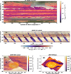 |
Fig. 1 (a) Spatial distribution of all the JIRAM PJ1 collected and non-corrupted spectra. (b) Spatial map of radiance measured at 2.73 µm for the G21 susbset of PJ1 data considered in this work. (c) Spatial map of radiance measured at 2.73 µm for the GRS susbset of PJ1 data. (d) Spatial maps of radiance measured by JWST/NIRSpec at 2.73 µm. |
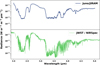 |
Fig. 2 Comparison between two spectra of the GRS captured, respectively, by Juno/JIRAM (top panel) and JWST/NIRSpec (bottom panel). It is possible to note the higher spectral resolution of NIRSpec, which must not be confused with noise. |
2.1 JIRAM data cleaning
The most significant source of instrumental-induced variance in JIRAM data is the occurrence of frequent spikes in the spectra. They are both caused by cosmic rays and energetic particles in the Jovian magnetosphere. To remove them we applied a modified version of the algorithm presented in Whitaker & Hayes (2018). The method is very efficient in correcting Raman spectra, but it can be detrimental if the spectra present reflectance peaks and absorption dips larger than the median signal. Therefore, we did not apply the Whitaker & Hayes (2018) algorithm to the whole JIRAM spectrum at once and, instead, we used it separately on three different regions of the spectrum:
the solar reflectance peaks between 2 and 2.1 µm, and 2.6 and 2.8 µm, approximately;
the 5-µm region, masking the absorption features of deuterated methane (CH3D), phosphine (PH3), ammonia (NH3), water (H2O), germane (GeH4), and arsine (AsH3);
the remaining spectral regions.
Following (Whitaker & Hayes 2018), we selected threshold value of five. With this approach, it was possible to remove the majority of the spurious spikes present in the JIRAM spectra as shown in Fig. A.2, where a representative spectrum is shown before and after the correction. After the spike correction, the G+21 subset contains 11180 spectra, each of them constituted by 336 spectral points, while the GRS subset contains 3763 spectra.
2.2 NIRSpec data cleaning
As the NIRSpec data were already reduced using the methods in King et al. (2023), we did not apply the spike correction method mentioned in the previous section. In this case, the most significant source of possible instrumental-induced variance is the occurrence of missing values in the individual spectra. These missing values can arise because of gaps between the gratings and/or residual saturation. The top panel of Fig. A.3 represents the distribution of missing values as a function of wavelength. The missing values reach a number comparable to the number of total spectra (dashed red line) in the following wavelength windows:
from 1.66 to 1.8 µm;
between 2.17 and 2.5 µm;
between 3.95 and 4.25 µm;
from 4.73 to 5.2 µm.
These windows will be referred to as “contaminated”. The second and third windows are caused by the physical gaps between the two NIRSpec detectors. The 1.8 µm window is instead caused by the very bright reflection of solar radiation by clouds. The GRS and its surroundings are well known to be one of the most cloudy regions of the Jovian disk. Lastly, the remaining window is caused by saturation induced by the planet’s internal radiation. The 4.5–5.5 µm region is generally known to be an atmospheric window, which probes deep and warm atmospheric layers whose thermal emission reaches high, saturating, radiances. The number of missing values in the 2.6–2.8 µm and 4.–4.6 µm windows is much lower than the number of total spectra. This is proof of the overall excellent work done by the reduction pipeline (King et al. 2023). These two windows are very interesting as they are related to the second brightest reflection peak and to the transition region between the solar and thermal dominated regions of the Jovian spectrum. Once the distribution of the missing values was known, we proceeded as follows:
we removed all the spectra that present a number of missing values larger than 2000;
we cut the four windows listed above that presented the highest number of counts in missing values;
we imputed by interpolation the remaining few missing values.
Removing the “contaminated” wavelength windows potentially implies the loss of information. On the other hand, missing values interpolation is not efficient if the number of missing points is much larger than the number of “physically sounding” points. Too many imputed missing values can induce non-physical biases into the data. The procedure is also complicated by the nature of the 5-µm window, which is particularly difficult to impute by interpolation because of the numerous absorption dips.
In any case, after the filtering and the removal of the contaminated windows the number of missing values largely decreases, and so the interpolation of missing values becomes feasible. We used a simple cubic spline interpolator in the wavelength space, as implemented by the scipy Python package (Virtanen et al. 2020). It is worth stressing that the interpolation involved few and sparse points (on the order of dozens) with respect to the full NIRSpec wavelength range. After the cleaning process, each spectrum features 6798 wavelength channels, and there are more than 8000 spectra in the dataset over all the tiles and dithers in the NIRSpec data.
A comparison between an original NIRSpec spectrum and the respective cleaned one is given in the bottom panel of Fig. A.3. The NIRSpec cleaned data have been used to perform the PCA+GMM analysis, but the results of the clustering can also be extended to the original data.
3 Methods
In this work, we present a new clustering approach that uses a PCA combined with the unsupervised clustering technique known as GMM. We developed a simple python code called chopper.py (Biagiotti 2025)4,5, that applies together the scikit-learn (Pedregosa et al. 2011) and astroML (Vander-Plas et al. 2012, 2014) PCA and GMM routines to an arbitrary collection of spectra. chopper.py generalizes the methods presented in Irwin & Dyudina (2002), and can be considered its extension. They used PCA to obtain a series of principal component spectra that are used to decompose all of the spectra in the collection. In this way, spectra that are similar in shape and intensity will have similar decomposition coefficients and occupy contiguous spaces in the coefficients’ distribution space. Once this space is manually discretized, it is possible to greatly reduce the number of retrievals to perform considering only one typical spectrum for each region of the coefficients’ parameter space. The focus of the Irwin & Dyudina (2002) work was not the identification of the principal components and their connection to physical properties of the troposphere; instead, PCA was used mainly as a tool to simplify the retrieval procedure. chopper.py generalizes this approach using PCA on a generic collection of spectra to obtain a series of decomposition coefficients on which an unsupervised clustering (GMMs) is performed. The use of PCA greatly simplifies and stabilizes the clustering procedure. We stress that while it is certainly possible to perform clustering directly on the spectra instead of on the PCA decomposition results, this will increase the complexity of the required algorithm. For example, it is possible to use convolutional neural networks and deep learning algorithms to solve clustering problems (Leon-Dasi et al. 2023; Waldmann & Griffith 2019), as well as the so-called self-organizing maps algorithms (Horton et al. 2015).
First, chopper.py consists of two main steps. The only essential input file is the one containing the N M-dimensional spectra that constitute the collection. In the case of collections acquired by space missions, a correction for the viewing angle is often considered when the spectra were taken over large ranges of incidence or emission angles. In our case, we selected the JIRAM datasets in such a way that all the spectra have similar viewing geometries, and the same holds for the mosaics captured by NIRSpec. Otherwise, it is convenient to transform the collected spectra in bidirectional reflectance distribution functions (BRDF) or I/F, as done by Irwin & Dyudina (2002). chopper.py can account for this using a specific flag. We note that our code does not include the reduction and data-cleaning procedures, since this step is strongly dependent on the input data, as discussed in the previous section.
3.1 PCA step
This code segment leverages scikit-learn (Pedregosa et al. 2011) to perform the PCA on the spectral data. PCA aims to transform the original N spectral observations into a reduced set of NPC orthogonal spectra, where NPC is significantly smaller than N (Pearson 1901; Ivezić et al. 2014). These spectra are called the principal components and represent a new set of variables that capture the directions of maximal variance within the dataset. They are derived as the eigenvectors of the data’s covariance matrix, and each component is associated with an eigenvalue that quantifies the amount of variance explained along that particular direction. As the principal components are a set of orthogonal functions obtained from the data matrix, it is possible to decompose (or reconstruct) each spectrum in the dataset through the mean of a simple dot product,
 (1)
(1)
where x represents a random spectrum in the collection, µ the mean spectrum, PCj the j-th used principal components, NPC the number of principal components used in the decomposition, and c the set of NPC coefficients associated with the x spectrum. Similar spectra will have similar PCA decomposition coefficients which can be used – in turn – to perform the clustering phase. At this point chopper.py only retains the first V principal components that respect the criterion
 (2)
(2)
where λi is the eigenvalue associated with PCi. When the 95% threshold is reached, it means that the V chosen PCs account for more than the 95% of variance present in the input dataset. This underlines the fact that in our code PCA is principally used to simplify the clustering step. We are interested in the components that explain most of the variance maintaining the condition V « N. As the threshold is, in principle, completely arbitrary, a flag inside chopper.py, can make this number an user-inserted parameter. Even if it is not the main goal of our method, it is possible to connect a physical meaning to the principal components’ intensities or spectral shape. However, in some cases, it is also possible that some principal components may capture physically degenerate or noise-induced variance. Therefore, we tend to associate a meaning only to principal components that are clearly connected to physical phenomena.
3.2 Clustering step
The chopper.py code performs clustering on the results of the PCA, instead of performing it on the input spectra. The clustering is performed using GMMs (Kelly 2007). A GMM is an unsupervised clustering technique that models an underlying density of points as a weighted sum of unknown K Gaussians (Ivezić et al. 2014). GMM updates iteratively the parameters of these Gaussians using the expectation-maximization (EM) algorithm (Moon 1996). Eventually, each point is assigned to a Gaussian distribution based on the likelihood of belonging to that distribution. In our case, the points are the PCA decomposition coefficients, and the density is therefore V-dimensional. It is this use of probabilities that makes GMM stands out from clustering algorithms such as nearest neighbors (Goldberger et al. 2004) or k-means (Jain 2010), which find similarities based on the minimization of distance between points. It is also different from DBSCAN-like algorithms (Ester et al. 1996; Campello et al. 2013), which finds similarity through density-connectedness, where clusters are defined as dense regions of data points separated by low-density regions. As a caveat, we note that when the dataset is either large or very high-dimensional, GMM will take a considerable time to run.
The application of GMM is dependent on two factors: the input data (different PCA coefficients density distributions lead to different results), as well as the number of clusters, K. Since, in principle, a potential user might also be interested in performing the clustering only using certain principal components of interest, chopper.py presents a flag that lets the user choose which coefficients to use and which not. If the flag is not used, chopper.py uses the V-dimensional density distribution as input. Regarding the second factor, we use the so-called elbow method, that is a heuristic method used to identify the best number of clusters to use. It consists of running the k-means clustering algorithm multiple times, each time with a different K. Then, it looks for the point where the rate of increase in explained variance (measured using the WCSS metric) starts to slow down significantly, which is typically considered the “elbow” point. If a further user flag is set, it is possible to insert manually the desired value of K. If the flag is not used, the value of K resulting from the elbow method is used. By its construction, the developed code is not expected to work well on datasets that
are not cleaned for spikes or missing values;
are strongly imbalanced;
contain spectra that are too heterogeneous.
In Table A.1, we review the key parameters used by chopper.py.
4 Results
In the following subsections, we present the results obtained applying chopper.py to the two selected subsets from the JIRAM PJ1 data and to the NIRSpec mosaic of the GRS.
4.1 Application to G+21 data
Figure 3a shows the results of the PCA analysis performed on the JIRAM spectra of the G21 subset. More than 90% of the variance is captured using the first two principal components (see panel e). These components are also anti-correlated, as shown in Fig. 3 (subpanels b–d), where the decomposition coefficients’ latitude versus longitude maps are shown superimposed on a mosaic of JunoCam images. An example of the PCA decomposition is shown in Fig. A.4. The first component is correlated to dark regions on the Jovian disk (and therefore to the thermal signal maps, Fig. 1a), and the second to bright regions (and therefore to the solar reflected signal maps, Fig. 1b). This is consistent with previous works by Simon-Miller et al. (2001), Ordonez-Etxeberria et al. (2016), Dyudina et al. (2001), and Irwin & Dyudina (2002), and reflect the “natural” correlation between visible-dark and IR-bright zones on Jupiter found also by Irwin et al. (2001). The main driver of variance in the Jovian spectra (in the 2–5 µm range) is the occurrence of clouds. Depending on their optical thickness we will observe brighter or darker regions. Dense clouds tend both to block radiation coming from the deep troposphere and to enhance the reflection of solar radiation. This becomes immediately evident in our results from PCA analysis. To capture more than the 95% of the variance also the third component is needed. The physical interpretation of this eigenvector is more complicated, even if it may be connected to second order effects of aerosols on the Jovian spectrum. In fact, the spectral shape of PC3, see Fig. 1a, it is characterized by a positive 2 µm rise in signal, usually connected to hazes and high altitude clouds, and by a negative dip that resembles the 2.6–2.8 µm reflection peak flipped upside down. If PC3 was connected just to the reflection, both the 2 µm and 2.6–2.8 µm contributions should have been positive, as in PC2. Therefore, the physical interpretation is not obvious, as aerosol properties are known to be degenerate. It can be interpreted as a correction for excessive or insufficient spectral broadening or reflection induced by PC2 (see Fig. A.4).
We decided to keep only three components to use for the GMM clustering. The elbow method suggested the number of clusters to be five and Fig. 4 shows the PCA decomposition coefficient distributions and the result of the clustering analysis together with the mean spectra resulting from each cluster and the relative latitude-longitude maps. Our code can automatically identify and group together the spectra belonging to: the STrZ (cluster 1, yellow curves and points), the GRS and the Oval BA (cluster 3, red curves and points), the STB (cluster 4, dark red curves and points), and the different regions in cloud opacity comprising the SEB (clusters 2 and 5, orange and black curves and points). It is worth reminding the reader that the clustering was performed on the PCA decomposition coefficients which are derived from IR spectra. Therefore, our finding that clusters correlate with visible maps was not an a-priori guaranteed conclusion.
The spectra associated with the darker region in the SEB (cluster 2) represent the highest thermal signals, while the ones associated with the GRS, the highest solar reflected contribution. That is why they occupy opposite regions in the c1-c2 diagram in Fig. 4a. The spectra of the GRS also emerge in the c2-c3 diagram due to their distorted (“enlarged”) solar reflected peak. This is a well-known phenomenon connected to the presence of higher-altitude optically thick clouds (Carlson et al. 2016; Baines et al. 2019) (pressure levels around 0.4 bar) with respect to the surroundings (unity in optical depth usually reached around 1.3 bar, Braude et al. 2020). Moreover, when grouping the spectra of the GRS and of the Oval BA together, the clustering is suggesting either a common vertical structure of the aerosols or the presence of similar chromophores. The clusters labeled with 5, 1, and 4, represent regions where cloud density progressively decreases. Cluster 5 seems to group the spectra that belong to particularly cloudy regions, clusters 1 and 4 group together spectra that belong, respectively, to the STrZ and STB.Having five mean cluster spectra that with their associated standard deviation capture more than 95% of the variance in the original dataset can be very useful in order to improve the efficiency of the retrieval stage. In this way, it is possible to perform just five multiple scattering retrievals to obtain maps of global cloud properties instead of more than 10 000 retrievals. This greatly improves the execution time, requiring hours instead of weeks.
To assess the performance of this method, we performed atmospheric retrievals on the mean cluster spectra, considering only the 2.5–3.1 µm range where most of the information regarding solar reflection by the clouds is contained. We used PSG (Villanueva et al. 2018) as the forward model, PyOptimalEstimation as the Bayesian inversion architectures (Maahn et al. 2020; Rodgers 2000), and the associated estimated standard deviations as experimental errors. We used the retrieval methods already discussed in Biagiotti et al. (2025), and a slightly modified atmospheric parametrization. To summarize, for the model atmosphere we considered:
a fixed pressure-temperature profile interpolated from the one presented in Braude et al. (2020);
volume mixing ratio (VMR) profiles for H2, He, and CH4 fixed at the values measured by Galileo entry probe (Wong et al. 2004; von Zahn et al. 1998; Niemann et al. 1996);
a variable NH3 VMR profile depending on a deep mixing ratio close to the values found by Li et al. (2017) and a constant relative humidity in the upper atmosphere, following Irwin et al. (1998);
a variable haze vertical profile modeled as a slab; it depends on four parameters: the density, the central pressure level, width of the haze, and the effective radii of the haze particles. The composition of the haze particles is fixed to a pure reflecting material with n=1.44 and k=0 (Sromovsky & Fry 2010a,b);
a variable main cloud vertical profile; the clouds are assumed to be composed of tholin-like contaminants (Sagan & Khare 1979; Imanaka et al. 2012), that are thought of approximating spectrally (in the 2.5–3.1 µm range) the unknown material that composes the Jovian clouds (Grassi et al. 2021, 2024; Atreya et al. 2005; Kalogerakis et al. 2008; Biagiotti et al. 2025). However, it is important to note that neither we nor the before cited works claim that Titan’s tholins are present in the Jovian atmosphere; the vertical profile is approximated as a Gaussian. Therefore, the free parameters are: the cloud’s central pressure level, full width at half maximum (FWHM), maximum density, and effective radii; – a variable deep cloud vertical profile; also this cloud is approximated as a Gaussian but it has a fixed width of 0.04 bar and a fixed effective radius of 1 µm. Also, in this case, the assumed composition comes from Imanaka et al. (2012) and described as “tholins”. The remaining free parameters are the cloud’s central pressure level and its maximum density.
Figure A.5 shows the results of the PSG retrievals, while the best-fitting parameters are listed in Table A.2. The results of the retrievals are in a good quantitative agreement with the ones presented both in Grassi et al. (2021) and Harkett et al. (2024). Using the results of the retrievals it is possible to compute two different ancillary parameters as defined in Grassi et al. (2021): the effective cloud altitude and the opacity scale height. The first parameter is defined as the altitude (with respect to the 1-bar level) where τ@3650 cm−1 (2.74 µm) = 1 is achieved. The second parameter is defined as the difference between the retrieved cloud altitude level (given by the retrieved pressure level) and the altitude (with respect to the 1-bar level) where τ@3650 cm−1 (2.74 µm) = e (Euler’s number) is achieved. The maps of the two ancillary parameters are presented in Fig. 5. Comparing them to Figs. 8 and 9 of Grassi et al. (2021) it is possible to observe a very good agreement, both qualitatively and quantitatively. The goodness of the method is regulated by the quantization imposed by the number of clusters chosen during the GMM stage. A larger number of clusters will lead to more homogeneous regions being identified and displaying a better agreement.
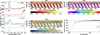 |
Fig. 3 (a) Mean and principal components computed using chopper.py and considering the PJ1 G21 subset. (b–d) Spatial maps of the first three principal components decomposition coefficients. (e) Cumulative PCA eigenvalues. |
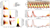 |
Fig. 4 (a) Results of the chopper.py GMM analysis on the PCA-decomposition coefficients presented in Fig. 3. The resulting clusters are represented using different colors in the corner plot of the distribution of the coefficients. (b) Spatial maps of the resulting PCA+GMM clusters found by chopper.py. (c) Mean spectra of the clusters found by chopper.py. (d) Same as panel c but the spectra are normalized for the radiance measured at 2.73 µm. |
4.2 Application to NIRSpec observations of the GRS
Figure 6 shows the results of the PCA analysis performed on the NIRSpec mosaic of the GRS. Also in this case, see Fig. 6f, more than 90% of the variance is captured using the first two principal components which still appear anticorrelated, as deduced by Irwin et al. (2001). In this case, our code found the first component to be correlated to the solar reflected signal, and the second to the thermal one. This is also visible in subpanels b,c,d, and e of Fig. 6, where the coefficients’ maps are presented. The first component map correlates to the solar reflected signal map presented in Fig. 1d. To reach a value larger than 95% in this case we need to use also the third and fourth eigenvectors. The physical interpretation of these components is not immediately clear. PC3 is similar in spectral shape and intensity to the PC3 derived in the case of the analysis of the JIRAM G21 subset, Fig. 3a. Therefore, we can extend the interpretation of PC3 obtained from JIRAM also to NIRSpec. On the other hand, looking at Fig. 6e, PC4 varies mostly in the dark filaments. Therefore it may be associated with variations in the spectral shape and intensity of the 4.4–4.7 µm region. We decided to retain only the first four components and therefore chopper.py performed the GMM clustering on the respective four-dimensional coefficients distribution. In this case, the elbow method suggests the best number of clusters to be four but we also tried to perform the clustering using five of them, as the difference in WCSS score between the two cases was small. Figure A.6 shows the PCA decomposition coefficient distributions and the result of the clustering analysis in the case of K=4. Figure 7 shows the PCA decomposition coefficient distributions and the result of the clustering analysis in the case of K=5. In both scenarios, our code can automatically identify and group together the spectra belonging to: the GRS (cluster 2, orange curves and points), the GRS hollow (cluster 1, dark red curves and points), the dark filaments that surround the GRS (cluster 3, green curves and points), and a transition zone between the hollow and the characteristic Jovian reddish-grayish regions (cluster 4, sky blue curves and points). Once again, the clustering of IR spectra returns results that correlate with the visible images.
In both cases, as pointed out in the previous subsection, the spectra associated with the dark filaments present the highest thermal signals, while the ones associated with the GRS have the highest solar reflected one. Therefore they tend to occupy opposite regions in the c1-c2 diagram, with the spectra of the GRS also emerging in the c2-c3 diagram. This underlines the consistency between the JIRAM and NIRSpec observations.
However, in the scenario with K=5 an additional group emerges without changing the distribution and shapes of the ones found in the K=4 scenario. This cluster seems to group a series of spectra that distribute geographically forming a halo that surrounds and include the outer rim of GRS. Differently from the other clusters, this halo is not evident from the optical HST or JunoCam images, and therefore they are unlikely to be related to differences in cloud optical depth and/or to the presence of chromophores (Carlson et al. 2016). If we consider the mean spectra, the solar reflected and thermal signals are almost identical. However, the mean spectrum of the halo presents a less broadened and distorted reflectance peak with respect to the mean spectrum of the inner GRS oval (see Fig. 7d). This may be caused by differences in altitude, vertical extension, particle effective radii, and/or composition. We will investigate this in the next section.
The detection of this halo highlights the fact that the use of PCA+GMM on IR spectral data is both useful to get global and mean physical properties of regions of interest known from visible images, but it also may lead to the detection of areas that are identifiable only at non-optical wavelengths.
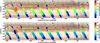 |
Fig. 5 Results derived from the atmospheric retrievals in the 2.5–3.1 µm range performed on the mean spectra presented in Fig. 4. In the top panel, the effective cloud altitude (see text for the definition) is represented, while in the bottom one the opacity scale height (see text for the definition). |
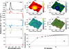 |
Fig. 6 (a) Mean and principal components computed considering the JWST/NIRSpec dataset. (b–e) Spatial maps of the first four principal components decomposition coefficients. (f) Cumulative PCA eigenvalues. |
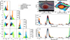 |
Fig. 7 (a) Results of the chopper.py GMM analysis on the PCA-decomposition coefficients presented in Fig. 6 using a value of K=5. The resulting clusters are represented using different colors in the corner plot of the distribution of the coefficients. (b and c) Spatial maps of the resulting PCA+GMM clusters found by chopper.py compared to HST images. (d) Mean spectra of the clusters found by chopper.py. (e) Same as panel d but the spectra are normalized for the radiance measured at 2.73 µm. |
4.3 Application to JIRAM PJ1 GRS subset
We applied our code also to the JIRAM observation of the GRS region during PJ1. The main goal is to verify whether the clustering analysis can identify the halo found using NIRSpec data, and under which combination of parameters. Figure 8 shows the obtained principal components. They are very similar - but not identical – to the ones presented in Fig. 3. Also in this case, the first component is correlated to the thermal signal, while the second correlates to the solar reflected one. The physical explanation of the third component is not trivial, and may be connected to intrinsic differences observed in the thermal spectra of the dark filaments, similarly to the PC4 derived in the NIRSpec case. The fourth component, instead, is almost identical to PC3 found in Fig. 3a and to PC3 found in Fig. 7a. Therefore it seems to be connected to second order effects in intensity and spectral shape induced by the presence of clouds and hazes. It can also be interpreted as a a correction for excessive/insufficient spectral broadening or reflection induced by PC2. More than 95% of variance is captured using only the first two components. However, since we suspected that the halo differs from the GRS because of cloud properties, we decided to perform the clustering twice: first using the c1 and c2 coefficients and then the c2 and c4 coefficients. In both scenarios, the elbow method suggested the best number of clusters to be four and we proceeded accordingly. The results of the clustering using only the decomposition coefficients relative to the first two components are given in Fig. A.7, while the results using the c2 and c4 coefficients are presented in Fig. 9. The first figure shows that when c1-c2 coefficients are used, chopper.py can automatically identify and group together the spectra belonging to the GRS, the hollow, the dark filaments, and the surroundings. In the end, we found the same results of the G21 subset, as the c1-c2 coefficients are practically identical. However, even if K>4 clusters are used, the code is not able to detect any halos surrounding the GRS inner oval. When c2-c4 coefficients are used, the spectra belonging to the inner GRS oval and the halo easily emerge and they are grouped by the code. This underlines the fact that clustering can be very powerful also if one can identify principal components of interest from a physical point of view. Therefore chopper.py can be used both in an unsupervised or supervised fashion, depending on the scientific case of interest. It is worth to underline that in the case of identifying the halo in JIRAM data a supervised approach in the form of a selection of the PCA coefficients parameter space is mandatory. In fact, as the first two PCs capture more than 95% of the variance they also dominate the clustering process. This is not true in the JWST case because of the higher spectral and spatial resolution of NIRSpec. Therefore, as the spectra of the halo and of the inner oval seems to exhibit similar solar and thermal signals, they can never be disentangled in the PC1-PC2 space.
The spectra of the hollow and the dark filaments are grouped in one cluster as they both belong to the SEB, while the remaining group joins together the spectra belonging to the EZ and the STrZ. The coefficients of the halo and the inner GRS occupy a very distinct space in the c2-c4 parameter space with respect to the coefficients of the GRS surroundings region. This is consistent with the GRS having clouds different from the other Jovian regions, both in composition, vertical distribution, and dynamical origin. Noteworthy, the coefficients of the halo seem to occupy a transition zone between the typical Jovian clouds and the GRS ones, and this is perhaps the reason why it was not possible to detect the halo from the visible images. Also in the JIRAM case, the mean spectra of the GRS and the halo have similar solar and thermal radiation levels. The JIRAM mean spectrum of the halo presents a less broadened and distorted reflectance peak with respect to the JIRAM mean spectrum of the inner GRS oval.
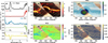 |
Fig. 8 (a) Mean and principal components computed considering the Juno/JIRAM PJ1 GRS subset. (b–e) Spatial maps of the first four principal components decomposition coefficients. |
5 Discussion: Identification of the GRS “halo”
The main conclusion of our PCA+GMM clustering is the detection of a group of spectral pixels that seem to form a halo corresponding to the outer rim of the GRS, Fig. 11. The GRS inner oval pixels on the other hand were classified in a different cluster. The mean spectra extracted from the halo and the inner GRS oval have the same values for solar-reflected and thermal emitted radiation. However, they differ principally in the shape of the 2.73 µm reflection peak, see Fig. 10, which for the inner GRS appears to be more broadened with respect to the halo. The detection was made using both JWST/NIRSpec and Juno/JIRAM data. In the case of JWST/NIRSpec, the detection was completely unsupervised. For Juno/JIRAM, we needed to follow a supervised approach and select manually the PCA coefficients parameter space on which the clustering was performed. While the GRS appears quite uniform from visible and NIR maps (see Figs. 11a and 11b), the IR spectra suggest that the GRS is not uniform but consists of two main concentric structures. This is evident from the radiance maps at wavelengths where both solar and thermal contributions become important, like the 4.5 µm channel (see Fig. 11c).
While the presence of rings or bright regions around the outer rim of Jovian anticyclones was noted before at 5 µm (de Pater et al. 2010) and radio wavelengths (de Pater et al. 2016, 2019b,a) the halo detected here is interior to these rings, see Fig. 11d and has not been detected before. de Pater et al. (2010) proposed that air is (baroclinically) rising along the center of Jovian anticyclones in a subadiabatic atmosphere, then descending at a distance not exceeding twice the local Rossby deformation radius. For the GRS, they proposed that the air rises in a ring around the center of the GRS, descending inside that ring (explaining the slight elevation in temperature at the center of the GRS, observed by Fletcher et al. 2010) and presumably also outside that ring.
As the visible images and the NIR maps in Fig. 11b do not suggest the presence of two main concentric structures inside the GRS, we suspect that the halo and the inner oval share the same chromophore upper layer in the Crème Brûlée model (Baines et al. 2019; Carlson et al. 2016) and similar 1-bar cumulative optical depth values. The broadening of the 2.73 µm reflection peak is a hint that the main difference between the halo and the inner oval may lie in the vertical extension of the main cloud layer, and therefore in the pressure level at which a value of 1 in optical depth is reached in the upper troposphere.
To verify this hypothesis, we run different forward simulations using the NEMESIS radiative transfer suite (Irwin et al. 2008), focusing on the 2.5–3.2 µm range. The spectral database, the abundances of H2, He, CH4, and its isotopologues are the same as those described in Harkett et al. (2024). We assumed Voigt broadening for all wavelengths with a line wing cut-off of 350 cm−1 generating pre-tabulated k-ditributions using the spectral range and resolution of the NIRSpec instrument. The pressure-temperature profile was fixed to the one measured by Cassini/CIRS (Fletcher et al. 2009). NH3 and PH3 gaseous volume mixing ratio (VMR) profiles have a fixed single value from a “knee” pressure and extend down to 10 bar. At altitudes above the knee pressure, the profiles decrease with a Fractional Scale Height (FSH). We decided to fix the ammonia knee pressure at 860 mbar, and the phosphine knee pressure at 500 mbar, according to Harkett et al. (2024). We use a value of 230 ppm for the NH3 deep VMR, and of 0.8 ppm for PH3 deep VMR, as derived from the MIRI data (Harkett et al. 2024). The chosen FSH are 0.13 for ammonia and 0.25 for phosphine.
The main ingredient of our forward simulations is the aerosols. In the NIRSpec range we are not sensitive to any tropospheric or stratospheric blue-absorbing species like the Carlson et al. (2016) and Baines et al. (2019) chromophores. The Jovian spectrum in the NIR, in fact, is more sensitive to the main cloud layer that lies below the chromophore layer. The work of Grassi et al. (2021) and Biagiotti et al. (2025) have shown that tholins are a good approximation for the optical properties of the unknown material that compose the Jovian clouds. We therefore used Imanaka et al. (2012) tholins with optical properties computed using Mie theory for spherical particles of 2 µm radius. We used three different cloud profiles to perform the forward simulation, as shown in Fig. 12 panel a. They are represented by a base pressure level, an optical depth normalized at 2.73 µm, and a cloud fractional scale height. All the profiles have a base pressure level of 2 bar (Irwin et al. 2025), consistent with Baines et al. (2019). The optical depth is adjusted manually to make it so that all the profiles have a cumulative optical depth at 1.2 bar (panel b) equal to five, consistent with Braude et al. (2020). This is also consistent with the observed solar and thermal signal values of the halo and the inner GRS. The only variable that discriminates between the profiles is the fractional scale height (CFSH). The green profile has a CFSH=0.4, the violet profile a CFSH=0.55, and the pink profile a CFSH=0.7. A larger CSFH translates in a larger vertical extension of the cloud layer, i.e. more cloud particles at higher altitudes. It is possible to note this from Fig. 12b, where the cumulative optical depths are shown. As a consequence, the profiles with larger CFSH reach a value of unity in optical depth higher in the troposphere (at lower pressures). In Table A.3 we resume the used parameters for each NEMESIS simulation. The results of the NEMESIS simulations are presented in 12 panel c. We draw two main conclusions from Fig. 12. The first is that NEMESIS used together with tholin-like clouds can reproduce quite well the spectral shape observed by NIRSpec in the 2.5–3.1 µm range. Secondly, a difference in cloud fractional scale height (and therefore in cloud vertical extension) can explain the broadening of the solar reflection peak observed with NIRSpec. This in turn may suggest that clouds closer to the center of the GRS at the time of the NIRSpec observations were reaching higher altitudes than the ones near the outer rim. Therefore, the halo detected with NIRSpec may be a consequence of increasing transparency of the GRS aerosols with radial distance. In other words, the halo can be a region where reflection from the deeper clouds is blending with the chromophore layer. This would be consistent with some optical and UV HST images, where the colour and the measured radiances change subtly towards the GRS edge and are more intense at the center (Simon et al. 2024).
Quantitatively, NEMESIS simulations suggest that between the center of the GRS and its outer rim may exist a difference in altitude of 10–20 km regarding the level at which the clouds become optically thick. These kinds of differences in altitude are consistent with recent fluid dynamics simulations by Zhang & Marcus (2024) for which a “spinning-top”-like shape for the GRS should be more stable than the classical cylinder shape proposed previously in literature (Parisi et al. 2021). Moreover, the formation of higher clouds is highly favored by the low temperatures found in the GRS inner oval (Fletcher et al. 2010; Harkett et al. 2024).
In any case, the modeling of a cloudy atmosphere is a very degenerate task. This means that similar variations in the resulting synthetic spectrum can be obtained with different combinations of the input parameters. Therefore, multiple scattering atmospheric retrievals of the NIRSpec spectra over a broader spectral range (to break some of these degeneracies) are needed to verify the hypothesis presented in this paper and to obtain quantitative results. However, this is beyond the scope of the present analysis.
The halo spectral cluster seems to align closely with the outer edge of the GRS red ellipse in visible-wavlength HST data (see panels b and c in Fig. 7). This location is close to two key features of the velocity field of the vortex: the high-speed ring of maximum azimuthal velocities, and the associated region of cyclonic shielding (Valcke & Verron 1997; Brueshaber et al. 2019; Li et al. 2020) just outside this high-speed ring. An accurate comparison between the position of the halo spectral cluster and specific velocity field features is not possible because the GRS velocity field is variable on both short and long timescales (Wong et al. 2021; Simon et al. 2024), but the wind field was not measured at the time of the JWST/NIRSpec observations nor the JIRAM PJ1 observations. The edge of the visible red area of the GRS and Oval BA typically lies just outside the high-speed ring (Wong et al. 2011; Simon et al. 2024), with the cyclonic shielding just outside the high-speed ring (Wong et al. 2021). Thus the halo spectral cluster may align better with the cyclonic shielding region of the velocity field, which is qualitatively consistent with the reduced cloud opacity interpretation, because cyclonic shear is often associated with subsidence, warming, and evaporation/sublimation of cloud material. Future observations with simultaneous near-IR resolved spectra and visible-wavelength velocity fields are needed for a detailed comparison.
Lastly, we note that the analysis of the NIRSpec data did not give any evidence of a GRS tilt as observed by Harkett et al. (2024). The distribution of clusters in Fig. 7 doesn’t give any indication of a tilt in the cloud properties. However, no correlation was found between clusters and the distribution of NH3 and PH3, nor any principal component spectra correlated with their absorption features, possibly as the approach focusses on the broad-band differences in shape, rather than narrow-band differences in the absorptions of gases. Therefore, in order to investigate the presence of a GRS tilt in NIRSpec data it is mandatory to overcome the influence of clouds and multiple scattering. This can be done focusing on narrower spectral intervals, surrounding NH3 and PH3 absorption features.
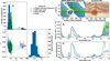 |
Fig. 9 (a) Results of the chopper.py GMM analysis on the second and fourth PCA-decomposition coefficients presented in Fig. 8. The resulting clusters are represented using different colors in the corner plot of the distribution of the coefficients, (b and c) Spatial maps of the resulting PCA+GMM clusters found by chopper.py compared to JunoCam image, (d) Mean spectra of the clusters found by chopper.py. (e) Same as panel d but the spectra are normalized for the radiance measured at 2.73 µm. |
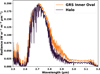 |
Fig. 10 JWST/NIRSpec mean spectrum of the inner GRS oval (orange) and of the halo (burgundy) found thanks to the chopper.py code. |
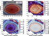 |
Fig. 11 Contours of the of the inner GRS oval (orange) and of the halo (burgundy) clusters identified in Fig. 7 superimposed to: (a) HST visible image, (b–d) NIRSpec radiance maps at respectively 2.7, 4.5, and 5 µm. |
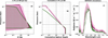 |
Fig. 12 (a) Cloud profiles (given as 2.73 µm optical depth per bar) of the three different model atmospheres used to perform NEMESIS simulations, (b) computed cumulative 2.73 µm optical depth for each of the model atmospheres, (c) NEMESIS simulations of three different model atmospheres that differ for the vertical extension of the main cloud layer. |
6 Summary
In this work, we present a new simple approach to grouping similar spectra that belong to a random collection into different clusters. We developed a Python code that first performs a PCA and decomposition, followed by an unsupervised clustering of self-similar spectra using GMMs. The core concept behind the code is to associate each spectrum in the dataset with a series of PCA decomposition coefficients to facilitate the clustering step. The code only retains the principal components that explain more than 95% of the original dataset variance. The number of clusters is a free parameter and can be either selected by the user or automatically derived using the elbow method.
We applied the code to two different subsets of JIRAM PJ1 data: (i) a subset of the data already analyzed in Grassi et al. (2021) and (ii) a close-up view of the GRS. We also applied the code to the mosaics of the GRS region acquired by NIR-Spec with the G235H and G395H gratings. Both the JIRAM and JWST data have been previously corrected for the presence of spikes or missing values induced by saturation (King et al. 2023). The results can be summarized as follows:
The PCA+GMM analysis can greatly improve the efficiency in the multiple scattering atmospheric retrieval stage by reducing the number of spectra to be inverted. To verify this, we performed a multiple scattering atmospheric retrieval for each of the five mean cluster spectra obtained by analyzing the G21 subset. We then derived quantized maps of cloud properties and compared them to the ones obtained by Grassi et al. (2021), who performed a retrieval for each of the 11 000+ spectra in the dataset. The agreement between the maps is good, both quantitatively and qualitatively. These kinds of analyses could prove useful for future planetary-oriented missions such as JUICE (Fletcher et al. 2023) or ARIEL (Tinetti et al. 2018).
A PCA+GMM analysis of IR data can automatically group spectra belonging to regions of interest identified in visible images. This was demonstrated through the analysis of both JIRAM and NIRSpec datasets. In the case of the JIRAM data, the method was able to automatically group the spectra belonging to: the GRS, the STrZ, the STB, and the different regions in cloud opacity comprising the SEB. In the case of NIRSpec data, the code autonomously grouped together the spectra belonging to: the GRS, the GRS’ hollow, the dark filaments in the wake, and in the surroundings.
A PCA+GMM analysis of IR data can automatically group spectra belonging to regions of interest that are not seen in visible images. This was made evident when analyzing NIRSpec data. Using five clusters, the code was able to identify two concentric structures in the GRS: a halo that corresponded to the pixels of the outer rim of the GRS, and an inner red oval. The mean spectra of the halo and the inner GRS oval presented similar values of the observed solar (2.73 µm) and thermal (>4.6 µm) radiances. However, the mean spectrum of the inner GRS oval presents a more broadened solar-reflected peak with respect to the mean spectrum of the halo. The same concentric structures have also been detected in JIRAM data. In that case, however, the halo emerges only if the decomposition coefficients of the principal components connected to cloud properties are used during the clustering stage. In both the cases, the halo seems to be interior the bright IR and radio rings (de Pater et al. 2010).
Guided by the results of a series of NEMESIS simulations, we propose that the main difference between the halo and the inner GRS oval is likely the vertical extension of the main cloud decks. We also suggest that the detection of both the halo and an inner oval inside the GRS may be the consequence of increasing transparency of the GRS aerosols with radial distance. This is supported by the observed values in radiances in the halo and the inner oval, which suggest that the base pressure levels and optical depth values could be quite similar. Moreover, the optical images do not show differences in the red channel that lead to the presence of different chromophores. This hypothesis would be consistent with the fluid dynamics simulations of Zhang & Marcus (2024). However, we stress that multiple scattering atmospheric retrievals using the entire spectral range offered by JIRAM and NIRSpec are needed to verify or reject our hypothesis.
Data availability
Part of the data underlying this article are available in NASA Planetary Data System at https://pds-atmospheres.nmsu.edu/data_and_services/atmospheres_data/JUNO/jiram.html.
The chopper.py code is made available both on GitHub and Zenodo at the following links: https://github.com/astro-francy/chopper, and https://doi.org/1S.5281/zenodo.15731419
Acknowledgements
Part of this work is based on observations made with the NASA/ESA/CSA James Webb Space Telescope. The data were obtained from the Mikulski Archive for Space Telescopes (MAST) at the Space Telescope Science Institute (STScl), which is operated by the Association of Universities for Research in Astronomy, Inc. (AURA), under NASA contracts NAS 5-03127 for JWST and NAS 5-26555 for HST. The JWST observations in this paper are associated with program #1373, which is led by co-PIs Imke de Pater and Thierry Fouchet. JIRAM is supported by the Italian Space Agency (ASI). This work is funded by the Addendum N. 2016-23-H.3-2023 to the ASI-INAF Agreement N. 2016-23-H.0. Part of the research activities described in this paper were carried out with contribution of the Next Generation EU funds within the National Recovery and Resilience Plan (PNRR), Mission4 - Education and Research, Component 2 - From Research to Business (M4C2), Investment Line 3.1 Strengthening and creation of Research Infrastructures, Project IR0000038 – “Earth Moon Mars (EMM)”. EMM is led by INAF in partnership with ASI and CNR. Figures 7b and 11a are based on observations associated with program GO-16913, made with the NASA/ESA Hubble Space Telescope, obtained from MAST at STScI. Support for GO-16913 was provided by STScI to M.H.W. and G.S.O. M.H.W. was also supported by NASA Juno Participating Scientist grant 80NSSC19K1265. F.B. acknowledges the Ph.D. course in Astronomy, Astrophysics and Space Science of the University of Rome “Sapienza”, University of Rome “Tor Vergata” and INAF, Italy. Fletcher, Roman, and King are supported by STFC Consolidated Grant reference ST/W00089/X1. H.M. was supported by a STFC James Webb Fellowship (ST/W001527/2) at Northumbria University. G.S.O. is supported by funds from NASA distributed to the Jet Propulsion Laboratory, California Institute of Technology under a contract (80NM0018D0004). I.d.P. and M.H.W. are in part supported by the Space Telescope Science Institute grant nr. JWST-ERS-01373. R.H. is supported by grant PID2023-149055NB-C31 funded by MICIU/AEI/10.13039/501100011033 and FEDER, UE; and by Grupos Gobierno Vasco IT1742-22. JIRAM has been developed by Leonardo S.p.A. at the Officine Galileo – Campi Bisenzio site. We thank the anonymous referee for their careful reading and thoughtful comments that have greatly improved the paper. F.B. thanks E. Giancarli, F.P. Ramunno, S. Mestici, F. Colaiuta, and S. Rubino for the helpful discussions about chopper.py. The JIRAM instrument was conceived and brought to reality by our late collaborator and institute Director Dr. Angioletta Coradini (1946–2011).
Appendix A Supplementary materials
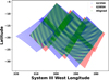 |
Fig. A.1 Manual alignement performed to combine the G235H and G395H NIRSpec mosaics. |
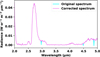 |
Fig. A.2 Example of a JIRAM spectrum in the G21 subset before (cyan) and after (orchid) being corrected for the presence of spikes. |
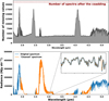 |
Fig. A.3 Top panel: Wavelength distribution of missing values in the Jovian spectra collected by JWST/NIRSpec. Bottom panel: Example of an original NIRSpec spectrum (blue) and the correction made to perform an accurate and unbiased PCA+GMM analysis (orange). Zoom-in panel shows the results of the applied imputation methods for missing values. |
Employed data cleaning procedures for JIRAM and NIRSpec.
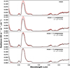 |
Fig. A.4 Example of the results of the PCA decomposition (black curves, at various stages), cf. Eqn. (1), applied to a random spectrum of the PJ1 G21 subset (red curve). The quality of the reconstruction after the decomposition is given by the parameter 1 −χ2, which should be close to unity. |
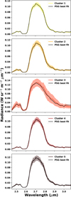 |
Fig. A.5 Results of the PSG multiple scattering retrievals performed on the five cluster mean spectra identified in Fig. 3. |
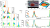 |
Fig. A.6 (a) Results of the chopper.py GMM analysis on the PCA-decomposition coefficients presented in Fig. 6 using a value of K=4. The resulting clusters are represented using different colors in the corner plot of the distribution of the coefficients. (b and c) Spatial maps of the resulting PCA+GMM clusters found by chopper.py compared to HST images. (d) Mean spectra of the clusters found by chopper.py. (e) Same as panel d but the spectra are normalized for the radiance measured at 2.73 µm. |
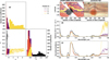 |
Fig. A.7 (a) Results of the chopper.py GMM analysis on the first and second PCA-decomposition coefficients presented in Fig. 8. The resulting clusters are represented using different colors in the corner plot of the distribution of the coefficients. (b) Spatial maps of the resulting PCA+GMM clusters found by chopper.py. (c) Mean spectra of the clusters found by chopper.py. (d) Same as panel c but the spectra are normalized for the radiance measured at 2.73 µm. |
References
- Adriani, A., Filacchione, G., Di Iorio, T., et al. 2017, Space Sci. Rev., 213, 393 [NASA ADS] [CrossRef] [Google Scholar]
- Adriani, A., Mura, A., Orton, G., et al. 2018, Nature, 555, 216 [NASA ADS] [CrossRef] [Google Scholar]
- Anguiano-Arteaga, A., Pérez-Hoyos, S., Sánchez-Lavega, A., Sanz-Requena, J. F., & Irwin, P. G. J. 2021, J. Geophys. Res., 126, e06996 [Google Scholar]
- Anguiano-Arteaga, A., Pérez-Hoyos, S., Sánchez-Lavega, A., Sanz-Requena, J. F., & Irwin, P. G. J. 2023, J. Geophys. Res. Planets, 128, e2022JE007427 [Google Scholar]
- Ardévol Martínez, F., Min, M., Huppenkothen, D., Kamp, I., & Palmer, P. I. 2024, A&A, 681, L14 [NASA ADS] [CrossRef] [EDP Sciences] [Google Scholar]
- Atreya, S. K., Wong, A. S., Baines, K. H., Wong, M. H., & Owen, T. C. 2005, Planet. Space Sci., 53, 498 [Google Scholar]
- Baines, K. H., Sromovsky, L. A., Carlson, R. W., Momary, T. W., & Fry, P. M. 2019, Icarus, 330, 217 [Google Scholar]
- Bandfield, J. L., Hamilton, V. E., & Christensen, P. R. 2000, Science, 287, 1626 [CrossRef] [Google Scholar]
- Baumeister, P., Padovan, S., Tosi, N., et al. 2020, ApJ, 889, 42 [Google Scholar]
- Biagiotti, F. 2025, https://doi.org/10.5281/zenodo.15731420 [Google Scholar]
- Biagiotti, F., Grassi, D., Liuzzi, G., et al. 2025, MNRAS, 538, 1535 [Google Scholar]
- Bolton, S. J., Adriani, A., Adumitroaie, V., et al. 2017a, Science, 356, 821 [Google Scholar]
- Bolton, S. J., Lunine, J., Stevenson, D., et al. 2017b, Space Sci. Rev., 213, 5 [CrossRef] [Google Scholar]
- Braude, A. S., Irwin, P. G. J., Orton, G. S., & Fletcher, L. N. 2020, Icarus, 338, 113589 [Google Scholar]
- Brueshaber, S. R., Sayanagi, K. M., & Dowling, T. E. 2019, Icarus, 323, 46 [Google Scholar]
- Brzycki, B., Siemion, A. P. V., Croft, S., et al. 2020, PASP, 132, 114501 [Google Scholar]
- Campello, R. J. G. B., Moulavi, D., & Sander, J. 2013, in Advances in Knowledge Discovery and Data Mining, eds. J. Pei, V. S. Tseng, L. Cao, H. Motoda, & G. Xu (Berlin, Heidelberg: Springer), 160 [Google Scholar]
- Carlson, R. W., Baines, K. H., Anderson, M. S., Filacchione, G., & Simon, A. A. 2016, Icarus, 274, 106 [Google Scholar]
- Christensen, P. R., Bandfield, J. L., Hamilton, V. E., et al. 2001, J. Geophys. Res., 106, 23823 [Google Scholar]
- Christensen, P. R., Jakosky, B. M., Kieffer, H. H., et al. 2004, Space Sci. Rev., 110, 85 [Google Scholar]
- de Pater, I., Wong, M. H., Marcus, P., et al. 2010, Icarus, 210, 742 [Google Scholar]
- de Pater, I., Sault, R. J., Butler, B., DeBoer, D., & Wong, M. H. 2016, Science, 352, 1198 [Google Scholar]
- de Pater, I., Sault, R. J., Moeckel, C., et al. 2019a, AJ, 158, 139 [Google Scholar]
- de Pater, I., Sault, R. J., Wong, M. H., et al. 2019b, Icarus, 322, 168 [Google Scholar]
- Dyudina, U. A., Ingersoll, A. P., Danielson, G. E., et al. 2001, Icarus, 150, 219 [Google Scholar]
- Ellis, R. S., Bland-Hawthorn, J., Bremer, M., et al. 2017, arXiv e-prints [arXiv:1701.01976] [Google Scholar]
- Enriquez, J. E., Siemion, A., Foster, G., et al. 2017, ApJ, 849, 104 [CrossRef] [Google Scholar]
- Ester, M., Kriegel, H.-P., Sander, J., & Xu, X. 1996, in Second International Conference on Knowledge Discovery and Data Mining (KDD’96). Proceedings of a conference held August 2-4, eds. D. W. Pfitzner, & J. K. Salmon, 226 [Google Scholar]
- Fletcher, L. N., Orton, G. S., Teanby, N. A., & Irwin, P. G. J. 2009, Icarus, 202, 543 [NASA ADS] [CrossRef] [Google Scholar]
- Fletcher, L. N., Orton, G. S., Mousis, O., et al. 2010, Icarus, 208, 306 [CrossRef] [Google Scholar]
- Fletcher, L. N., Cavalié, T., Grassi, D., et al. 2023, Space Sci. Rev., 219, 53 [Google Scholar]
- Fletcher, L. N., Biagiotti, F., King, O. R. T., et al. 2024, in European Planetary Science Congress, EPSC2024-801 [Google Scholar]
- Gajjar, V., LeDuc, D., Chen, J., et al. 2022, ApJ, 932, 81 [Google Scholar]
- Gardner, J. P., Mather, J. C., Clampin, M., et al. 2006, Space Sci. Rev., 123, 485 [Google Scholar]
- Goldberger, J., Hinton, G. E., Roweis, S., & Salakhutdinov, R. R. 2004, in Advances in Neural Information Processing Systems, eds. L. Saul, Y. Weiss, & L. Bottou (Cambridge: MIT Press), 17 [Google Scholar]
- Grassi, D., Mura, A., Sindoni, G., et al. 2021, MNRAS, 503, 4892 [NASA ADS] [CrossRef] [Google Scholar]
- Grassi, D., Mura, A., Adriani, A., et al. 2024, MNRAS, 533, 2185 [Google Scholar]
- Harkett, J., Fletcher, L. N., King, O. R. T., et al. 2024, J. Geophys. Res. Planets, 129, e2024JE008415 [Google Scholar]
- Hayes, J. J. C., Kerins, E., Awiphan, S., et al. 2020, MNRAS, 494, 4492 [NASA ADS] [CrossRef] [Google Scholar]
- Horton, D. E., Johnson, N. C., Singh, D., et al. 2015, Nature, 522, 465 [Google Scholar]
- Imanaka, H., Cruikshank, D. P., Khare, B. N., & McKay, C. P. 2012, Icarus, 218, 247 [NASA ADS] [CrossRef] [Google Scholar]
- Irwin, P. G. J., & Dyudina, U. 2002, Icarus, 156, 52 [Google Scholar]
- Irwin, P. G. J., Weir, A. L., Smith, S. E., et al. 1998, J. Geophys. Res., 103, 23001 [NASA ADS] [CrossRef] [Google Scholar]
- Irwin, P. G. J., Weir, A. L., Taylor, F. W., Calcutt, S. B., & Carlson, R. W. 2001, Icarus, 149, 3974 [Google Scholar]
- Irwin, P. G. J., Teanby, N. A., de Kok, R., et al. 2008, J. Quant. Spec. Radiat. Transf., 109, 1136 [NASA ADS] [CrossRef] [Google Scholar]
- Irwin, P. G. J., Hill, S. M., Fletcher, L. N., Alexander, C., & Rogers, J. H. 2025, J. Geophys. Res. Planets, 130, 2024JE008622 [Google Scholar]
- Ivezic, Ž., Connolly, A. J., VanderPlas, J. T., & Gray, A. 2014, Statistics, Data Mining, and Machine Learning in Astronomy: A Practical Python Guide for the Analysis of Survey Data (Princeton: Princeton University Press) [Google Scholar]
- Jain, A. K. 2010, Pattern Recog. Lett., 31, 651 [Google Scholar]
- Jakobsen, P., Ferruit, P., Alves de Oliveira, C., et al. 2022, A&A, 661, A80 [NASA ADS] [CrossRef] [EDP Sciences] [Google Scholar]
- Kalogerakis, K. S., Marschall, J., Oza, A. U., et al. 2008, Icarus, 196, 202 [Google Scholar]
- Kelly, B. C. 2007, ApJ, 665, 1489 [Google Scholar]
- King, O. R. T., Fletcher, L. N., Harkett, J., Roman, M. T., & Melin, H. 2023, Res. Notes Am. Astron. Soc., 7, 223 [Google Scholar]
- Lebofsky, M., Croft, S., Siemion, A. P. V., et al. 2019, PASP, 131, 124505 [NASA ADS] [CrossRef] [Google Scholar]
- Leon-Dasi, M., Besse, S., & Doressoundiram, A. 2023, Remote Sens., 15, 4560 [Google Scholar]
- Li, C., Ingersoll, A., Janssen, M., et al. 2017, Geophys. Res. Lett., 44, 5317 [CrossRef] [Google Scholar]
- Li, C., Ingersoll, P., A., Klipfel, P., A., & Brettle, H. 2020, Proc. Natl. Acad. Sci., 117, 24082 [Google Scholar]
- Ma, P. X., Ng, C., Rizk, L., et al. 2023, Nat. Astron., 7, 492 [NASA ADS] [Google Scholar]
- Maahn, M., Turner, D. D., Löhnert, U., et al. 2020, Bull. Am. Meteorol. Soc., 101, E1512 [Google Scholar]
- Malin, M. C., & Edgett, K. S. 2001, J. Geophys. Res., 106, 23429 [Google Scholar]
- Malin, M. C., Bell, J. F., Cantor, B. A., et al. 2007, J. Geophys. Res. Planets, 112, E05S04 [Google Scholar]
- McEwen, A. S., Eliason, E. M., Bergstrom, J. W., et al. 2007, J. Geophys. Res. Planets, 112, E05S02 [Google Scholar]
- Melin, H., O’Donoghue, J., Moore, L., et al. 2024, Nat. Astron., 8, 1000 [Google Scholar]
- Moon, T. K. 1996, IEEE Signal Process. Mag., 13, 47 [Google Scholar]
- Mura, A., Adriani, A., Connerney, J. E. P., et al. 2018, Science, 361, 774 [Google Scholar]
- Murchie, S., Arvidson, R., Bedini, P., et al. 2007, J. Geophys. Res. Planets, 112, E05S03 [Google Scholar]
- Mustard, J. F., Murchie, S. L., Pelkey, S. M., et al. 2008, Nature, 454, 305 [Google Scholar]
- Niemann, H. B., Atreya, S. K., Carignan, G. R., et al. 1996, Science, 272, 846 [CrossRef] [Google Scholar]
- Nixon, M. C., & Madhusudhan, N. 2020, MNRAS, 496, 269 [NASA ADS] [CrossRef] [Google Scholar]
- Ordonez-Etxeberria, I., Hueso, R., Sánchez-Lavega, A., & Pérez-Hoyos, S. 2016, Icarus, 267, 34 [Google Scholar]
- Parisi, M., Kaspi, Y., Galanti, E., et al. 2021, Science, 374, 964 [NASA ADS] [CrossRef] [Google Scholar]
- Pearson, K. 1901, London Edinburgh Dublin Phil. Mag. J. Sci., 2, 559 [CrossRef] [Google Scholar]
- Pedregosa, F., Varoquaux, G., Gramfort, A., et al. 2011, J. Mach. Learn. Res., 12, 2825 [Google Scholar]
- Rodgers, C. D. 2000, Inverse Methods for Atmospheric Sounding: Theory and Practice (Singapore: World Scientific) [Google Scholar]
- Sagan, C., & Khare, B. N. 1979, Nature, 277, 102 [Google Scholar]
- Sanchez-Lavega, A., Orton, G. S., Morales, R., et al. 2001, Icarus, 149, 491 [Google Scholar]
- Sánchez-Lavega, A., García-Melendo, E., Legarreta, J., et al. 2024, Geo-phys. Res. Lett., 51, e2024GL108993 [Google Scholar]
- Simon, A. A., Wong, M. H., Marcus, P. S., & Irwin, P. G. J. 2024, Planet. Sci. J., 5, 223 [Google Scholar]
- Simon-Miller, A. A., Banfield, D., & Gierasch, P. J. 2001, Icarus, 154, 459 [Google Scholar]
- Sromovsky, L. A., & Fry, P. M. 2010a, Icarus, 210, 211 [Google Scholar]
- Sromovsky, L. A., & Fry, P. M. 2010b, Icarus, 210, 230 [Google Scholar]
- Tinetti, G., Drossart, P., Eccleston, P., et al. 2018, Exp. Astron., 46, 135 [NASA ADS] [CrossRef] [Google Scholar]
- Valcke, S., & Verron, J. 1997, J. Phys. Oceanography, 27, 524 [Google Scholar]
- VanderPlas, J., Connolly, A. J., Ivezic, Z., & Gray, A. 2012, in Proceedings of Conference on Intelligent Data Understanding (CIDU), 47 [Google Scholar]
- VanderPlas, J., Fouesneau, M., & Taylor, J. 2014, Astrophysics Source Code Library [record ascl:1407.018] [Google Scholar]
- Villanueva, G. L., & Milam, S. N. 2023, Nat. Commun., 14, 7444 [Google Scholar]
- Villanueva, G. L., Smith, M. D., Protopapa, S., Faggi, S., & Mandell, A. M. 2018, J. Quant. Spec. Radiat. Transf., 217, 86 [NASA ADS] [CrossRef] [Google Scholar]
- Virtanen, P., Gommers, R., Oliphant, T. E., et al. 2020, Nat. Methods, 17, 261 [Google Scholar]
- von Zahn, U., Hunten, D. M., & Lehmacher, G. 1998, J. Geophys. Res., 103, 22815 [NASA ADS] [CrossRef] [Google Scholar]
- Waldmann, I. P., & Griffith, C. A. 2019, Nat. Astron., 3, 620 [Google Scholar]
- Whitaker, D. A., & Hayes, K. 2018, Chemomet. Intell. Lab. Syst., 179, 82 [Google Scholar]
- Wong, M. H., Mahaffy, P. R., Atreya, S. K., Niemann, H. B., & Owen, T. C. 2004, Icarus, 171, 153 [Google Scholar]
- Wong, M. H., de Pater, I., Asay-Davis, X., Marcus, P. S., & Go, C. Y. 2011, Icarus, 215, 211 [NASA ADS] [CrossRef] [Google Scholar]
- Wong, M. H., Marcus, P. S., Simon, A. A., et al. 2021, Geophys. Res. Lett., 48, e93982 [Google Scholar]
- Wong, M. H., Bjoraker, G. L., Goullaud, C., et al. 2023, Remote Sens., 15, 702 [Google Scholar]
- Yang, H., Shi, C., Cai, J., et al. 2022, MNRAS, 517, 5496 [NASA ADS] [CrossRef] [Google Scholar]
- Zhang, A., & Marcus, P. S. 2024, J. Fluid Mech., 984, A61 [Google Scholar]
- Ziv, M., Galanti, E., Howard, S., Guillot, T., & Kaspi, Y. 2024a, A&A, 692, A251 [NASA ADS] [CrossRef] [EDP Sciences] [Google Scholar]
- Ziv, M., Galanti, E., Sheffer, A., et al. 2024b, A&A, 686, L7 [NASA ADS] [CrossRef] [EDP Sciences] [Google Scholar]
All Tables
All Figures
|
Fig. 1 (a) Spatial distribution of all the JIRAM PJ1 collected and non-corrupted spectra. (b) Spatial map of radiance measured at 2.73 µm for the G21 susbset of PJ1 data considered in this work. (c) Spatial map of radiance measured at 2.73 µm for the GRS susbset of PJ1 data. (d) Spatial maps of radiance measured by JWST/NIRSpec at 2.73 µm. |
| In the text | |
|
Fig. 2 Comparison between two spectra of the GRS captured, respectively, by Juno/JIRAM (top panel) and JWST/NIRSpec (bottom panel). It is possible to note the higher spectral resolution of NIRSpec, which must not be confused with noise. |
| In the text | |
|
Fig. 3 (a) Mean and principal components computed using chopper.py and considering the PJ1 G21 subset. (b–d) Spatial maps of the first three principal components decomposition coefficients. (e) Cumulative PCA eigenvalues. |
| In the text | |
|
Fig. 4 (a) Results of the chopper.py GMM analysis on the PCA-decomposition coefficients presented in Fig. 3. The resulting clusters are represented using different colors in the corner plot of the distribution of the coefficients. (b) Spatial maps of the resulting PCA+GMM clusters found by chopper.py. (c) Mean spectra of the clusters found by chopper.py. (d) Same as panel c but the spectra are normalized for the radiance measured at 2.73 µm. |
| In the text | |
|
Fig. 5 Results derived from the atmospheric retrievals in the 2.5–3.1 µm range performed on the mean spectra presented in Fig. 4. In the top panel, the effective cloud altitude (see text for the definition) is represented, while in the bottom one the opacity scale height (see text for the definition). |
| In the text | |
|
Fig. 6 (a) Mean and principal components computed considering the JWST/NIRSpec dataset. (b–e) Spatial maps of the first four principal components decomposition coefficients. (f) Cumulative PCA eigenvalues. |
| In the text | |
|
Fig. 7 (a) Results of the chopper.py GMM analysis on the PCA-decomposition coefficients presented in Fig. 6 using a value of K=5. The resulting clusters are represented using different colors in the corner plot of the distribution of the coefficients. (b and c) Spatial maps of the resulting PCA+GMM clusters found by chopper.py compared to HST images. (d) Mean spectra of the clusters found by chopper.py. (e) Same as panel d but the spectra are normalized for the radiance measured at 2.73 µm. |
| In the text | |
|
Fig. 8 (a) Mean and principal components computed considering the Juno/JIRAM PJ1 GRS subset. (b–e) Spatial maps of the first four principal components decomposition coefficients. |
| In the text | |
|
Fig. 9 (a) Results of the chopper.py GMM analysis on the second and fourth PCA-decomposition coefficients presented in Fig. 8. The resulting clusters are represented using different colors in the corner plot of the distribution of the coefficients, (b and c) Spatial maps of the resulting PCA+GMM clusters found by chopper.py compared to JunoCam image, (d) Mean spectra of the clusters found by chopper.py. (e) Same as panel d but the spectra are normalized for the radiance measured at 2.73 µm. |
| In the text | |
|
Fig. 10 JWST/NIRSpec mean spectrum of the inner GRS oval (orange) and of the halo (burgundy) found thanks to the chopper.py code. |
| In the text | |
|
Fig. 11 Contours of the of the inner GRS oval (orange) and of the halo (burgundy) clusters identified in Fig. 7 superimposed to: (a) HST visible image, (b–d) NIRSpec radiance maps at respectively 2.7, 4.5, and 5 µm. |
| In the text | |
|
Fig. 12 (a) Cloud profiles (given as 2.73 µm optical depth per bar) of the three different model atmospheres used to perform NEMESIS simulations, (b) computed cumulative 2.73 µm optical depth for each of the model atmospheres, (c) NEMESIS simulations of three different model atmospheres that differ for the vertical extension of the main cloud layer. |
| In the text | |
|
Fig. A.1 Manual alignement performed to combine the G235H and G395H NIRSpec mosaics. |
| In the text | |
|
Fig. A.2 Example of a JIRAM spectrum in the G21 subset before (cyan) and after (orchid) being corrected for the presence of spikes. |
| In the text | |
|
Fig. A.3 Top panel: Wavelength distribution of missing values in the Jovian spectra collected by JWST/NIRSpec. Bottom panel: Example of an original NIRSpec spectrum (blue) and the correction made to perform an accurate and unbiased PCA+GMM analysis (orange). Zoom-in panel shows the results of the applied imputation methods for missing values. |
| In the text | |
|
Fig. A.4 Example of the results of the PCA decomposition (black curves, at various stages), cf. Eqn. (1), applied to a random spectrum of the PJ1 G21 subset (red curve). The quality of the reconstruction after the decomposition is given by the parameter 1 −χ2, which should be close to unity. |
| In the text | |
|
Fig. A.5 Results of the PSG multiple scattering retrievals performed on the five cluster mean spectra identified in Fig. 3. |
| In the text | |
|
Fig. A.6 (a) Results of the chopper.py GMM analysis on the PCA-decomposition coefficients presented in Fig. 6 using a value of K=4. The resulting clusters are represented using different colors in the corner plot of the distribution of the coefficients. (b and c) Spatial maps of the resulting PCA+GMM clusters found by chopper.py compared to HST images. (d) Mean spectra of the clusters found by chopper.py. (e) Same as panel d but the spectra are normalized for the radiance measured at 2.73 µm. |
| In the text | |
|
Fig. A.7 (a) Results of the chopper.py GMM analysis on the first and second PCA-decomposition coefficients presented in Fig. 8. The resulting clusters are represented using different colors in the corner plot of the distribution of the coefficients. (b) Spatial maps of the resulting PCA+GMM clusters found by chopper.py. (c) Mean spectra of the clusters found by chopper.py. (d) Same as panel c but the spectra are normalized for the radiance measured at 2.73 µm. |
| In the text | |
Current usage metrics show cumulative count of Article Views (full-text article views including HTML views, PDF and ePub downloads, according to the available data) and Abstracts Views on Vision4Press platform.
Data correspond to usage on the plateform after 2015. The current usage metrics is available 48-96 hours after online publication and is updated daily on week days.
Initial download of the metrics may take a while.