| Issue |
A&A
Volume 701, September 2025
|
|
|---|---|---|
| Article Number | A215 | |
| Number of page(s) | 9 | |
| Section | Extragalactic astronomy | |
| DOI | https://doi.org/10.1051/0004-6361/202554595 | |
| Published online | 16 September 2025 | |
Detection of millimetre-wave coronal emission in a quasar at cosmological distance using microlensing
1
Leiden Observatory, Leiden University, P.O. Box 9513 2300 RA Leiden, The Netherlands
2
Faculty of Electrical Engineering, Mathematics and Computer Science, Delft University of Technology, Mekelweg 4, 2628 CD Delft, The Netherlands
3
SRON – Netherlands Institute for Space Research, Niels Bohrweg 4, 2333 CA Leiden, The Netherlands
4
STAR Institute, University of Liège, Quartier Agora, Allée du Six Aout 19c, 4000 Liège, Belgium
5
Sterrenkundig Observatorium, Universiteit Gent, Krijgslaan 281 S9, B-9000 Gent, Belgium
6
Kavli Institute for Particle Astrophysics and Cosmology and Department of Physics, Stanford University, Stanford, CA 94305, USA
7
Institute for Particle Physics and Astrophysics, ETH Zurich, Wolfgang-Pauli-Strasse 27, CH-8093 Zurich, Switzerland
8
Physics Department, Technion, Haifa 32000, Israel
9
ICC, University of Barcelona, Marti i Franques 1, 08028 Barcelona, Spain
10
ICREA, Pg. Lluis Companys 23, Barcelona 08010, Spain
11
Kapteyn Astronomical Institute, University of Groningen, Postbus 800, NL-9700 AV Groningen, The Netherlands
12
South African Radio Astronomy Observatory (SARAO), P.O. Box 443 Krugersdorp 1740, South Africa
13
Department of Physics, University of Pretoria, Lynnwood Road, Hatfield, Pretoria 0083, South Africa
14
European Southern Observatory, Karl-Schwarzschild-Straße 2, D-85748 Garching bei München, Germany
⋆ Corresponding author: This email address is being protected from spambots. You need JavaScript enabled to view it.
Received:
17
March
2025
Accepted:
31
July
2025
Abstract
Determining the nature of emission processes at the heart of quasars is critical for understanding environments of supermassive black holes. One of the key open questions is the origin of centimetre- to millimetre-wave emission from radio-quiet quasars. The proposed mechanisms range from central star formation to dusty torus, low-power jets, or emission from the accretion-disc corona. Distinguishing between these scenarios requires probing spatial scales of ≤0.01 pc, beyond the reach of any current millimetre-wave telescope. Fortunately, in gravitationally lensed quasars, compact millimetre-wave emission might be microlensed by stars in the foreground galaxy, providing strong constraints on the source size. We report a striking change in rest-frame 1.3 mm flux ratios in RXJ1131−1231, a quadruply lensed quasar at z = 0.658 observed by the Atacama Large Millimeter/submillimeter Array (ALMA) in 2015 and 2020. Over this period, the flux ratios between the three quasar images, A, B, and C, changed by a factor of 1.6 (A/B) and 3.0 (A/C). The observed flux-ratio variability is consistent with the microlensing of a compact source with a half-light radius of ≤50 astronomical units. The compactness of the source leaves coronal emission as the most likely scenario. Furthermore, the inferred millimetre-wave and X-ray luminosities follow the Güdel-Benz relationship for stellar coronae. These observations represent the first unambiguous evidence that coronae are the dominant mechanism for centimetre- to millimetre-wave emission in radio-quiet quasars.
Key words: gravitational lensing: micro / galaxies: nuclei / quasars: general / submillimeter: galaxies
© The Authors 2025
 Open Access article, published by EDP Sciences, under the terms of the Creative Commons Attribution License (https://creativecommons.org/licenses/by/4.0), which permits unrestricted use, distribution, and reproduction in any medium, provided the original work is properly cited.
This article is published in open access under the Subscribe to Open model. This email address is being protected from spambots. You need JavaScript enabled to view it. to support open access publication.
1. Introduction
The emission of active galactic nuclei (AGNs) has been studied extensively across the electromagnetic spectrum: from X-ray emission from the corona, through optical and ultraviolet emission arising from the accretion disc, to mid- and far-infrared emission from the dusty torus. In radio-loud AGNs, radio- and millimetre (mm)-wave emission mostly arises from the extended, collimated jets. However, the nature of long-wavelength emission from radio-quiet AGNs remains unclear (Panessa et al. 2019).
Although the emission at mm wavelengths is often associated with dust in the torus (scale of a few parsecs), extended star formation (up to a few kiloparsecs), or the centimetre (cm)-wave synchrotron emission from jets (a few parsecs), studies of nearby (z < 0.1) AGNs provide mounting evidence of non-thermal, very compact emission peaking at 1−3 mm (Doi et al. 2005; Behar et al. 2015; Inoue & Doi 2018; Falstad et al. 2021; del Palacio et al. 2025). The proposed mechanisms behind this non-thermal emission from radio-quiet AGNs range from the cyclotron and synchrotron emission from the corona, to free-free emission from the compressed gas above the broad-line region (Baskin & Laor 2021), to synchrotron emission from the jet.
The AGN corona is particularly challenging to resolve. The X-ray coronal emission is due to photons from the accretion disc that are boosted to higher energies by relativistic electrons from the magnetically confined plasma around the supermassive black hole (inverse Compton scattering). At mm wavelengths, the coronal emission is thought to arise from relativistic electrons spiralling in the magnetic field, which emit synchrotron radiation. The corona is expected to be < 0.01 pc in size (Di Matteo et al. 1997; Laor & Behar 2008), well below the resolution and/or sensitivity limits of any current or planned mm-wave facilities1.
Due to these technological limitations, current estimates of the mm-wave coronal sizes in nearby AGNs are solely based on time-variability or opacity arguments, rather than purely geometrical measurements. For example, mm-wave monitoring of nearby radio-quiet quasars has revealed significant variability on timescales of a few days (Baldi et al. 2015; Behar et al. 2020; Shablovinskaya et al. 2024) to a few hours (Petrucci et al. 2023), implying source sizes of ≈10−4 − 10−3 pc. Similar sizes have been inferred via radiative transfer arguments (Behar et al. 2015, 2018).
In this paper we report the first geometrical measurement of the mm-wave corona size in a quasar at redshift2z ≈ 0.7 using gravitational microlensing.
2. Observations and data processing
2.1. Target description
RXJ1131−1231 (henceforth RXJ1131) is a z = 0.658 strongly lensed radio-quiet quasar, lensed by a foreground early-type galaxy at z = 0.295 (Sluse et al. 2003, 2007). In both optical (Sluse et al. 2003) and mm-wave imaging (Paraficz et al. 2018), RXJ1131 shows four point-like lensed images of the quasar and an extended Einstein ring (Fig. 1a). The mass of the central supermassive black hole is MBH = 108.3 ± 0.6 M⊙ (Sluse et al. 2012a). A robust lens model for RXJ1131 has been derived from the Hubble Space Telescope (Suyu et al. 2013) and Keck imaging (Chen et al. 2016). RXJ1131 has extensive multi-wavelength data, from X-ray (Chartas et al. 2009; Reis et al. 2014; DeFrancesco et al. 2023) to radio wavelengths (Wucknitz & Volino 2008), including long-term monitoring at optical wavelengths as a part of the COSMOGRAIL campaign (Tewes et al. 2013; Millon et al. 2020). The flux ratios of the four quasar images show significant variability at both the optical and X-ray wavelengths (Sluse et al. 2005, 2007; Dai et al. 2010).
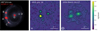 |
Fig. 1. Left: Hubble Space Telescope F814W (white) and ALMA Band 4 (red) imaging of RXJ1131−1231. Centre: ALMA imaging from 2015 July 19. Right: ALMA imaging from 2020 March 16 and 17. Contours start at ±2σ and increase by a factor of 2. The triplet images (A/B/C) and the AGN in the lensing galaxy (G) are clearly detected in ALMA data. We extract the mm-wave fluxes directly from the observed visibilities rather than the CLEANed images. |
2.2. ALMA observations and processing
The Atacama Large Millimeter/submillimeter Array (ALMA) first observed RXJ1131 at 2.1 mm (Band 4) on 2015 July 19 (ALMA project #2013.1.01207.S, PI: Paraficz; Paraficz et al. 2018). The data were taken using 37 12 m antennas, with baselines ranging between 28 m and 1.6 km. The full width at half maximum (FWHM) size of the synthesised beam was 0.39″ × 0.33″, with a surface brightness sensitivity σ = 11 μJy/beam (natural weighting); the maximum recoverable scale was 2.9″. The four spectral windows covered the frequency range of 136.1−140.0 and 148.0−152.0 GHz. The total on-source time was 1.3 h hours. Full details of observations are provided in Paraficz et al. (2018).
We re-observed RXJ1131 in 2.1 mm continuum on 2020 March 16 and 17 (ALMA Project #2019.1.00332.S, PI: Rybak) with the same spectral setup. To check if the source varies on ≈1-day timescales, the observations were taken in two blocks separated by 25 hours. The on-source time was 45.4 min per observation (90.8 min in total). The data were taken using 43 12 m antennas, with baselines ranging between 28 m and 943 m. The FWHM size of the synthesised beam was 0.85″ × 0.65″, with σ = 8 μJy/beam (natural weighting); the maximum recoverable scale was 9.1″.
All data were processed using the Common Astronomy Software Applications package (CASA; McMullin et al. 2007) version 4.7 for the 2015 data and 5.6 for the 2020 data. For the continuum imaging, we excluded a wide region around the CO(2−1) line (139−140 GHz). Finally, we created synthesised images with CASA’s tclean task, using natural weighting.
Figure 1 shows the synthesised ALMA imaging for 2015 July and 2020 March. At both epochs, four point-sources are visible: the triplet (A/B/C) and the AGN in the foreground galaxy (G). The lensed counterimage D is not significantly detected in either the 2015 or 2020 data. Table 1 lists the resulting beam size, sensitivity, and extracted fluxes.
Rest-frame 1.3 mm fluxes for the triplet images (A/B/C) and the foreground galaxy (G).
In addition to the four point-sources, the 2020 data show a faint, extended emission (peak surface brightness ≈20 μJy/beam), likely arising from the cold dust from extended star formation. After subtracting the point-sources (see below), the extended component accounts for S1.3 mm = 580 ± 60 μJy. The extended component is not detected in the 2015 data, which have significantly lower surface brightness sensitivities (42 μJy/arcsec2 in 2015 vs 7 μJy/arcsec2 in 2020) and a much smaller maximum recoverable scale (2.9″ in 2015 vs 9.1″ in 2020).
2.3. Visibility-plane analysis
We extracted the fluxes of the A/B/C triplet images and the foreground galaxy by directly fitting the observed visibilities3. Our free parameters are the x and y coordinates of the A image and the flux of the four point sources (A, B, C, and G; we did not use the D image). We fixed the spatial offsets between A, B, C, and G to the values predicted by the Suyu et al. lens model; changing the image separation to values from Paraficz et al. (2018) changes the inferred flux by ≤1%. We ran a Monte Carlo Markov chain using the emcee package (Foreman-Mackey et al. 2013). For the A-image position, we adopted a uniform prior with a 0.25″ diameter centred on the image position. Table 1 lists the inferred fluxes for individual datasets, with uncertainties inferred from uv-plane modelling.
Both the flux and flux ratios change significantly between the two epochs. In terms of flux, the A and B images have dimmed by a factor of 3.7 (≥60σ significance) and 2.3 (11σ) between 2015 and 2020, respectively. The C image flux derived from the uv-plane fit is consistent within 15% (1σ) between 2015 and 2020. The brightness of the AGN in the foreground galaxy (G) varied by 13% between 2015 and 2020 observations; this is likely a combination of intrinsic variability of the AGN (typical variability timescale ≤100 days, Baldi et al. 2015; Bower et al. 2015) and the ALMA Band 4 flux-calibration uncertainty (≈5% for each epoch).
In terms of flux ratios (Table 2), the A/B ratio decreases from 4.39 ± 0.12 to 2.72 ± 0.14 (7σ significance). The A/C ratio decreases from 13.99 ± 0.12 to 4.59 ± 0.44 (4.7σ). Finally, the C/B ratio increases from 0.32 ± 0.04 to 0.59 ± 0.08 (3.0σ).
1.3 mm rest-frame and optical flux ratios for individual epochs, compared to the macro lens model (Suyu et al. 2013) and mean values from the COSMOGRAIL 2004–2020 optical monitoring (Tewes et al. 2013; Millon et al. 2020).
Finally, we calculated the spectral index α (S ∝ να) by splitting the 2015 and 2020 data into the upper (150.1 GHz) and lower sideband (139.0 GHz). For the A image, we obtain α(2015) = 0.26 ± 0.4 and α(2015) = − 0.5 ± 0.3. For the B image, we obtain α(2015) = − 4 ± 2 and α(2020) = 1.0 ± 0.9. These values are consistent with a flat spectrum within 1−2σ.
2.4. Ancillary observations
RXJ1131 has extensive R-band monitoring spanning years 2003–2020 (Millon et al. 2020) from the COSMOGRAIL project (Courbin et al. 2005; Eigenbrod et al. 2005), primarily obtained using the Leonard Euler 1.2 m Swiss Telescope at La Silla, Chile. At the redshift of RXJ1131, the R-band corresponds to a rest-frame wavelength of 400 nm, which would trace the inner part of the accretion disc.
The closest optical data available in 2015 had been obtained on modified Julian date (MJD) 57 206 (16 days prior to ALMA observations). For the 2020 March data, we averaged the optical flux ratios obtained at MJD = 58 924.15 and 58 927.16, almost simultaneously with the ALMA data. The magnitudes of the lensed images are consistent between the two epochs within the uncertainties.
In addition to the ALMA observations presented above, RXJ1131 was observed with the Plateau de Bure Interferometer (PdBI) at 2.1 mm (matching the ALMA data) between 2014 December and 2015 February by Leung et al. (2017). The total flux of the triplet images at these epochs is just 0.39 ± 0.12 mJy in total, compared to 1.49 ± 0.1 mJy for ALMA 2015 July data. In other words, the total 2.1 mm flux brightened by a factor of ≈3 between 2015 February and July. Unfortunately, the low resolution of the PdBI data (beam FWHM 4.4″ × 2.0″) does not allow us to constrain the flux ratios for this epoch.
3. Results and analysis
Figure 2 compares the A/B, A/C, and C/B flux ratios observed with ALMA in 2015 and 2020 with the COSMOGRAIL R-band optical and Chandra X-ray monitoring. For the 2015 epoch, the ALMA and R-band flux ratios are noticeably different: namely, ALMA A/B and A/C ratios are significantly higher (at 8σ and 71σ significance, respectively) than optical ones. In 2020, the discrepancy between ALMA and R-band flux ratios is reduced to 3σ. The ALMA C/B flux ratio is lower than the optical one for the 2015 epoch, but consistent for the 2020 one.
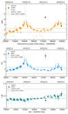 |
Fig. 2. Time evolution of the A/B, A/C, and C/B flux ratios as measured by ALMA, compared to the optical (COSMOGRAIL) and X-ray (Chandra) monitoring. We also show the average value of the R-band flux ratio (dashed line) and predicted value from the Suyu et al. (2013) lens model (dotted line). The amplitude of ALMA A/B flux ratio variations is comparable to that at optical and X-ray wavelengths but shifted in time, indicating different sizes or a spatial offset between the three components. |
Interestingly, the R-band monitoring (Fig. 2) shows a spectacularly high magnification of image A, peaking in 2009 June. The A/B and A/C optical ratios in 2009 were almost as extreme as the one measured in the 2015 ALMA data.
In strong gravitational lensing, the positions of point-like lensed images entirely determine their flux ratios. Large deviations between the observed and predicted flux ratios indicate either the presence of additional lensing mass (e.g. microlensing by stars, or massive dark-matter substructure) or that the source is time-variable. We considered the following three scenarios to explain the time-variable flux-ratio anomaly in RXJ1131: (i) microlensing of the mm-wave emission by stars in the lensing galaxy, (ii) a highly time-variable mm-wave source, and (iii) a change of magnification due to the relative proper motion of the source with respect to the foreground lens.
3.1. Microlensing analysis
We used microlensing modelling of the mm-wave and R-band (rest-frame UV) data to constrain the size of the mm-wave continuum emission. We put quantitative constraints on the mm-wave source size using a Bayesian framework to derive the probability distribution of the mm-wave source size by comparing the observed mm-wave flux ratios to microlensing simulations. We assumed that the mm-wave and optical emissionfollow circular Gaussian profiles and are co-centric.
For the optical flux ratios, we quadratically added a 0.2 mag systematic uncertainty reflecting the uncertainty on the level of regularisation of the AGN host galaxy when deconvolving the COSMOGRAIL monitoring data. We used the Tewes et al. (2013) photometry for the main analysis. Results obtained with the photometry of Millon et al. (2020) are presented in Appendix B.
For each lensed image, we calculated a microlensing magnification pattern using the inverse ray-shooting code of Wambsganss (1999, 2001). Each map was calculated accounting for the local value of convergence (κ) and shear (γ) from Sluse et al. (2012b).
The microlensing Einstein radius for RXJ1131 is
 (1)
(1)
where the D are angular diameter distances with the indices o, l, and s referring to observer, lens and source, respectively, and ⟨M⟩ is the average mass of the microlenses. For a mean stellar mass ⟨M⟩ = 0.3 M⊙, this corresponds to an Einstein radius of η0 = 0.008 pc.
We constructed square maps 20 η0 (0.16 pc) wide, with a resolution of 0.001 η0/pixel. Since the distance to the lens centre is approximately the same for all three quasar images, we set the surface density of stars along the line of sight to each image to be identical, κ⋆/κtot = 7%, representative of the stellar density at the Einstein radius (Schechter & Wambsganss 2004; Mediavilla et al. 2009; Pooley et al. 2012). We then drew 107 random positions in each map convolved with a Gaussian kernel corresponding to the half-light radius of the optical source size. For a given mm-wave observation, only realisations that match optical flux ratios within 3σ are kept, yielding a subset of ≈6 × 10⁶ positions. We then estimated the mm-wave flux ratios by varying the half-light radius of the mm-wave source from 0.0013 to 0.086 η0, in steps of 0.002 η0. For each of those positions, we calculated the A/B and A/C flux ratios and compared them to the data using chi-square statistic.
The distribution of inferred source sizes is shown in Fig. 3. While we cannot constrain the minimum size of the mm-wave emission with the current data, we obtain a 95th-percentile upper limit of R1/2 < 2.4 × 10⁻⁴ pc, equivalent to 50 AU. Given the estimated gravitational radius of Rg = GMBH/c2 = 5.7 × 10⁻⁶ pc (Sluse et al. 2012a; Chartas et al. 2017), this upper limit corresponds to R1/2 < 42 Rg. Relaxing the assumption of co-centricity increases the upper limit by a factor of ≈2, to R1/2 < 4.7 × 10⁻⁴ pc (82 Rg). The mm-wave source is too compact to be a dusty torus (which would be well within the dust sublimation radius) or the free-free emission from the broad-line region. Given the compactness of the mm-wave source at a few 10−4 pc, we attribute the mm-wave continuum to the AGN corona.
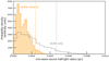 |
Fig. 3. Histogram of probability distributions of the half-light radius of the mm-wave emission, inferred from the microlensing analysis of ALMA and R-band data (orange) and ALMA data only (grey). |
In reality, the centroids of the mm-wave coronal emission and optical emission from the accretion disc could be spatially offset. Such offsets can be expect in, for example, the ‘lamp post’ model, where the peak of coronal emission is above the plane of accretion disc (Matt et al. 1991; Gonzalez et al. 2017; Marinucci et al. 2018).
While we cannot constrain the separation between the accretion disc and the mm-wave emission from two ALMA epochs, we can determine how the size of the mm-wave source depends on the co-spatiality assumption. Namely, we repeated our source size inference but ignoring the R-band data. The results are shown as the grey distribution in Fig. 3. The upper limit on the source size (95th percentile) increases to R1/2 < 4.7 × 10⁻⁴ pc = 82 Rg. This confirms that our results are not strongly affected by assuming that the R-band and mm-wave emission are co-centred.
3.2. Alternative scenarios for the mm-wave flux-ratio anomaly
3.2.1. Short-term variability of the background AGN
Studies of mm-wave variability in radio-quiet AGNs have found them to vary by a factor of a few over timescales of a few days (Michiyama et al. 2024; Shablovinskaya et al. 2024). In RXJ1131, the light from the source arrives first at image A, followed by images B and C. The high flux of the A image in 2015 could be explained by a ‘flare’ scenario: if the source brightness varies rapidly, the observations might have been taken just as the image A has brightened.
The time-delay between triplet images A and B is of the order of a few hours (Suyu et al. 2013). Consequently, for the flux-ratio anomaly to be caused by source variability, the source would have to brighten by a factor of ≈4 on a timescale of a few hours.
To check if mm-wave flux ratios vary on ≈1 day timescales, the 2020 observations were split into two blocks separated by ≈24 hours. The fluxes of individual images vary by A – 7%, B – 27%, and C – 12%, i.e. much less than required for explaining the 2015 flux-ratio anomaly. The triplet fluxes and flux ratios between the two 2020 blocks are consistent within 1.4σ.
We similarly looked for time variability in the 2015 data, which were taken in two blocks ≈1.5 h apart. The fluxes of individual images are consistent within 1σ between the two blocks. We therefore rule out intrinsic source variability as the source of the mm-wave flux-ratio anomaly in RXJ11314.
3.2.2. Relative lens–source motion
The high A/B flux ratio in 2015 might be explained by a presence of a massive dark-matter subhalo near the A image. However, a massive subhalo is hard to reconcile with the drastic change in A/B flux ratio over the five-year baseline. First, a static source-lens-subhalo constellation would produce flux-ratio anomalies that are constant in time – in clear disagreement with our observations. Second, the lack of a significant perturbation to the optical flux ratios already sets a strong upper limit on a subhalo radius of influence.
But could a scenario where the source and the lens/subhalo have a large relative proper motion be consistent with the change in A/B flux ratio? We examined the relative change in A/B flux ratio due to a proper motion of (1) a smooth lens and (2) a smooth lens and a subhalo, following Spingola et al. (2019). The relative proper motion between the lens and the source has to be slower than the speed of light c; consequently, the maximum lens-source displacement between 2015 and 2020 is Δμ ≤ c × 4.5 yr = 1.4 pc (in the lens plane), corresponding to an angular displacement of 0.32 mas.
We tested the impact of the lens-source displacement on the observed flux ratios by adopting the Suyu et al. (2013) lens model, a uniform-brightness circular source (R = 0.5 pc), and generating 1000 source–lens realisations with the lens randomly displaced by up to 0.32 mas assuming a uniform probability distribution. The triplet ratios vary by ≤5% even in this extreme scenario, too little to explain the observed change in flux ratios.
We then added a subhalo to the main lens. To maximise the flux-ratio perturbation caused by the subhalo, we assumed the subhalo to be centred on the A image for 2015 observations. We then applied a random displacement to the whole lens+subhalo system as described above. For the subhalo mass-density profile, we adopted a pseudo-Jaffe profile with a mass varying from Msub = 104 to 109 M⊙. The A/B flux ratio varies by ≤5% on average and ≤10% even in the most extreme cases: far too little to explain the observed flux-ratio fluctuations.
4. Discussion
4.1. Innermost structure of RXJ1131
How does our inferred mm-wave emission size compare to that of the accretion disc and the X-ray corona? Our upper limit is ≈2× larger than the size of the X-ray emission (R1/2, X = 26 Rg) and ≈3× smaller than the accretion disc, R1/2, UV = 147 Rg (Chartas et al. 2009; Dai et al. 2010). We sketch the relative sizes of the three components in Fig. 4. The mm-wave emission is significantly smaller than the accretion disc (traced by the UV) and comparable to the X-ray corona size.
 |
Fig. 4. Sketch of the relative sizes of mm-wave emission (orange), the X-ray corona (purple), and UV emission from the accretion disc (blue) in the centre of RXJ1131, derived from the microlensing analysis under the assumption that UV- and mm-wave emission are co-centric. The mm-wave emission is too compact to arise from a dusty torus; it is significantly smaller than the accretion disc and comparable to the X-ray corona size. 1 Rg = 5.7 × 10⁻⁶ pc. |
The different sizes of individual components are directly linked to their respective flux-ratio variabilities (Fig. 2): the X-ray variability is much higher than in optical wavelengths, indicating a more compact source. Curiously, the X-ray A/B flux ratio in the 2014–2016 epoch is a factor of a few smaller than the mm-wave one; simultaneous X-ray and mm-wave monitoring will be necessary to elucidate this behaviour.
4.2. Coronal emission: Millimetre-wave and X-ray luminosity
The inferred mm-wave luminosity (corrected for the lensing magnification) and size of RXJ1131 are consistent with the coronal scenario. In particular, the radio/mm-wave luminosity in radio-quiet quasars scales with X-ray luminosity (Laor & Behar 2008): at 100 GHz, Lmm ≈ 10−4LX (Behar et al. 2015, 2018; Ricci et al. 2023), similar to the phenomenological Güdel-Benz relation for coronally active cold stars, LR ≈ 10−4.5LX (Guedel & Benz 1993).
Figure 5 compares the mm-wave and X-ray luminosity (DeFrancesco et al. 2023) of RXJ1131 to a compilation of nearby AGNs (Behar et al. 2015, 2018; Ricci et al. 2023). With L100 GHz = LX × 10−4.3, RXJ1131 is remarkably close to the Güdel-Benz relation for stellar coronal emission. The size of the mm-wave emission in RXJ1131 is consistent with values inferred for low-redshift radio-quiet quasars using radiative transfer arguments: 10−4 to 10−3 pc (Behar et al. 2018; Shablovinskaya et al. 2024).
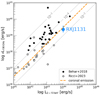 |
Fig. 5. Comparison of mm-wave and X-ray luminosities for RXJ1131 (blue) and local AGNs (Behar et al. 2018; Ricci et al. 2023). The mm-wave/X-ray luminosity ratio in RXJ1131 is consistent with predictions for coronal emission (L100 GHz/L2 − 10 keV = 10−4.5, orange line; Guedel & Benz 1993; Krucker & Benz 2000). |
The spectral slope measured between 139 and 150 GHz – α = −0.26 ± 0.4 matches expectations for the coronal emission from Raginski & Laor (2016), which predict a flat spectrum that will transition to a power law in the 300−1000 GHz regime.
4.3. Coronal magnetic field strength
Finally, we used the upper limit on the mm-wave corona size in RXJ1131 to estimate the magnetic field strength. Specifically, following Laor & Behar (2008), the size of an optically thick self-absorbed synchrotron source depends on its luminosity and the magnetic field B as
![Mathematical equation: $$ \begin{aligned} R\,\mathrm{[pc]} \approx 0.54 L_{39}^{1/2} \nu _{\rm GHz}^{-7/4} B_{\rm G}^{1/4}, \end{aligned} $$](/articles/aa/full_html/2025/09/aa54595-25/aa54595-25-eq2.gif) (2)
(2)
where R is the source size, L39 = νLν/(1039 erg/s), ν is the rest-frame frequency in GHz, and B is the magnetic field in Gauss.
We estimated B by inverting Eq. (2), using our upper limit on the mm-wave source size. To estimate νLν at 100 GHz, we adopted the 2020 flux measurements for the A/B/C triplet and assumed a flat spectral index. After correcting for the macro-model magnifications (i.e. neglecting any microlensing perturbations), we obtain a source-plane flux density of 6.5−15.6 μJy. The corresponding luminosity is νLν(230 GHz) = 3.0 − 7.1 × 1040 erg s−1. Consequently, the corresponding upper limits on the magnetic field strength are B ≤ 1.3 − 1.5 G (3σ). These upper limits are strikingly similar to the value of 1 G assumed by Behar et al. (2018) in their analysis of mm-wave emission in nearby AGNs, and somewhat lower then B = 5 − 18 G estimated by Shablovinskaya et al. (2024) for a nearby radio-quiet quasar IC 4329A. Note that according to Shablovinskaya et al. (2024), the coronal size in IC 4329A is a factor of a few larger than in RXJ 1131 (R ≈ 8 × 10⁻⁴ pc, ≈170 AU), which naturally implies a stronger magnetic field than in RXJ1131 (see Eq. (2)).
4.4. Spectral energy distribution of RXJ1131
As noted in Sect. 2, the integrated rest-frame 1.3 mm flux in RXJ1131 changes significantly between 2015 February (PdBI; Leung et al. 2017), 2015 July (ALMA), and 2020 March (ALMA). Figure 6 shows the ALMA and PdBI continuum measurements at 230 GHz, alongside photometry from Herschel (Stacey et al. 2018), LABOCA and PdBI (Leung et al. 2017), ALMA (Paraficz et al. 2018), and the Very Large Array (VLA; Becker et al. 1995; Wucknitz & Volino 2008). The 1.3 mm flux varies by a factor of ∼4 between 2015 February (Leung et al. 2017) and 2015 July (Paraficz et al. 2018).
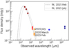 |
Fig. 6. SED of RXJ1131 over far-infrared to radio wavelengths, based on photometry from Herschel (dark red), LABOCA (red), and VLA (blue; see Stacey et al. 2018), and 1.3 mm fluxes (orange) from PdBI Leung et al. (2017) PdBI and ALMA (Paraficz et al. 2018, this work). Individual photometry points are summed up over all quasar images, and are not corrected for lensing magnification. The observed rest-frame 1.3 mm flux varies by a factor of ≈3 between different epochs. We show the best-fit modified-black body fits including the 2015 February (dashed) and 2015 July (dotted) PdBI and ALMA photometry; the inferred far-infrared luminosity and star-formation rates differ by a factor of ≈2. |
The time-variable emission from mm-wave corona is not included in most standard spectral energy distribution (SED) models (e.g. da Cunha et al. 2015; Calistro Rivera et al. 2016). Typically, in these SED models, the far-infrared to mm-wave emission is a composite of dust thermal emission (primarily from star formation, with a small contribution from the dusty torus in the AGN), and the free-free and synchrotron emission associated with star formation and a potential jet. Our results suggests that in some cases, time-variable coronal emission will dominate the emission at mm-wavelengths (as recently demonstrated for some nearby galaxies by del Palacio et al. 2025). This will have significant impact on the inferred galaxy properties, such as star-formation rates and dust masses.
As example, we fitted the available far-infrared and mm-wave photometry for RXJ1131 with a modified black-body SED, using ALMA fluxes from 2015 February (the faintest epoch) and 2015 July (the brightest), respectively. The inferred far-infrared luminosity in RXJ1131 varies between  and
and  , i.e. by a factor of ≈2. Assuming the Chabrier stellar initial mass function (Chabrier 2003), these estimates translate to star-formation rates of 290 ± 100 and 550 ± 150 M⊙/yr (without the lensing correction). In other words, the uncertainty due to the variable mm-wave emission is much higher than the nominal uncertainties from SED fitting.
The coronal contribution to the mm-wave flux might be particularly pronounced in lensed quasars, in which the compact quasar might be magnified by a higher factor than dust and gas in the galaxy (e.g. Serjeant 2012). Recent observations of mm-wave bright lensed quasars have already revealed significant variations on timescales of ≈10 years (Frias Castillo et al. 2024).
5. Conclusions
We report a significant time variability of mm-wave flux ratios in the quadruply lensed quasar RXJ 1131−1231. The flux ratios vary by a factor of a few between 2015 and 2020, but not on timescales of ≤1 day.
The changes in flux ratios are consistent with microlensing of a compact source with a half-light radius of ≤2.4 × 10⁻⁴ pc (50 AU). The inferred source size is robust with respect to the assumptions on the source geometry, stellar population of the lensing galaxy, and uncertainties on the lens model. Two alternative scenarios considered – a rapidly varying source and arelative proper motion between the lensing galaxy and the quasar – are not consistent with the data.
Given the compactness of the source, the most direct interpretation is that the mm-wave emission arises from the corona surrounding the central black hole. This is reinforced by the ratio of the mm-wave and X-ray luminosities, which follow the canonical Güdel-Benz relation for stellar coronae.
Our observations provide the first direct geometrical measurement of the size of the mm-wave AGN corona, which had previously been estimated using radiative transfer (Laor & Behar 2008; Shablovinskaya et al. 2024) or time-variability constraints (Baldi et al. 2015; Behar et al. 2020; Petrucci et al. 2023). These results highlight the promise of ALMA and NOEMA mm-wave monitoring to detect microlensing events in lensed quasars. Such future observations would be a powerful tool for studying the prevalence and detailed geometry of AGN coronae, and testing theoretical models for coronal emission.
While the mm VLBI with e.g. the Event Horizon Telescope, reaches resolutions down to ≈20 mas (Raymond et al. 2024), its limited sensitivity restricts it to just a handful of brightest sources in the mm-wave sky.
Throughout this paper, we assume a flat Λ cold dark matter cosmology, with Ωm = 0.315 and H0 = 67.4 km s−1 Mpc−1 (Planck Collaboration VI 2020). At redshift z = 0.658, 1″ corresponds to 7.187 kpc.
As a robustness check, we repeated the uv-plane procedure for the 2015 data, but taking only the baselines shorter than 968 m, i.e. as in the 2020 observations. The fluxes do not change appreciably.
Ultimately, a rapid time-variability would require the source to be very compact, with a size D ≃ c × 1 day = ≤10−3 pc, similar to the size inferred from the microlensing analysis.
Acknowledgments
M.R. is supported by the NWO Veni project “Under the lens” (VI.Veni.202.225). K.K.G. acknowledges the Belgian Federal Science Policy Office (BELSPO) for the provision of financial support in the framework of the PRODEX Programme of the European Space Agency (ESA). M.M. acknowledges support by the SNSF (Swiss National Science Foundation) through mobility grant P500PT_203114. E.B. was supported in part by a Center of Excellence of the Israel Science Foundation (grant No. 1937/19). F.C. acknowledges support from SNSF (Swiss National Science Foundation) in connection with observations with the Euler Swiss Telescope at ESO La Silla. This work is based on the research supported in part by the National Research Foundation of South Africa (Grant Number: 128943). This paper makes use of the following ALMA data: ADS/JAO.ALMA #2013.1.01207.S and #2019.1.00332.S. ALMA is a partnership of ESO (representing its member states), NSF (USA) and NINS (Japan), together with NRC (Canada), MOST and ASIAA (Taiwan), and KASI (Republic of Korea), in cooperation with the Republic of Chile. The Joint ALMA Observatory is operated by ESO, AUI/NRAO and NAOJ. This research has made use of data and software provided by the High Energy Astrophysics Science Archive Research Center (HEASARC), which is a service of the Astrophysics Science Division at NASA/GSFC and the High Energy Astrophysics Division of the Smithsonian Astrophysical Observatory. This research has made use of data obtained from the Chandra Data Archive and software provided by the Chandra X-ray Center (CXC) in the application packages CIAO and Sherpa. The authors are thankful for the assistance from Allegro, the European ALMA Regional Center node in the Netherlands. M.R. is especially thankful to J. Rybák for sparking interest in coronal emission.
References
- Baldi, R. D., Behar, E., Laor, A., & Horesh, A. 2015, MNRAS, 454, 4277 [Google Scholar]
- Baskin, A., & Laor, A. 2021, MNRAS, 508, 680 [NASA ADS] [CrossRef] [Google Scholar]
- Becker, R. H., White, R. L., & Helfand, D. J. 1995, ApJ, 450, 559 [Google Scholar]
- Behar, E., Baldi, R. D., Laor, A., et al. 2015, MNRAS, 451, 517 [NASA ADS] [CrossRef] [Google Scholar]
- Behar, E., Vogel, S., Baldi, R. D., Smith, K. L., & Mushotzky, R. F. 2018, MNRAS, 478, 399 [CrossRef] [Google Scholar]
- Behar, E., Kaspi, S., Paubert, G., et al. 2020, MNRAS, 491, 3523 [NASA ADS] [CrossRef] [Google Scholar]
- Bower, G. C., Markoff, S., Dexter, J., et al. 2015, ApJ, 802, 69 [Google Scholar]
- Calistro Rivera, G., Lusso, E., Hennawi, J. F., & Hogg, D. W. 2016, ApJ, 833, 98 [Google Scholar]
- Chabrier, G. 2003, PASP, 115, 763 [Google Scholar]
- Chartas, G., Kochanek, C. S., Dai, X., Poindexter, S., & Garmire, G. 2009, ApJ, 693, 174 [Google Scholar]
- Chartas, G., Krawczynski, H., Zalesky, L., et al. 2017, ApJ, 837, 26 [NASA ADS] [CrossRef] [Google Scholar]
- Chen, G. C. F., Suyu, S. H., Wong, K. C., et al. 2016, MNRAS, 462, 3457 [CrossRef] [Google Scholar]
- Courbin, F., Eigenbrod, A., Vuissoz, C., Meylan, G., & Magain, P. 2005, in Gravitational Lensing Impact on Cosmology, eds. Y. Mellier, & G. Meylan, 225, 297 [NASA ADS] [Google Scholar]
- da Cunha, E., Walter, F., Smail, I. R., et al. 2015, ApJ, 806, 110 [Google Scholar]
- Dai, X., Kochanek, C. S., Chartas, G., et al. 2010, ApJ, 709, 278 [Google Scholar]
- DeFrancesco, C. A., Dai, X., Mitchell, M., Zoghbi, A., & Morgan, C. W. 2023, ApJ, 959, 101 [Google Scholar]
- del Palacio, S., Yang, C., Aalto, S., et al. 2025, A&A, 701, A41 [NASA ADS] [CrossRef] [EDP Sciences] [Google Scholar]
- Di Matteo, T., Celotti, A., & Fabian, A. C. 1997, MNRAS, 291, 805 [Google Scholar]
- Doi, A., Kameno, S., Kohno, K., Nakanishi, K., & Inoue, M. 2005, MNRAS, 363, 692 [NASA ADS] [Google Scholar]
- Eigenbrod, A., Courbin, F., Vuissoz, C., et al. 2005, A&A, 436, 25 [NASA ADS] [CrossRef] [EDP Sciences] [Google Scholar]
- Falstad, N., Aalto, S., König, S., et al. 2021, A&A, 649, A105 [NASA ADS] [CrossRef] [EDP Sciences] [Google Scholar]
- Foreman-Mackey, D., Hogg, D. W., Lang, D., & Goodman, J. 2013, PASP, 125, 306 [Google Scholar]
- Frias Castillo, M., Rybak, M., Hodge, J., et al. 2024, A&A, 683, A211 [NASA ADS] [CrossRef] [EDP Sciences] [Google Scholar]
- Gonzalez, A. G., Wilkins, D. R., & Gallo, L. C. 2017, MNRAS, 472, 1932 [Google Scholar]
- Guedel, M., & Benz, A. O. 1993, ApJ, 405, L63 [NASA ADS] [CrossRef] [Google Scholar]
- Inoue, Y., & Doi, A. 2018, ApJ, 869, 114 [Google Scholar]
- Jiménez-Vicente, J., Mediavilla, E., Kochanek, C. S., & Muñoz, J. A. 2015, ApJ, 799, 149 [Google Scholar]
- Krucker, S., & Benz, A. O. 2000, Sol. Phys., 191, 341 [Google Scholar]
- Laor, A., & Behar, E. 2008, MNRAS, 390, 847 [NASA ADS] [CrossRef] [Google Scholar]
- Leung, T. K. D., Riechers, D. A., & Pavesi, R. 2017, ApJ, 836, 180 [Google Scholar]
- Marinucci, A., Tamborra, F., Bianchi, S., et al. 2018, Galaxies, 6, 44 [Google Scholar]
- Matt, G., Perola, G. C., & Piro, L. 1991, A&A, 247, 25 [NASA ADS] [Google Scholar]
- McMullin, J. P., Waters, B., Schiebel, D., Young, W., & Golap, K. 2007, ASP Conf. Ser., 376, 127 [Google Scholar]
- Mediavilla, E., Munoz, J. A., Falco, E., et al. 2009, ApJ, 706, 1451 [NASA ADS] [CrossRef] [Google Scholar]
- Michiyama, T., Inoue, Y., Doi, A., et al. 2024, ApJ, 965, 68 [NASA ADS] [CrossRef] [Google Scholar]
- Millon, M., Courbin, F., Bonvin, V., et al. 2020, A&A, 640, A105 [NASA ADS] [CrossRef] [EDP Sciences] [Google Scholar]
- Panessa, F., Baldi, R. D., Laor, A., et al. 2019, Nat. Astron., 3, 387 [Google Scholar]
- Paraficz, D., Rybak, M., McKean, J. P., et al. 2018, A&A, 613, A34 [NASA ADS] [CrossRef] [EDP Sciences] [Google Scholar]
- Petrucci, P. O., Piétu, V., Behar, E., et al. 2023, A&A, 678, L4 [NASA ADS] [CrossRef] [EDP Sciences] [Google Scholar]
- Planck Collaboration VI. 2020, A&A, 641, A6 [NASA ADS] [CrossRef] [EDP Sciences] [Google Scholar]
- Pooley, D., Rappaport, S., Blackburne, J. A., Schechter, P. L., & Wambsganss, J. 2012, ApJ, 744, 111 [NASA ADS] [CrossRef] [Google Scholar]
- Raginski, I., & Laor, A. 2016, MNRAS, 459, 2082 [CrossRef] [Google Scholar]
- Raymond, A. W., Doeleman, S. S., Asada, K., et al. 2024, AJ, 168, 130 [NASA ADS] [CrossRef] [Google Scholar]
- Reis, R. C., Reynolds, M. T., Miller, J. M., & Walton, D. J. 2014, Nature, 507, 207 [NASA ADS] [CrossRef] [Google Scholar]
- Ricci, C., Chang, C.-S., Kawamuro, T., et al. 2023, ApJ, 952, L28 [NASA ADS] [CrossRef] [Google Scholar]
- Schechter, P. L., & Wambsganss, J. 2004, in Dark Matter in Galaxies, eds. S. Ryder, D. Pisano, M. Walker, & K. Freeman, 220, 103 [NASA ADS] [Google Scholar]
- Serjeant, S. 2012, MNRAS, 424, 2429 [NASA ADS] [CrossRef] [Google Scholar]
- Shablovinskaya, E., Ricci, C., Chang, C. S., et al. 2024, A&A, 690, A232 [NASA ADS] [CrossRef] [EDP Sciences] [Google Scholar]
- Sluse, D., Surdej, J., Claeskens, J. F., et al. 2003, A&A, 406, L43 [NASA ADS] [CrossRef] [EDP Sciences] [Google Scholar]
- Sluse, D., Hutsemékers, D., Lamy, H., Cabanac, R., & Quintana, H. 2005, A&A, 433, 757 [NASA ADS] [CrossRef] [EDP Sciences] [Google Scholar]
- Sluse, D., Claeskens, J. F., Hutsemékers, D., & Surdej, J. 2007, A&A, 468, 885 [NASA ADS] [CrossRef] [EDP Sciences] [Google Scholar]
- Sluse, D., Hutsemékers, D., Courbin, F., Meylan, G., & Wambsganss, J. 2012a, A&A, 544, A62 [NASA ADS] [CrossRef] [EDP Sciences] [Google Scholar]
- Sluse, D., Chantry, V., Magain, P., Courbin, F., & Meylan, G. 2012b, A&A, 538, A99 [NASA ADS] [CrossRef] [EDP Sciences] [Google Scholar]
- Spingola, C., McKean, J. P., Massari, D., & Koopmans, L. V. E. 2019, A&A, 630, A108 [NASA ADS] [CrossRef] [EDP Sciences] [Google Scholar]
- Stacey, H. R., McKean, J. P., Robertson, N. C., et al. 2018, MNRAS, 476, 5075 [NASA ADS] [CrossRef] [Google Scholar]
- Suyu, S. H., Auger, M. W., Hilbert, S., et al. 2013, ApJ, 766, 70 [Google Scholar]
- Tewes, M., Courbin, F., & Meylan, G. 2013, A&A, 553, A120 [NASA ADS] [CrossRef] [EDP Sciences] [Google Scholar]
- Wambsganss, J. 1999, J. Comput. Appl. Math., 109, 353 [NASA ADS] [CrossRef] [Google Scholar]
- Wambsganss, J. 2001, PASA, 18, 207 [Google Scholar]
- Wucknitz, O., & Volino, F. 2008, ArXiv e-prints [arXiv:0811.3421] [Google Scholar]
Appendix A: Visibility-plane models
Figure A.1 shows the dirty images of the 2015 and 2020 data, best-fitting models, and dirty-image residuals. Looking at the residuals, it is clear that the four-point-source model does not provide a perfect fit to the data. First, as already seen in Fig. 1, the 2020 data reveal a faint, extended dust emission. This extended emission peaks in the vicinity of the D image, indicating a potential leftover continuum signal from the AGN.
In addition, the 2015 data show significant (∼5σ) residuals around the A-image: potentially dust emission from a circumnuclear star-forming region. We attempted to include the extended emission around the A-image in our uv-plane modelling as a circular Gaussian component centred on the A-image; this reduces the flux of the point-source component of image A by ∼15%, but does not significantly improve the quality of the fit. The inferred flux ratios are thus largely unaffected by the extended emission.
We note that subtracting an extended component (scaled for the relative magnification factors from Table 1) from the A/B/C images would make the resulting flux ratios for a point-like component even more extreme – thus strengthening the case for the microlensing scenario.
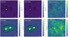 |
Fig. A.1. Results of the uv-fitting procedure. The individual columns show dirty images of the data, model, and the residuals (data minus model). The 2015 and 2020 observations are shown in the upper and lower row, respectively. The contours are drawn at ±(2, 3, 4, …)σ levels. After fitting the four point-sources, the 2015 data show significant (∼5σ) residuals around the A-image, likely dust in the circumnuclear region. For the 2020 data, residuals show the faint, extended emission from the cold dust in the gaseous disc. |
Appendix B: Microlensing analysis: Systematic tests
In this section we present the results of the mm-wave source size inference when (a) using the photometric light curve published by Millon et al. (2020) instead of the one of Tewes et al. (2013); and (b) assuming a higher value of the stellar fraction at the Einstein radius, specifically κ⋆/κtot = 0.3 instead of 0.07. The first systematic test is motivated by the systematic decrease of about 0.27 mag in the magnitude of image A between deconvolved photometry in Tewes et al. (2013) and Millon et al. (2020). Adopting the values from latter, we find R1/2 < 3.2 × 10⁻⁴ pc, an increase of about 25% of the upper bound on the mm-wave source size.
The second test evaluates the impact of our choice of κ⋆/κtot on the results. By analysing the rest-frame UV flux ratios of a large sample lensed quasars (but excluding RXJ1131 due to its lower redshift), Jiménez-Vicente et al. (2015) simultaneously derived the stellar mass fraction and UV source size. They found that κ⋆/κtot = 0.2 ± 0.1 was favoured by the data. We repeated our calculation by fixing κ⋆/κtot = 0.3, i.e. the higher end of the Jiménez-Vicente et al. (2015) estimate. In that case, we derive R1/2 < 1.4 × 10⁻⁴ pc when using the photometry of Tewes et al. (2013), and R1/2 < 2.5 × 10⁻⁴ pc using that of Millon et al. (2020). This is about 25% smaller than the value obtained in our main analysis. Table B.1 summarises these results.
These tests show that the systematic uncertainty on the mm-wave source size should be of the order of 0.2 dex due to the systematic uncertainties on the photometry and on the uncertainty on the fraction of compact objects towards the lensed images. Such systematic uncertainties have no discernable impact on our conclusions.
Comparison of upper limits on the source size derived using different assumptions on κ⋆ and photometry measurements.
All Tables
Rest-frame 1.3 mm fluxes for the triplet images (A/B/C) and the foreground galaxy (G).
1.3 mm rest-frame and optical flux ratios for individual epochs, compared to the macro lens model (Suyu et al. 2013) and mean values from the COSMOGRAIL 2004–2020 optical monitoring (Tewes et al. 2013; Millon et al. 2020).
Comparison of upper limits on the source size derived using different assumptions on κ⋆ and photometry measurements.
All Figures
|
Fig. 1. Left: Hubble Space Telescope F814W (white) and ALMA Band 4 (red) imaging of RXJ1131−1231. Centre: ALMA imaging from 2015 July 19. Right: ALMA imaging from 2020 March 16 and 17. Contours start at ±2σ and increase by a factor of 2. The triplet images (A/B/C) and the AGN in the lensing galaxy (G) are clearly detected in ALMA data. We extract the mm-wave fluxes directly from the observed visibilities rather than the CLEANed images. |
| In the text | |
|
Fig. 2. Time evolution of the A/B, A/C, and C/B flux ratios as measured by ALMA, compared to the optical (COSMOGRAIL) and X-ray (Chandra) monitoring. We also show the average value of the R-band flux ratio (dashed line) and predicted value from the Suyu et al. (2013) lens model (dotted line). The amplitude of ALMA A/B flux ratio variations is comparable to that at optical and X-ray wavelengths but shifted in time, indicating different sizes or a spatial offset between the three components. |
| In the text | |
|
Fig. 3. Histogram of probability distributions of the half-light radius of the mm-wave emission, inferred from the microlensing analysis of ALMA and R-band data (orange) and ALMA data only (grey). |
| In the text | |
|
Fig. 4. Sketch of the relative sizes of mm-wave emission (orange), the X-ray corona (purple), and UV emission from the accretion disc (blue) in the centre of RXJ1131, derived from the microlensing analysis under the assumption that UV- and mm-wave emission are co-centric. The mm-wave emission is too compact to arise from a dusty torus; it is significantly smaller than the accretion disc and comparable to the X-ray corona size. 1 Rg = 5.7 × 10⁻⁶ pc. |
| In the text | |
|
Fig. 5. Comparison of mm-wave and X-ray luminosities for RXJ1131 (blue) and local AGNs (Behar et al. 2018; Ricci et al. 2023). The mm-wave/X-ray luminosity ratio in RXJ1131 is consistent with predictions for coronal emission (L100 GHz/L2 − 10 keV = 10−4.5, orange line; Guedel & Benz 1993; Krucker & Benz 2000). |
| In the text | |
|
Fig. 6. SED of RXJ1131 over far-infrared to radio wavelengths, based on photometry from Herschel (dark red), LABOCA (red), and VLA (blue; see Stacey et al. 2018), and 1.3 mm fluxes (orange) from PdBI Leung et al. (2017) PdBI and ALMA (Paraficz et al. 2018, this work). Individual photometry points are summed up over all quasar images, and are not corrected for lensing magnification. The observed rest-frame 1.3 mm flux varies by a factor of ≈3 between different epochs. We show the best-fit modified-black body fits including the 2015 February (dashed) and 2015 July (dotted) PdBI and ALMA photometry; the inferred far-infrared luminosity and star-formation rates differ by a factor of ≈2. |
| In the text | |
|
Fig. A.1. Results of the uv-fitting procedure. The individual columns show dirty images of the data, model, and the residuals (data minus model). The 2015 and 2020 observations are shown in the upper and lower row, respectively. The contours are drawn at ±(2, 3, 4, …)σ levels. After fitting the four point-sources, the 2015 data show significant (∼5σ) residuals around the A-image, likely dust in the circumnuclear region. For the 2020 data, residuals show the faint, extended emission from the cold dust in the gaseous disc. |
| In the text | |
Current usage metrics show cumulative count of Article Views (full-text article views including HTML views, PDF and ePub downloads, according to the available data) and Abstracts Views on Vision4Press platform.
Data correspond to usage on the plateform after 2015. The current usage metrics is available 48-96 hours after online publication and is updated daily on week days.
Initial download of the metrics may take a while.