| Issue |
A&A
Volume 701, September 2025
|
|
|---|---|---|
| Article Number | A133 | |
| Number of page(s) | 29 | |
| Section | Planets, planetary systems, and small bodies | |
| DOI | https://doi.org/10.1051/0004-6361/202554885 | |
| Published online | 12 September 2025 | |
Reliability of 1D radiative-convective photochemical-equilibrium retrievals on transit spectra of WASP-107b
1
Institute of Astronomy, KU Leuven,
Celestijnenlaan 200D,
3001
Leuven,
Belgium
2
Centre for Exoplanet Science, University of Edinburgh,
Edinburgh
EH9 3FD,
UK
3
School of GeoSciences, University of Edinburgh,
Edinburgh,
EH9 3FF,
UK
4
Anton Pannekoek Institute for Astronomy, University of Amsterdam,
Science Park 904,
1098
XH
Amsterdam,
The Netherlands
5
Royal Observatory of Belgium,
Ringlaan 3,
1180
Brussels,
Belgium
6
University of Liège, STAR Institute,
Allée du Six Août 19C,
4000
Liège,
Belgium
★ Corresponding author.
Received:
31
March
2025
Accepted:
13
July
2025
Abstract
Context. WASP-107b has been observed in unprecedented detail with the James Webb Space Telescope. These observations suggest that it has a metal-rich and carbon-deprived atmosphere with an extremely hot interior based on detections of SO2, H2O, CO2, CO, NH3, and CH4.
Aims. In this paper, we aim to determine the reliability of a 1D radiative-convective photochemical-equilibrium (1D-RCPE) retrieval method in inferring atmospheric properties of WASP-107b. We aim to explore its sensitivity to modelling assumptions and different cloud parametrizations, and investigate the data information content. Additionally, we aim to characterize chemical trends and map dominant pathways to develop a comprehensive understanding of the 1D-RCPE model grid before running the retrievals.
Methods. We built a grid of radiative-convective balanced pressure-temperature profiles and 1D photochemical equilibrated models, which cover a range of metallicities (Z), carbon-to-oxygen ratios (C/O), intrinsic temperatures (Tint), and eddy diffusion coefficients (Kzz). We adopted a nested sampling algorithm within a Bayesian framework to estimate model parameters from previously analysed transit observations of WASP-107b discontinuously covering 1.1–12.2 μm.
Results. Our model grid reproduces established chemical trends such as the dependence of SO2 production on metallicity and demonstrates that mixing-induced quenching at high Tint reduces the bulk CH4 and NH3 content. We obtain good fits with our 1D-RCPE retrievals that are mostly based on a few molecular features of H2O, CO2, SO2, and CH4, but find no substantial contribution of NH3. We find that the degeneracy between metallicity, cloud pressure, and a model offset is broken by the presence of strong SO2 features, confirming that SO2 is a robust metallicity indicator. We systematically retrieve sub-solar C/O based on the relative amplitude of a strong CO2 feature with respect to the broad band of H2O, which is sensitive to a wavelength-dependent scattering slope. We find that high-altitude clouds obscure the CH4−rich layers, preventing the retrievals from constraining Tint, but that higher values of Kzz can transport material above the cloud deck, allowing a fit of the CH4 feature. However, Tint and Kzz can vary substantially between retrievals depending on the adopted cloud parametrization.
Conclusions. We conclude that the 1D-RCPE retrieval method can provide useful insights if the underlying grid of forward models is well understood. We find that WASP-107b’s atmosphere is enriched in metals (3–5 Z⊙) and carbon-deprived (C/O ≲ 0.20). However, we lack robust constraints on the intrinsic temperature and vertical mixing strength.
Key words: astrochemistry / planets and satellites: atmospheres / planets and satellites: composition
© The Authors 2025
 Open Access article, published by EDP Sciences, under the terms of the Creative Commons Attribution License (https://creativecommons.org/licenses/by/4.0), which permits unrestricted use, distribution, and reproduction in any medium, provided the original work is properly cited.
This article is published in open access under the Subscribe to Open model. This email address is being protected from spambots. You need JavaScript enabled to view it. to support open access publication.
1 Introduction
WASP-107b is a transiting exoplanet orbiting a K7V-type host star at a distance of 0.055 AU, resulting in an equilibrium temperature of ∼740 K (Anderson et al. 2017). With a mass of 0.12 MJup and a radius of 0.90 RJup (Piaulet et al. 2021), its extremely low gravity and large scale height make it well suited for atmospheric characterization. A series of transit observations have revealed the structure of WASP-107b’s deeper atmosphere in unprecedented detail. Observations with the Hubble Space Telescope (HST) in the near-infrared show water vapour features, compressed by high-altitude clouds (Kreidberg et al. 2018). Further observations with James Webb Space Telescope’s (JWST) MIRI instrument (LRS) were obtained by Dyrek et al. (2024), who further constrained the type of aerosols to silicate cloud particles (i.e. MgSiO3, SiO2, and SiO). Additionally, the detection of SO2 is indicative of photochemistry in a metal-enriched atmosphere (Tsai et al. 2023; Dyrek et al. 2024).
Neither dataset shows proof of CH4, despite predictions from equilibrium chemistry showing that methane should be abundant at temperatures below ∼1000 K (Moses et al. 2011). Vertical mixing drives the atmosphere out of equilibrium and can quench CH4 in the deep atmosphere, thereby fixing the methane content in higher layers to the volume mixing ratio (VMR) at the quench point. In addition to possible carbon depletion by a sub-solar carbon-to-oxygen ratio, Dyrek et al. (2024) show that the combination of a high intrinsic temperature and strong vertical mixing reduces the CH4 content to undetectable levels without affecting the formation of SO2 in the upper layers (see their Extended Data – Figure 3).
More recently, Welbanks et al. (2024) analysed JWST NIRCam spectra in combination with previous datasets and managed to detect and constrain the abundances of H2O, SO2, CO, CO2, NH3, and even traces of CH4. These results were accompanied by the publication of Sing et al. (2024), who used a JWST NIRSpec spectrum to detect H2O, SO2, CO, CO2, and CH4. Both of the above studies conclude that the depleted CH4 is the result of a high intrinsic temperature (>350 K) and atmospheric mixing causing deep quenching. Additionally, Welbanks et al. (2024) attribute this hot interior to eccentricity-driven tidal heating, which had previously been identified as a potential explanation for the inflated radius of WASP-107b (Thorngren et al. 2019; Fortney et al. 2020; Yu & Dai 2024).
Atmospheric retrievals aim to infer basic properties from observations by navigating a large, degenerate parameter space using parametrized, easy-to-compute models and Bayesian inference techniques (Madhusudhan 2018). However, such simplifications can lead to biases for inferred parameters, which have been documented and investigated in the past (e.g. Benneke & Seager 2012; Griffith 2014; Line & Parmentier 2016; Heng & Kitzmann 2017; Fisher & Heng 2018; Welbanks & Madhusudhan 2019; MacDonald et al. 2020; Novais et al. 2025). Alternatively, one can construct more complex forward models that take into account, for example, chemical kinetics (e.g. in Dyrek et al. 2024), radiative-convective equilibrium, cloud microphysics, and fluid dynamics. A major downside of forward models is the large computational cost, which makes them unsuited for retrievals. Combining the best of both worlds, Bell et al. (2023) introduced a 1D radiative-convective photochemicalequilibrium (1D-RCPE) retrieval (Beatty et al. 2024; Fu et al. 2024; Welbanks et al. 2024). By pre-computing a grid of physics-informed forward models, and allowing for interpolation in between, 1D-RCPE retrievals can leverage the strength of Bayesian inference with on-the-fly computation of low-cost forward models. This technique was applied to WASP-107b by Welbanks et al. (2024), who deduced a high intrinsic temperature based on the CH4 deficiency.
Given WASP-107b’s inflated radius and low density, the atmospheric elemental composition and intrinsic temperature can help to unravel properties such as the planet’s core mass, and formation history (Madhusudhan et al. 2016; Anderson et al. 2017; Piaulet et al. 2021; Welbanks et al. 2024; Sing et al. 2024). To achieve this, it is crucial to deduce the atmospheric properties from transit spectra as accurately as possible. Various methods have been adopted in the above studies, which lead to different results. More specifically for WASP-107b, reported values for atmospheric metallicity range from ≳ 6 Z⊙ (Dyrek et al. 2024) up to 43 ± 8 Z⊙ (Sing et al. 2024), and for carbon-to-oxygen ratios from  (solar) (Sing et al. 2024) down to
  (Welbanks et al. 2024). Additionally, multiple studies on WASP107b point towards a high intrinsic temperature and deep quenching based on the lack of strong CH4 features.
In this paper, we aim to assess how well 1D-RCPE retrievals can reliably infer atmospheric properties such as metallicity (Z), carbon-to-oxygen ratio (C/O), intrinsic temperature (Tint), and eddy diffusion coefficient (Kzz) for WASP-107b. More specifically, we explore the sensitivity of our results to different cloud parametrizations, and investigate the information content of the available observations. A secondary goal of this paper is to consistently analyse the relevant chemical pathways and summarize the chemical trends with respect to the four grid parameters (Z, C/O, Tint, and Kzz).
In Sect. 2, we describe the methods and numerical codes used in this study. We start by constructing a grid of 900 1D-RCPE models and analyse the results in Sect. 3. We then proceed by running 1D-RCPE retrievals with various set-ups in Sect. 4. Finally, in Sect. 5, we discuss how our results affect previously inferred properties of WASP-107b before concluding in Sect. 6.
2 Methods
We used a number of different codes to build and analyse our grid of 1D-RCPE models. First, we outline the design of our model grid (Sect. 2.1). This is followed by description of our model set-up for the pressure-temperature profiles with PICASO (Sect. 2.2) and the chemical kinetics simulations with VULCAN (Sect. 2.3). We analysed the resulting grid of 900 1D-RCPE models with Dijkstra’s algorithm (Sect. 2.4). To generate synthetic transit spectra, we used petitRADTRANS (Sect. 2.5) with various cloud parametrizations (Sect. 2.6). Finally, we fitted the 1D-RCPE model grid to different datasets (Sect. 2.7) with UltraNest (Sect. 2.8).
2.1 Grid design
We varied four parameters in our grid of forward models: Z, C/O, Tint, and Kzz. We ran atmospheric models with metallicities 1, 2, 3, 5, 7, 10, 15, 20, and 30 Z⊙ (Asplund et al. 2009). We discarded sub-solar values based on previous findings and the detection of SO2, which points to metal enrichment (Kreidberg et al. 2018; Dyrek et al. 2024). The upper limit was chosen based on the interior structure models that estimate the planet’s maximal bulk metallicity (Kreidberg et al. 2018; Thorngren & Fortney 2019). We explored C/O ratios of 0.05, 0.11, 0.23, and 0.46, corresponding to roughly 10%, 25%, 50%, and 100% of the solar value, respectively (Lodders 2010), in agreement the lower boundary suggested by planet formation models (Öberg et al. 2011; Mordasini et al. 2016; Espinoza et al. 2017). We considered intrinsic temperatures of 100, 200, 300, 400, and 500 K. The lower values correspond to the predictions where only deposition of stellar radiation is considered (Thorngren et al. 2019), while higher values correspond to increasing effects of tidal heating (Leconte et al. 2010; Fortney et al. 2020; Millholland et al. 2020). We explored eddy diffusion coefficients of 106, 107, 108, 109, and 1010 cm2/s, corresponding to atmospheres with and without quenching. Combined, this results in a grid of 900 forward models. Throughout the grid, we used parameters that are representative for the WASP-107(b) system. For WASP-107b, these include a surface gravity of 270 cm/s2, radius of 0.94 RJup, mass of 0.10 MJup, orbital separation of 0.055 AU, and equilibrium temperature of 740 K. For its host star, we adopted  , a radius of 0.66 R⊙, and log g(cgs) ≃ 4.6 (Piaulet et al. 2021).
2.2 Radiative-convective equilibrium: PICASO
We used the open-source 1D radiative-convective code PICASO (Mukherjee et al. 2023) to compute 180 temperature-pressure profiles of the atmosphere of WASP-107b, each with a different metallicity, carbon-to-oxygen ratio, and intrinsic temperature. We ran PICASO with 91 pressure log-spaced levels between 300 and 10−7 bar. The code uses pre-mixed correlated-k opacities that are calculated under the assumption of equilibrium chemistry (Lupu et al. 2023; Mukherjee et al. 2023). As is listed in Lupu et al. (2023), these include C2H2 (Wilzewski et al. 2016; Rothman et al. 2013), C2H4 (Rothman et al. 2013; Marley et al. 2021), C2H6 (Rothman et al. 2013; Marley et al. 2021), CH4 (Yurchenko et al. 2013; Yurchenko & Tennyson 2014; Pine 1992; Wenger & Champion 1998), CO (Rothman et al. 2010; Gordon et al. 2017; Li et al. 2015), CO2 (Huang et al. 2014), CrH (Burrows et al. 2002), Fe (Ryabchikova et al. 2015; O’Brian et al. 1991; Fuhr et al. 1988; Bard et al. 1991; Bard & Kock 1994), FeH (Dulick et al. 2003; Hargreaves et al. 2010), H2 (Gordon et al. 2017),  (Mizus et al. 2017), H2O Polyansky et al. (2018); Barton et al. (2017), H2S (Azzam et al. 2016; Rothman et al. 2013; Marley et al. 2021), HCN (Harris et al. 2006; Barber et al. 2014; Gordon et al. 2022), LiCl (Bittner & Bernath 2018), LiF (Bittner & Bernath 2018), LiH (Coppola et al. 2011), MgH (GharibNezhad et al. 2013; Yadin et al. 2012; Gharib-Nezhad et al. 2021), N2 (Rothman et al. 2013; Marley et al. 2021), NH3 (Yurchenko et al. 2011; Wilzewski et al. 2016; Marley et al. 2021), OCS (Gordon et al. 2017), PH3 (Sousa-Silva et al. 2014; Marley et al. 2021), SiO (Barton et al. 2013; Kurucz 1992; Marley et al. 2021), TiO (McKemmish et al. 2019; Gharib-Nezhad et al. 2021), and VO (McKemmish et al. 2019; Gharib-Nezhad et al. 2021; Marley et al. 2021), in addition to alkali metals (Li, Na, K, Rb, Cs) (Ryabchikova et al. 2015; Allard et al. 2019, 2016, 2007a, b). For a planet such as WASP107b, H2O and potentially CH4 are expected to be the dominant infrared absorbers (Mollière et al. 2015).
In order to converge to a solution with a smooth transition between the radiative and convective layers, PICASO requires an initial guess of the pressure level of the radiative-convective boundary zone (RCB). As the RCB is highly sensitive to Tint (Sarkis et al. 2021), we varied the RCB pressure level for each model with different intrinsic temperatures to ensure said convergence. The pre-computed opacity mixtures in PICASO do not include metallicities 7 and 15 Z⊙. Therefore, we linearly interpolated these PT structures from neighbouring metallicities (5 to 10 Z⊙, and 10 to 20 Z⊙, respectively). For models with C/O=0.05, we used the same computation as C/O=0.11 as such low carbon-to-oxygen ratios are not available in the opacity data. Finally, we chose to compute day-side averages by setting rst=1, which controls the contribution of stellar radiation to the net radiative flux in every atmospheric layer (see Eq. (20) in Mukherjee et al. 2023), so that the temperature in the upper, quasi-isothermal layers matches the reported values in Dyrek et al. (2024). We further discuss this assumption in Sect. 5. Fig. 1 shows a selection of the computed PT profiles with PICASO.
2.3 (Photo)-chemical modelling: VULCAN
We used the open-source chemical kinetics code VULCAN (Tsai et al. 2017, 2021) to model the molecular composition of WASP-107b. We used the default chemical network SNCHO_PHOTO_NETWORK that includes 89 species composed of H, C, O, N, S, coupled by 1030 forward and backward thermochemical reactions. Vertical mixing was included via diffusion, with accompanying eddy diffusion coefficient Kzz. We used a constant Kzz profile for each model, with the values specified in Sect. 2.1, to reduce complexity and maintain good interpretability of our results.
Photochemistry was included by way of 60 photodissociation reactions for the main UV absorbing species in H2−dominated atmospheres. We used a spectral energy distribution (SED) of HD 85512, as a proxy for host star WASP-107. HD 85512 is a K7V star with a similar effective temperature as WASP-107, and its SED is available in the MUSCLES database (France et al. 2016; Youngblood et al. 2016; Loyd et al. 2016). Note that the SEDs of stars with similar spectral types are not necessarily comparable, as high-energy (X-ray, UV) radiation fluxes are linked to stellar age, rotation period and overall magnetic activity, rather than photospheric emission. With a rotation period of 17 ± 1 days (Anderson et al. 2017) and age of 3.4 ± 0.7 Gyr (Piaulet et al. 2021), WASP-107 is expected to be more active compared to HD 85512, which has a ∼47 day rotation period and a resulting age estimate of 5.6 ± 0.1 Gyr (Tsantaki et al. 2013). However, observations in the NUV and X-ray have shown that WASP-107 is slightly less active than HD 85512, although this difference is less than a factor of two in the UV so that HD 85512 remains a good proxy for WASP-107 (Dyrek et al. 2024).
To initialise VULCAN, we used 150 log-spaced vertical layers between 10 and 10−7 bar for models with high Tint to ensure convergence in the deep layers, while this upper pressure boundary can be extended to 300 bar for low Tint to capture the quenching points. To fix individual convergence issues, we lowered parameters ATOL and/or RTOL (absolute and relative tolerance thresholds for errors during the numerical integration), or systematically decreased the pressure boundary at the interior while making sure the quench points of key species (i.e. CH4 and NH3) are captured in the model. Otherwise, we used the default set-up of VULCAN. The above adjustments were especially necessary for models with low Kzz, where the quench points are located much higher than their high- Kzz counterparts.
The elemental mixture was adjusted based on the given combination of Z and C/O, before the simulation is started from chemical equilibrium abundances. We first scaled the solar elemental mixture (Asplund et al. 2009) with the Z, before lowering the carbon abundance to the requested C/O. We did not include processes such as condensation, ion chemistry, or atmospheric escape. Finally, we highlight that VULCAN assumes a fixed thermal background during the numerical integration. Studies have shown that the introduction of disequilibrium chemistry can lead to temperature differences up to 100 K in the PT profile (Drummond et al. 2016; Agúndez 2025).
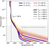 |
Fig. 1 Selection of the 180 computed PT profiles with PICASO for C/O=0.46. The line transparency corresponds to intrinsic temperature, from a full line for Tint=100 K to almost transparent for Tint=500 K. The shaded grey region indicates layers where the radiative-convective boundaries are located in all 180 PT profiles. |
2.4 Chemical pathway analysis: Dijkstra’s algorithm
Alongside of chemical abundances, we are interested in the reaction rates in the steady-state solution of VULCAN. This enables us to analyse the chemical pathways that govern the production and destruction of key species in our model. In particular we are interested in the dominant or fastest chemical pathways, which translates to finding the shortest chain of inverse reaction rates that connect two molecules. This is equivalent to finding the shortest path in graph theory, where the atmospheric constituents are nodes and reactions the connecting edges. Therefore, we implement Dijkstra’s algorithm (Dijkstra 1959), following the implementation outlined in Appendix B of Tsai et al. (2018).
2.5 Radiative transfer: petitRADTRANS
We used the open-source radiative transfer code petitRADTRANS (version 2.7.7) (Mollière et al. 2019) to compute synthetic transmission spectra from the chemical and radiative-convective models. We included correlated-k line absorption opacities of SO2 (Underwood et al. 2016), H2S (Azzam et al. 2016), CO2 (Yurchenko et al. 2020), CO (Kurucz 1993; Rothman et al. 2010), NH3 (Coles et al. 2019), CH4 (Yurchenko et al. 2017), and H2O (Polyansky et al. 2018) available via ExoMolOP (Chubb et al. 2021) and HITEMP (Rothman et al. 2010). To reduce computational cost, we left out line absorption opacity of SO, C2H2, OH, and HCN as we found no substantial contribution to the spectra of our grid. Furthermore, we included Rayleigh scattering opacity of H2 (Dalgarno & Williams 1962) and He (Chan & Dalgarno 1965), and continuum opacity from collision induced absorption (CIA) by H2−H2 and H2−He (Borysow et al. 1988, 1989; Borysow & Frommhold 1989; Borysow et al. 2001; Borysow 2002; Richard et al. 2012).
2.6 Cloud opacity parametrizations
We considered different types of clouds when post-processing our grid of models to synthetic spectra. First, we considered a grey opacity source based at a certain pressure, Pcloud, which effectively blocks the layers below from forming spectral features. Second, we considered non-grey clouds by adding an additional opacity source to the radiative transfer models. Following Dyrek et al. (2024), we added silicates consisting of crystalline MgSiO3, SiO2, or amorphous SiO cloud particles that are irregularly shaped, for which the opacity was computed with the DHS (distribution of hollow spheres) method (Min et al. 2005). Due to computational restrictions, we only considered one of the above species at a time. At the cloud base pressure (Pcloud), we assumed a mass fraction (Xcloud) that decreases with altitude following Xcloud(P/Pcloud)fsed. Further based on Ackerman & Marley (2001), petitRADTRANS computes a distribution of cloud particle sizes based on the sedimentation efficiency fsed, width of the log-normal size distribution σg (=1+2 xσ), and vertical eddy diffusion coefficient  . Although Kzz is already a fitting parameter in our grid of 1D-RCPE models, we considered a different eddy diffusion coefficient for the clouds (Zhang 2020). The sedimentation efficiency is defined as the ratio of cloud particle sedimentation velocity to turbulent vertical mixing speed. Lower values (fsed ≲ 1) are indicative of an extended cloud deck, composed of small sub-micron particles while higher values (fsed ≳ 3–5) point to a compact cloud deck where larger particles (≳ 1 μm) have settled efficiently. Initial tests revealed that xσ has minimal effect on the final fit. To reduce computation time, we set xσ = −1. This totals an additional four free parameters (Pcloud, Xcloud, fsed, and
  ) to be retrieved.
Third, we adopted an alternative cloud treatment, presented by Welbanks et al. (2024), who parametrize a Gaussian centred around the 10 μm silicate cloud feature. Such a parametrization acknowledges the presence of an additional non-grey opacity source without further specifying its origin. The parametrization is given by
 (1)
(1)
where κopac is the base cloud opacity, ϕ the standard normal probability density function, Φ the standard normal cumulative density function, λ0 the mean of the Gaussian, ω the standard deviation, and ξ a skewness parameter. After initial testing, and in agreement with Welbanks et al. (2024), we fixed ξ=0 to reduce the run time of our retrievals with this setup. This effectively reduces the parametrization of Eq. (1) to a Gaussian function, and adds three additional parameters to the fitting routine (κopac, λ0, and ω). Henceforth, we refer to this parametrization as ‘Gaussian’ clouds.
Finally, we parametrized a wavelength-dependent scattering slope by
 (2)
(2)
where κscatt is the opacity at λref=0.35 μm, and γscatt = −4 in the case for Rayleigh scattering.
2.7 Data source and model offsets
We fitted the synthetic transmission spectra of our chemical models to the archival transit spectra of WASP-107b. Specifically, this includes HST WFC3 (1.1–1.6 μm) (Kreidberg et al. 2018), JWST NIRCam (2.5–5.0 μm) (Welbanks et al. 2024), and JWST MIRI/LRS (5.0–12.2 μm) (Dyrek et al. 2024). For the latter dataset, we used the reduction presented in Welbanks et al. (2024).
Aside from the four grid parameters (Z, C/O, Tint, and Kzz), and cloud properties, we also fit for offsets between the HST (ΔHST) and NIRCam (ΔNIR) data with respect to the MIRI data. The latter is necessary to compensate for differences in instrument sensitivities and assumptions during the data reduction process (Carter et al. 2024), which can affect the retrieval outcome (Yip et al. 2021). Finally, we fitted a reference pressure (Pref) to the planetary radius to account for an offset between the model spectra and data. We note that some studies choose to fit a planetary radius at a fixed reference pressure, but this choice has no significant effect on the retrieval outcome (Welbanks & Madhusudhan 2019).
2.8 Nested sampling: UltraNest
To perform the 1D-RCPE retrieval, we used the Python package UltraNest (Buchner 2021), which implements the nested sampling algorithm for Bayesian inference. It estimates the Bayesian evidence (marginal likelihood) and generates approximate posterior distributions of all model parameters. The algorithm maintains a set of live points that explore the parameter space, iteratively replacing the live point with the lowest likelihood by a new sample with a higher likelihood drawn from the (remaining) prior distributions. This approach enables UltraNest to navigate complex likelihood surfaces, making it particularly suitable for atmospheric retrieval problems with degenerate and multi-modal posterior distributions.
At each likelihood evaluation, a set of parameters is drawn from the prior distributions. For each combination of Z, C/O, Tint, and Kzz, we quad-linearly interpolate the PT profile, mean-molecular weights, and VMRs for each chemical species from our pre-computed grid of 1D-RCPE models on a common pressure grid (150 log-spaced layers between 10 and 10−7 bar) before computing the spectrum on-the-fly with petitRADTRANS. Our default set-up consists of 100 to 200 livepoints (depending on the size of the parameter space), and a convergence criterion DLOGZ =0.8. We use high-performance computing facilities and run our retrievals in parallel on a AMD EPYC 76433.64 GHz CPU, on 80 cores with 250 GB RAM memory or on a Intel Xeon Platinum 8360Y 2.4 GHz CPU, on 130 cores with 232 GB RAM memory. Run times vary from less than a day to up to two weeks.
3 Disequilibrium chemistry and pathway analysis
Before presenting our results of the atmospheric retrievals, we analyse the chemistry simulations of our 1D-RCPE grid of forward models. More specifically, we discuss the dominant production and destruction pathways of key molecular species that have been detected in WASP-107b. These include CH4, SO2, NH3, CO, CO2, and H2O (Kreidberg et al. 2018; Dyrek et al. 2024; Welbanks et al. 2024; Sing et al. 2024). Additionally, we discuss trends with respect to the grid parameters (Z, C/O, Tint, and Kzz) and highlight regions where the composition deviates from chemical equilibrium (i.e. the minimal Gibbs free energy state at local pressure and temperature) by disequilibrium effects such as vertical mixing and photochemistry. The goal of this section is to develop a comprehensive understanding of the chemistry in WASP-107b, building on existing literature that has examined a broader range of planetary atmospheres beyond those that resemble WASP-107b.
Fig. 2 shows the behaviour of SO2, CH4, and NH3 with respect to the four different grid parameters (Z, C/O, Tint, and Kzz), as these molecules provide information on the sulphur (Sect. 3.1), carbon (Sect. 3.2), and nitrogen chemistry (Sect. 3.3) in WASP-107b.
3.1 Sulphur chemistry: H2S, SO, and SO2
The presence of SO2 in WASP-107b’s atmosphere is evidence of active photochemistry. Outlined by Tsai et al. (2023) for WASP39 b, a photochemical production pathway of SO2 is
 (3)
(3)
 (4)
(4)
 (5)
(5)
 (6)
(6)
 (7)
(7)
 (8)
(8)
 (9)
(9)
This shows that OH, produced by hydrogen abstraction and photolysis of H2O, oxidizes atomic sulphur, which is thermochemically produced from H2S via hydrogen abstraction (Hobbs et al. 2021; Tsai et al. 2023). However, for lower temperature atmospheres (<1000 K), Reaction (4) would produce insufficient OH to form detectable oxidized S-species (Tsai et al. 2023). The detection of SO2 in WASP-107b, with Teq ≈ 740 K, was enabled by its low gravity (∼270 cm/s2) and favourable stellar UV insolation (Dyrek et al. 2024). With water photolysis as the dominant source in the upper atmosphere (≲ 10−5 bar), Dyrek et al. (2024) argue that the primary source of OH between 10−5 and 1 bar stems from photolysis of various abundant molecules (including H2O, NH3, N2) aided by Reaction (4) (see Suppl. Inf. – Figure 14 in Dyrek et al. 2024). A recent study by de Gruijter et al. (2025) further investigated the chemical production pathways of SO2 and, while confirming the two distinct pressure-dependent regimes for OH production, revealed an additional complexity regarding the source of atomic sulphur. Depending on the UV flux and pressure level, sulphur is liberated by hydrogen abstraction of SH (Reaction (6)) and/or by photolysis of SH and S2 that liberate sulphur from the H2S reservoir.
From Fig. 2, it is clear that SO2 is most sensitive to the atmospheric metallicity. The VMRs show a positive correlation with metallicity that primarily results from the larger sulphur reservoir (H2S), but also from the increase in hydroxide (OH), in line with previous studies (Polman et al. 2023; Dyrek et al. 2024). We validate the formation pathway of SO2 along this dimension of our grid, using models with C/O=0.46, Tint=400 K, and log Kzz=9 (cgs), similar parameters as presented in Dyrek et al. (2024). We find that OH radicals are produced by hydrogen abstraction of H2O (Reaction (4)) throughout the atmosphere and direct photolysis of H2O (Reaction (3)), where the latter dominates the upper layers. At solar metallicity (Z = 1 Z⊙), the region where Reaction (3) dominates extends up to several millibar. For extremely metal-rich models (Z > 10 Z⊙), this region is limited to only the very upper layers (≲ μbar), while Reaction (4) dominates OH production elsewhere. This indicates that radiation penetrates to shallower pressures in higher-metallicity atmospheres, which results from the additional metal opacity that increases the overall optical depth at any given pressure layer. Hence, for higher atmospheric metallicities, the layer at which the atmosphere becomes optically thick moves upward.
We find that the production pathway from OH to SO2 depends on metallicity and pressure in our models. At solar metallicity (Z=1 Z⊙), the entire atmospheric column follows the production pathway summarized by Reaction (9). Given the quadratic dependence of sulphur atoms on metallicity, we see an increased reaction rate for reactions with exclusively sulphur reactants for higher Z models (>7 Z⊙). In deeper layers of such high-metallicity atmospheres, SO is formed predominantly by
 (10)
(10)
 (11)
(11)
where S arises predominantly from Reaction (6) or SH recombination
 (12)
(12)
Finally, in high-metallicity environments, the subsequent production of SO2 results primarily from
 (13)
(13)
rather than Reaction (8).
One can further analyse the last step of the production pathway (SO → SO2) by looking at the reaction rates in Fig. 3, which shows the fastest reactions (by reaction rate) involving SO2 and SO. At solar metallicity (left panel, Fig. 3), Reaction (8) (forward) is faster than Reaction (13) (forward), making it the dominant SO2−producing reaction. By dominant, we mean that removing this particular reaction from the network will significantly disturb the steady-state equilibrium abundances. Furthermore, both reactions run much slower in their reverse directions. This indicates that, when isolating these reactions, a net production of SO2 is achieved. To reach a steady state, and constant VMR, direct photolysis ( ) is the main sink of SO2 and balances the system almost entirely.
For Z = 30 Z⊙ (middle panel, Fig. 3), between ∼ mbar and ∼100 μbar, the opposite situation occurs where Reaction (13) is slightly faster (in both directions) than Reaction (8), making it the dominant reaction that controls the VMR of SO2. This statement is valid for both production and destruction of SO2, as Reaction (13) is nearly perfectly balanced in both directions as a result of little to no direct photolysis in these regions. This reasoning does not hold for a small region between 10−2 and 10−3 bar, where it appears that both Reactions (8) and (13) are destroying SO2 at a faster reaction rate than producing it. It is also evident that no other thermo- or photochemical reactions can compensate this net destruction of SO2, as we have plotted the fastest reaction at play. An explanation for the imbalance in SO2 production and destruction is found in the disequilibrium effect of vertical mixing. Indeed, when comparing to simulations with lower Kzz (right panel, Fig. 3) where the atmosphere is not quenched in this particular model, we see that both reactions are perfectly balanced in both directions. For quenched atmospheres, such as with log Kzz=9(cm2/s), we see the immediate effect of SO2 replenishment due to vertical upward mixing. We conclude that the dominant SO2 production pathway is influenced by atmospheric metallicity and that vertical mixing plays a crucial role in transporting SO2 upward.
One can also further analyse the species whose sulphur ends up in SO (and later SO2). Both pathways via Reaction (7) as well as Reactions (10) and (11), require atomic sulphur whose origin is debated in literature (Tsai et al. 2023; de Gruijter et al. 2025). Fig. 4 shows that we find Reaction (6) to be dominant throughout the atmosphere with low metallicity (e.g. Z=1 Z⊙), while Reaction (12) becomes faster at higher metallicity for pressures above ∼1 mbar. Furthermore, both the forward and backward reaction rates of Reaction (6) are comparable, thus acting as the primary source and sink of SH in the regions where the VMR of SO2 peaks (see Fig. 2). Further analysis of Reaction (6) reveals that it is even so slightly out of equilibrium (<2%) favouring the backwards direction. However, we believe this is not an argument against the ability of Reaction (6) to liberate S from SH (de Gruijter et al. 2025). Instead, this indicates that additional S-producing reactions (of secondary importance) compensate for this slight imbalance to reach a steady-state equilibrium. Finally, our models show that hydrogen abstraction of H2S (Reaction (5)) is the fastest way to produce SH from the H2S reservoir. The different chemical pathways that we have identified are summarized in Table 1.
This paints a complete picture of the dominant chemical pathways that lead to SO2 in our models of WASP-107b. One final remark can be made regarding Reaction (4), which converts H2O into OH by hydrogen abstraction. It is clear that an excess of H is available throughout the atmosphere, whose origin is photochemical. However, Dyrek et al. (2024) revealed the somewhat puzzling result that models with photochemistry of non-hydrogen bearing species can still produce significant amounts of SO2. For example, the authors show (Suppl. Inf. – Figure 14 in Dyrek et al. 2024) that only N2−photolysis is sufficient to produce SO2, but do not specify the chemical pathway. This calls for further investigation on how sufficient amounts of H, and subsequently OH via Reaction (4), can be produced in the SO2−producing layers from photolysis of non-hydrogen bearing species. In Fig. 5, we use our model set-up to run three models where we consider only N2, H2O, or NH3 photochemistry. When considering only N2 as a photon absorber, we validate that the products of N2 photolysis can enable SO2 production, with the help of the subsequent thermochemical reaction,
Dominant reactions that convert OH into SO2 for different metallicities and pressure levels.
 (14)
(14)
which acts as the dominant H-producing reaction by interacting with the abundant H2 reservoir. We do note, however, that there are several faster H-producing reactions when the final steady state is reached in our simulations. However, we are specifically interested in pathways that start from species that are abundant in chemical equilibrium, from which the chemistry simulation is initialized, such as H2.
When we only include H2O photolysis (Reaction (3)), Fig. 5 shows that both OH and H are deposited deep in the atmosphere, which activates Reaction (4) in both directions. In models with similar parameters where we include all available photolysis reactions (Sect. 3.1), stellar radiation is absorbed much higher up in the atmosphere. When we only allow for H2O photolysis, radiation can penetrate much deeper due to the absence of other photon absorbers in this specific model.
Compared to Dyrek et al. (2024), we produce much less SO2 when only activating NH3 photolysis. However, our network analysis reveals that radiation penetrates deep in the atmosphere, releasing H there via both of the following reactions:
 (15)
(15)
 (16)
(16)
Once again, we note that such deep penetration depth can only be reached in absence of other photon absorbers. The lack of H deposition in the upper layers, and resulting lack of SO2 with respect to Dyrek et al. (2024) can be explained due to the absence of sub- 100 nm photoabsorption cross-sections in our chemical network. We also note that vertical mixing cannot efficiently transport H atoms upwards, due to their short chemical timescales, but can successfully quench SO2 in these layers. Additionally, the photochemical product NH2 can locally produce H atoms by NH2+H2 → NH3+H. In reality, a mixture of N2, H2O, NH3 and other abundant photochemically active species all contribute to liberating H atoms throughout the atmosphere although Reaction (4) remains the dominant source.
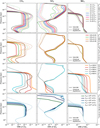 |
Fig. 2 VMR profiles of key species CH4, SO2, and NH3 in our grid of disequilibrium chemistry models of WASP-107b. Chemical equilibrium is plotted with thin, dashed lines. The nominal model of Z=10Z⊙, C/O=0.46, Tint=400 K, and log Kzz=9(cm2/s) was chosen to be in agreement with previous studies (Dyrek et al. 2024; Welbanks et al. 2024). |
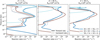 |
Fig. 3 Dominant reactions (by fastest reaction rate) that involve SO and SO2, for three different combinations of metallicity and eddy diffusion coefficient. Forward rates are shown by solid lines; backward rates by dotted lines. The other values of these simulations are Tint=400 K and C/O=0.46. |
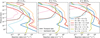 |
Fig. 4 Dominant reactions (by fastest reaction rate) that produce/destroy S, for three different metallicities. Forward rates are shown by solid lines; backward rates by dotted lines. The other values of the simulations are Tint=400 K, C/O=0.46 and log Kzz=9(cm2/s). |
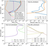 |
Fig. 5 VMR of SO2 and dominant H-producing reactions for a nominal model (Z=10 Z⊙, C/O=0.46, Tint=400 K, log Kzz=9 cm2/s) that includes all available photodissociation cross-sections (upper left panel), and three limiting cases where only the photolysis of one particular source is considered (N2, H2O., or NH3), copying the experiment of Dyrek et al. (2024). Panels that show thermochemical reaction rates show both their forward (solid lines) and backward (dashed) rates. |
3.2 Carbon chemistry: C2H2, CO, CO2, and CH4
From Fig. 2, it is clear that all four dimensions of the parameter space (Z, C/O, Tint, Kzz) impact the VMR profile of CH4. Furthermore, each panel shows the three well-known regimes from the top to bottom layers: photochemical destruction, transport-induced quenching, and thermochemical equilibrium. Aside from the general carbon budget, controlled by metallicity and carbon-to-oxygen ratio, the VMR of CH4 is mainly controlled by the VMR around the quench pressure, i.e. the point at which the chemical timescale matches the vertical mixing timescale.
The absence of abundant CH4 in WASP-107b has led to the suggestion of a tidally heated core (high Tint), in combination with strong vertical mixing (high Kzz) that quenches CH4 deep in the atmosphere and thus reduces the overall CH4 content in the observable layers (Fortney et al. 2020; Dyrek et al. 2024; Welbanks et al. 2024; Sing et al. 2024). This is also apparent from Fig. 6, which shows the quenched VMR and pressures of CH4 in our chemistry grid. At high Tint(>300 K), faster vertical mixing indeed quenches CH4 more deeply (higher pressure), resulting in an overall lower VMR. The opposite is true for low Tint(≤ 200 K), where we see that deeper quenching results in more CH4. This is due to a negative VMR gradient for layers in chemical equilibrium, as compared the positive gradient in models with high Tint (see also Fig. 2).
Furthermore, Fig. 6 shows an upwards shift in altitude (downwards in pressure) of the quench point at higher metallicity, together with an overall lower quenched VMR of CH4. The negative correlation between metallicity and CH4 is counterintuitive as one expects a positive correlation between the available carbon budget and eventual VMR of CH4. However, this is explained by Fig. 1, which shows that the deep layers are warmer at higher Z as a result by of the increased abundance (and thus opacity) of strong absorbers (Drummond et al. 2018). Additionally, chemistry in high-metallicity environments shifts the CH4−CO boundary to lower temperatures (Lodders & Fegley 2002). A warmer interior, for similar eddy diffusion coefficients, and high metallicity explain the upwards shift in altitude of the quench point, resulting in less CH4.
The formation of CH4 is coupled to CO, as both molecules can act as the dominant carbon reservoir under different circumstances. We find that in the majority of our models, CO dominates over CH4. Only in set-ups with (i) quasi-solar metallicity and/or (ii) shallow quenching by low Tint or weak Kzz, is CH4 more abundant than CO. For our nominal model of Z = 10 Z⊙, C/O=0.46, Tint=400 K, and log Kzz = 9 (cgs), we analyse the conversion pathway from CH4 to CO at the quench pressure and find
 (17)
(17)
 (18)
(18)
 (19)
(19)
 (20)
(20)
 (21)
(21)
 (22)
(22)
taking into account that OH is produced by Reaction (4). This pathway has been well documented in previous studies (Moses et al. 2011; Venot et al. 2012; Zahnle & Marley 2014; Tsai et al. 2017, 2018; Venot et al. 2020). Some of the above papers have reported dominant pathways that run via CH3OH, effectively replacing Reaction (18) with
 (23)
(23)
 (24)
(24)
for high-pressure (deep quenching) environments. We do not find a model in which this pathway is faster than Reaction (18). A faster pathway exists via COS, a stable sulphur molecule present in low amounts at chemical equilibrium (VMR < 10−7 in our nominal model), which produces CO via COS+CH3 → CO+CH3 S. However, COS itself is predominantly kept in equilibrium by reactions H+COS ↔ CO+SH and COS+SH ↔ CO+HS2, which both have CO as a reactant, disqualifying COS from the interconversion pathway CH4−CO. Finally, we find that multiple other pathways can come close to competing with the pathway of Reaction (22). This includes, for example, stripping CH4 to atomic carbon before oxidization to CO. We refer to Tsai et al. (2018) and Hu (2021) for a detailed description on the various CH4−CO pathways and regimes in which they occur.
Other carbon-species of interest are CO2 (detected in WASP-107b) and C2H2 (undetected). Production and destruction of CO2 is equilibrated by
 (25)
(25)
throughout the entire atmosphere across all dimensions of our model grid, and its VMR is hardly altered by disequilibrium chemistry (see Fig. A.1). However, we note photochemically produced OH has been shown to increase CO2 in some exoplanetary atmospheres (Moses et al. 2011; Zahnle & Marley 2014; Hu 2021). Finally, we briefly discuss C2H2 as it another important photochemical product in exoplanetary atmospheres (Line et al. 2010; Moses 2014; Baeyens et al. 2022; Konings et al. 2022). We find the average VMR of C2H2 to be below 10−10 in all our models, making it too scarce to be observable. We do note that its primary formation pathway in our models is well known, following CH4 → CH3 → C2H6 → C2 H5 → C2H4 → C2 H3 → C2H2, as was described in Moses et al. (2011).
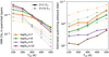 |
Fig. 6 Quenching VMR (left panel) and estimated quenching pressure (right panel) of CH4 versus intrinsic temperature Tint for various eddy diffusion coefficients in low (Z=1 Z⊙) and high (Z=10 Z⊙) metallicity atmospheres. The models with log Kzz = 6 (cgs) are not included as not all atmospheres are quenched at such weak vertical mixing. |
3.3 Nitrogen chemistry: HCN, N2 and NH3
Dyrek et al. (2024) reported a tentative detection of NH3 (2–3 σ) in WASP-107b at a VMR of ≲ 10−5.47, based on the 10.5 μm feature in the MIRI data. Subsequently, Sing et al. (2024) found marginal evidence of NH3, based on a 3 μm feature in the NIRSpec data. Most recently, Welbanks et al. (2024) could confirm the presence of NH3 with a 6 σ detection based on a panchromatic analysis covering both the 3 and 10.5 μm feature at ≲ 10−5 VMR, while also requiring an enhancement of a factor ∼30 to match the observed VMR to their best-fit forward model. This sparks an interest in the behaviour and chemical pathway of NH3 in our models.
Returning to Fig. 2, we observe only a slight dependency of NH3 on metallicity despite the linear dependence with the available nitrogen budget. Similarly to the behaviour of CH4, outlined in Sect. 3.2, one must take into account the PT profile and its vertical upward shift for higher metallicity as well as the shift in NH3−N2 balance (Lodders & Fegley 2002). Given the quasiconstant VMRs in the layers around the NH3 quench point, the upward (or downward) shift of the quench point altitude (or pressure) does not substantially affect the quenched VMR. A similar explanation can be given to the behaviour with respect to Kzz as a stronger eddy diffusion coefficient, and thus deeper quenching, does not affect the quenched NH3 VMR too much due to quasi-constant VMRs in chemical equilibrium (Moses et al. 2011; Moses 2014).
Similar to the CH4−CO interconversion described in Sect. 3.2, the ratio between NH3 and N2 is frozen at the quench point and sets the dominant nitrogen reservoir in the middle atmosphere. From Fig. 7, it is clear that a higher intrinsic temperature results in a lower quenched VMR of NH3 as the quench point moves up in altitude. Additionally, the minimal dependence on metallicity and Kzz is clearly shown here as well.
In all of our chemistry models, we find a clear overabundance of N2 with respect to NH3 by several orders of magnitude. Only in a limiting case with Z = 1 Z⊙, Tint = 100 K, and high Kzz, the overabundance of N2 is limited to a factor two. We identify the primary pathway for NH3−N2 conversion as
 (26)
(26)
 (27)
(27)
 (28)
(28)
 (29)
(29)
 (30)
(30)
 (31)
(31)
around the quench pressure, which is in agreement with the literature (Moses et al. 2011; Hu 2021). An alternative pathway can replace Reaction (28) with
 (32)
(32)
 (33)
(33)
at higher quenching pressures but fails to be the quickest way to form N2 from NH3 in our models.
A final nitrogen-species of potential interest is HCN, as photochemistry can enhance its presence significantly from chemical equilibrium (Baeyens et al. 2024). However, HCN remains undetected in WASP-107b, and is not expected to be prominent in transit spectra at this temperature regime (Baeyens et al. 2022). In our models, HCN reaches an maximal VMR of ∼10−6 in some limiting cases (see Fig. A.1). It forms primarily from the net reaction CH4+NH3 → HCN+3 H2, after hydrogen abstraction of both reactants (Moses et al. 2011), thus depending heavily on their abundance in the atmospheres.
4 1D-RCPE retrievals of WASP-107b
In this section, we run retrievals based on the grid of 1D-RCPE models. We start by briefly discussing the main molecular features in cloud-free transit spectra (Sect. 4.1). In Sect. 4.2, we fit with a simplified ‘grey’ cloud set-up for transit observations below 5 μm to gradually build up our understanding of the 1D-RCPE retrieval method. Afterwards, in Sect. 4.3, we combine all information of the previous sections and run retrievals with complex non-grey clouds on all available observations. For both Sects. 4.2 and 4.3, we present a nominal case in which the results serve as a benchmark.
4.1 Transmission spectra
With a thorough understanding of the chemical processes and pathways, we are equipped to transform these models into observables. As is described in Sect. 2, we computed transmission spectra of our models on the fly during the fitting routine. Fig. 8 shows cloud-free transmission spectra that probe the parameter space of our grid.
A number of molecular features show a clear variation in amplitude. The spectra are dominated by several broad H2O bands, a distinct SO2 bump around 4 μm and a double SO2 feature at 7–9 μm, a CO2 feature at 4.3 μm (and contribution at 2.8 μm), a small CO bump around 4.6 μm, and a narrow-peaked CH4 feature at 3.4 μm. Note that the latter molecule has broad bands and can dominate the spectra in more methane-rich models. The VMRs of CO2, CO, H2O, and SO2 all scale with metallicity to a certain degree and can therefore provide more opacity in the observable layers at higher metallicity. At the same time, a high-metallicity atmosphere is more compact due to the increased mean molecular weight, which tends to reduce feature amplitudes as the scale height decreases. Although both effects counteract each other, the upper panel of Fig. 8 shows a clear positive correlation between feature amplitude and metallicity. The opposite is true for CH4(3.4 μm), for which the VMR decreases with metallicity (also see Fig. 2) but the feature strength remains the same for all considered metallicities.
At low C/O, less CH4 is present in the atmosphere and more oxygen is stored in SO2 and H2O, compared to CO and CO2. As a result, a sub-solar C/O gives a weaker CH4 feature and more pronounced SO2 and H2O bands. Models with high Tint generally have less CH4 and NH3, which is directly visible in Fig. 8. The CH4 feature at 3.4 μm diminishes in amplitude at higher Tint. In general, we do not see substantial contribution of NH3 in these cloud-free spectra, with the exception around 10.5 μm in the models with the lowest Tint.
Finally, we briefly discuss the bottom panel of Fig. 8, where different values of Kzz are explored. While higher Kzz results in deeper quenching, and an overall lower amount of CH4 in the bulk atmosphere, the effect on the spectral feature at 3.4 μm is small. The SO2 features around 7–9 μm scale with Kzz, which is easily explained by its VMR in the upper layers. At higher Kzz, vertical mixing is more efficient in replenishing the upper layers with SO2 as it competes with the photochemical destruction. Given the high transit depth of these SO2 features, it is sensitive to exactly these upper layers in the chemistry models, which explains its behaviour in the spectrum. As we shall see later, the same mechanism can affect the 3.4 μm feature of CH4, especially in the presence of a high altitude cloud deck that blocks the bulk CH4 content below from forming a stronger spectral feature. We emphasize that Fig. 8 was computed for cloud-less spectra, whereas the next sections include clouds that substantially affect the (amplitude of) visible molecular features.
4.2 Retrievals with grey clouds on transit spectra below 5 μm
We proceed by fitting our grid of 1D-RCPE models to HST (Kreidberg et al. 2018) and JWST’s NIRCam (Welbanks et al. 2024) observations of WASP-107b. In this wavelength range, we can highly simplify the cloud treatment and avoid the discussion on more complex (silicate) clouds for now. The most simple parametrization of a cloud deck can be achieved by applying a grey opacity with a base on certain pressure (Pcloud). We ran our fitting routine (described in Sect. 2.8) on JWST’s NIRCam and HST data and allow for an offset between the two (ΔHST). We included the full range of grid parameters for Z(1 to 30 Z⊙), C/O(0.05 to 0.46), and Tint(100 to 500 K), with the exception of Kzz(107 to 1010 cm2/s). We excluded models with Kzz=106 cm2/s as these atmospheres are not always quenched in our grid, which makes a linear interpolation between such models inconsistent. Finally, we fitted a reference pressure (Pref) at the planetary radius, which gives a total of seven free parameters (Z, C/O, Tint, Kzz, Pref, ΔHST, and Pcloud) with flat priors that were fitted for.
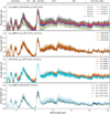 |
Fig. 8 Cloud-free synthetic spectra of our grid of 1D-RCPE models for WASP-107b computed with petitRADTRANS. The top row indicates the dominant opacity sources, with secondary contributors in brackets. |
4.2.1 Results of the nominal retrieval: Case 1
Fig. 9 shows the best-fit spectrum of our nominal retrieval (Case 1), summarized in Table D.1. By analysing the order of convergence, we see that the metallicity  and
and  are constrained the easiest, together with offset parameters Pref and ΔHST. Upon closer examination (Fig. B.1), a degeneracy exists between Z, Pref, and Pcloud due to the dominant presence of H2O, both due to the amount of spectral features and high VMR, and the strong feature of CO2 at 4.3 μm. Depending on the metallicity, and thus overall H2O and CO2 content, one can vary both Pcloud and Pref to correctly match the scale height of these features. Note that an increased metallicity affects the spectrum in two ways. First, the amplitude of the many H2O features (and CO2) will scale with their abundance, which can be fitted with a vertical offset (controlled by Pref) to match the top of the feature and Pcloud, which blocks the layers below. Second, an increased metallicity also implies a higher overall mean molecular weight. This effectively decreases the pressure scale height and hence the physical extent of the atmospheric layers through which star light is absorbed. This reduces the amplitudes of all spectral features, including those of H2O and CO2, and has a similar effect to fitting a high-altitude cloud deck (low Pcloud). It is the 4 μm SO2 feature that breaks this degeneracy, despite slightly underestimating the transit depth in this region, as SO2 is highly sensitive to metallicity. In Sect. 4.3, we further discuss the ability of SO2 features to constrain metallicity.
The constraint of Pcloud to low pressures is crucial for the retrieval of  , and
, and  (cgs). The most straightforward explanation of such low C/O would be that an extremely carbon-poor atmosphere removes excessive CH4 that would otherwise dominate the full wavelength range. However, also oxygen-rich species are affected by such low carbon-to-oxygen ratios. Compared to a solar C/O, there is also less CO2 and more H2O, which are both dominant contributors in these spectra. Fitting the relative proportion between both H2O and CO2 features cannot be done by adjusting the general metallicity. Instead, one must lower the carbon-to-oxygen ratio to downscale the CO2 feature with respect to the H2O bands, which explains the preference towards such low C/O value.
So far, we have not discussed the 3.4 μm CH4 feature that is fitted nicely by our retrieval. Other than a sub-solar C/O, we stated in Sect. 3.2 that a combination of high Tint and high Kzz causes deep quenching and a low CH4 abundance (Fig. 6). However, we fit our grid to a very low Tint, which leaves a large amount of methane in the atmosphere (see Fig. 2). Fig. 9 also shows the very limited impact of Tint on the spectrum for this combination of Z, C/O and Pcloud. We find no substantial difference (< 20 ppm) across the full prior range of considered intrinsic temperatures, a very peculiar result considering our findings in Sect. 3.2 (Fig. 6). However, by fitting the cloud deck at Pcloud ≃ 10−3.54 bar, one effectively shields the layers below where the bulk methane is present. One still needs to fit the 3.4 μm methane feature in some way, which is achieved via the vertical mixing parameter Kzz. Although a larger value for Kzz implies deeper quenching, and thus a lower quenched VMR, it has a different effect in the upper atmosphere. There, it competes with photochemical destruction to mix additional CH4 in the upper layers. Given the high-altitude cloud deck that is retrieved exactly around these layers, the retrieval algorithm prefers models with high Kzz to provide the necessary amount of methane that can fit the 3.4 μm feature. This is also in agreement with a lower Tint, as this sets the bulk amount of methane beneath the cloud deck, which is mixed upwards. Note that this explanation does not contradict our findings of Sect. 3.2, as the situation is drastically affected by the cloud deck. This means that, in this particular case, parameters Tint and Kzz were fitted to maximize the CH4 feature at 3.4 μm instead of minimize it.
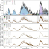 |
Fig. 9 Best-fit spectrum of Case 1 with molecular contributions (upper panel). The bottom panels show spectra within 1σ, 2σ, and 3σ uncertainty levels of the mean posterior values. The data plotted in the upper panel consists of HST WFC3 (Kreidberg et al. 2018) and JWST NIRCam (Welbanks et al. 2024). |
4.2.2 Sensitivity analysis: Cases 2, 3, 4, 5, and 6
We continue with the same retrieval set-up, but now we systematically fix a parameter beforehand and exclude it from the run. In this way, we enhance our understanding of the 1D-RCPE retrieval method and demonstrate how our results are influenced by variations in the specific model parameters. The results of these retrievals are summarized in Table D.1. When assuming Z=10 Z⊙ (Case 2) based on previous findings (Welbanks et al. 2024; Dyrek et al. 2024), we find a different result compared to our nominal retrieval (Case 1). Due to the strong presence of the CO2, SO2, and H2O features at this metallicity, the cloud deck was placed at a higher altitude (lower Pcloud) to reduce their amplitudes. Note that the reference pressure, Pref, was adjusted accordingly, being degenerate with Pcloud and metallicity. Our retrieval constrains Kzz to a value close to the lower boundary of the prior (<107.5 cm2/s). This is again a peculiar result given the fact that previously we found that the high cloud deck requires a higher Kzz value to mix sufficient amounts of CH4 into the upper layers to form a visible spectral feature. However, the same upward mixing also affects other species such as H2O, CO2, and in particular SO2. After fixing Pcloud based on the high metallicity, the retrieval minimizes Kzz to further reduce the scale height of these features. We note that the carbon-to-oxygen ratio is, again, fitted based on the relative amplitude of the CO2 and H2O bands, which explains the extremely low value. Finally, we note that Tint remains unconstrained, as the combination of high clouds and low Kzz prevents any amount of methane from being visible in the upper layers. The overall fit is of a much lower quality than the nominal model ( compared to 2.18 for Case 1). The reason is twofold as (i) no combination of Z, Pref and Pcloud can sufficiently reduce the 4 μm SO2 feature and (ii) the low value of Kzz prevents CH4 from forming a feature at 3.4 μm above the cloud deck.
Running the retrieval with a fixed solar C/O (Case 3), gives  and
and  . By fixing the C/O beforehand, and thus the relative amplitude between the H2O and CO2 features, a slightly lower metallicity is preferred to fit these features. This is a consequence of the nonlinear relation between the VMR of CO2 and Z, while H2O does scale linearly with metallicity. Towards higher metallicities, the increase in CO2 is greater than H2O, requiring a much lower C/O to fit the resulting feature amplitudes. Note that this results in a poor fit of the SO2 feature, as there is none at such low metallicity in these spectra. The slightly lower value for Z results in a deeper cloud deck (higher Pcloud), as there is less of a need for these high clouds to reduce the amplitudes of the spectral features. These relative deep clouds now expose more layers containing a substantial CH4 content, which in turn explains the extremely high Tint and low Kzz. We repeat that, although a low Kzz results in more shallow quenching (Fig. 6), there is less methane mixed in the upper (visible) layers (see Fig. 2).
Another exercise is to fix Tint=500 K (Case 4), a parameter that is typically constrained with great difficulty as it only affects the 3.4 μm CH4 feature. The retrieval first finds a solution between the metallicity, Pref, and Pcloud, after which it converges to a sub-solar C/O and low Kzz. Interestingly, both Z and C/O are much less tightly constrained than before, encompassing the values of Case 1 within the 1 to 2 σ level. As a high Tint does not affect the VMR of H2O, CO2, or SO2, the only difference stems from starting with a fixed Tint that affects the VMR of CH4. When we fix log Kzz=10 (cgs) in Case 5, we find results that closely resemble our nominal model with no fixed parameters (Case 1). Do note the exception that a slightly higher intrinsic temperature is fitted for, which removes additional CH4, as more material gets mixed in the upper observable layers as a result of the higher Kzz. The BIC values for Case 4, and especially Case 5, are close to that of the nominal model (Case 1). This confirms that Tint and Kzz are less important for the retrieval outcome compared to Z and C/O, as they are more difficult to constrain.
Finally, we fixed the cloud deck to Pcloud=10−3 bar (Case 6), which is deeper in the atmosphere than has been previously fitted for. As usual, this directly affects the metallicity (and Pref), which was now fitted to a relatively low value of  as there was no high cloud deck to reduce the scale height of the spectral features. We find a slightly higher C/O compared to other runs, which is a result of fitting a lower Z that affects the relative VMR of CO2 with respect to H2O. Again, this lower Z affects the quality of fit as the SO2 bump at 4 μm is not fitted well. The deep cloud deck fails to block the CH4−rich layers. Therefore, a combination of high Tint and low Kzz minimizes the CH4 opacity contribution to the spectrum, explaining the final results.
4.2.3 A wavelength-dependent opacity slope: Case 7
A consistent result among all runs is the very low C/O value. The retrievals achieve these values by trying to reduce the CO2 feature (4.3 μm) in amplitude with respect to the H2O band (2.5–3.0 μm) or vice versa. Rayleigh scattering can introduce a slope towards the optical part of the transit spectrum, effectively altering the fit for the HST data (and thus ΔHST). Given the detection of larger silicate droplets in WASP-107b (Dyrek et al. 2024), a non-Rayleigh type of short-wavelength absorption could be present that follows a much more shallow wavelengthdependence. In Case 7, we fit for a free slope and find  , which is more indicative of Mie scattering caused by mid-sized to larger aerosols. The effect on C/O is minimal, however, as we retrieve a similar value as before. We do obtain a better fit compared to the nominal model (Case 1), as well as a better BIC, indicating that this retrieval manages to explain the data better. Note that Pcloud loses its meaning as the opacity source with the shallow slope now replaces the grey cloud deck (Pcloud). Therefore, in future simulations with a fitted γscatt, we do not fit for Pcloud.
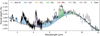 |
Fig. 10 Best-fit spectrum for Case 10. The data plotted in the bottom panel consists of HST WFC3 (Kreidberg et al. 2018), JWST NIRCam (Welbanks et al. 2024), and JWST MIRI/LRS (Dyrek et al. 2024). |
4.2.4 Information content of HST and JWST NIRCam data: Cases 8 and 9
Finally, we briefly consider different combinations of datasets in these retrievals with grey clouds, excluding the JWST MIRI data of WASP-107b for now. A fit to the HST dataset alone (Case 8) only constrains a high cloud deck, as no features other than of H2O are visible. In particular, the metallicity remains unconstrained, which provides further evidence that features from only H2O are not sufficient to constrain Z. Furthermore, fitting to the NIRCam dataset separately (Case 9) gives similar results as to fitting it in combination with HST data (Case 1). We conclude that, as expected (e.g. Edwards et al. 2023), the retrieval needs a feature-rich spectrum such as JWST NIRCam to constrain atmospheric properties.
4.3 Retrievals with non-grey clouds on transit spectra up to 12.2 μm
Observations with the JWST MIRI instrument (LRS) provide us with additional wavelength coverage up to ∼12.2 μm. Given the additional opacity source between 8 and 10 μm, stemming from (silicate) clouds (Dyrek et al. 2024; Welbanks et al. 2024), we ran retrievals with non-grey cloud parametrizations described in Sect. 2.6. We included uniform priors that span the entire range of the four grid parameters (Z, C/O, Tint, Kzz) with the exception of log Kzz=6 (cgs) as we only want to include quenched atmospheres. Next to an offset with HST data (ΔHST), we also fitted an offset with the NIRCam data (ΔNIR) in reference to the MIRI data. Together with the model offset (Pref), this makes a total of seven free parameters without the cloud treatment.
4.3.1 Results with Gaussian clouds: Cases 10, 11, 12, 13, and 14
We started by adopting the cloud parametrization of Welbanks et al. (2024), which introduce three more fitting parameters (κopac, λ0, ω) as we fixed ξ = 0 after initial testing to reduce the computational cost. Additionally, we included a wavelength-dependent opacity slope as described in Eq. (2), which introduces two additional fitting parameters to the retrieval (κscatt, γscatt). Note that we do not fit for a grey cloud deck (Pcloud) if we consider γscatt in the retrieval.
Figs. 10 and B.2 show the best fit spectrum marginal posterior distributions of this retrieval (Case 10). Overall, we achieve a good fit for all datasets with the exception of the noisy region above 10 μm. At 4 μm, we find that our best-fit model contains mostly SO2 opacity, although it does not reproduce the narrow peak in the data completely. As is established in Sect. 4.2, the metallicity is degenerate with the model offset (Pref) and cloud opacity (e.g. Pcloud) when fitting to the H2O and CO2 features in the transit spectrum below 5 μm. Only the 4 μm feature of SO2 helps constrain the metallicity as higher values for Z (and thus higher VMR of SO2) would result in a SO2 feature with too high amplitude. Interestingly, the inclusion of two broad SO2 features around 7–9 μm does not change the retrieved metallicity ( significantly compared to previous retrievals with grey clouds (
 , see Table D.1). This could indicate that any of the SO2 features are a robust indicator of atmospheric metallicity, or that the Gaussian cloud feature is degenerate with the SO2 features at 7–9 μm, and thus metallicity is constrained only on the 4 μm SO2 feature.
If SO2 is a strong indicator of the metallicity in a photochemically active atmosphere, its features in the MIRI data should cause the retrieval to converge to a similar value for Z. Indeed, re-running the retrieval without HST and NIRCAM data (Case 14, with Pcloud instead of γscatt) results in  , which is within the 1 σ level as before (Case 10). Further investigation confirms that the quality of fit decreases with a fixed higher metallicity (see BIC of Case 11 with Z=10 Z⊙ in Table D.2). We conclude that the SO2 features, either at 4 μm or 7–9 μm, are robust features to constrain the metallicity. In Sect. 5, we further discuss their dependence on model assumptions such as the temperature in the upper layers.
The inclusion of MIRI data introduces features of two oxygen-bearing species (H2O and SO2) and (a lack of) one carbon-bearing molecule (CH4), which can further impact the C/O. We find that the nominal retrieval (Case 10) has difficulties constraining C/O (next to Tint and Kzz) compared to other parameters such as Z, Pref, and the cloud properties. Similar to our findings before (Sect. 4.2), we find that the easy constraints on cloud (and scattering) opacity affect the further convergence of C/O. As the high-altitude layer of aerosols shields the layers with substantial CH4, and thus the formation of any features in the spectrum, the  is constrained by the relative amplitude of the 4.3 μm CO2 feature with respect to features of oxygen species (e.g. H2O and SO2 in NIRCAM). Within the MIRI data, lowering the C/O effectively reduces the amplitude of both SO2 and H2O feature as no carbon-species has a strong feature. Therefore, we find that the C/O is still mainly controlled by the 4.3 μm CO2 feature. To further assess the sensitivity of C/O to the scattering treatment, we run the same retrieval without scattering and find a marginally lower C/O of
  (Case 13, Table D.2). Furthermore, a simulation with a fixed solar C/O gives a satisfactory fit (see BIC of Case 12 in Table D.2), indicating that an adjusted low-wavelength opacity slope can reduce the need to fit a low C/O. We carefully conclude that the above indicates a degeneracy between C/O and the wavelength-dependent opacity slope.
Parameters Tint and Kzz are least constrained by the retrieval. We find a relatively high intrinsic temperature of  and intermediate log Kzz of
  . As was previously established, a high-altitude cloud deck shields the CH4−rich layers and prevents it from forming features in the observable spectrum. Once again, this hypothesis is confirmed by finding no substantial difference (< 15 ppm) between model spectra across the full range of Tint, while otherwise adopting the best-fit values. The CH4 feature at 3.4 μm is fitted by increasing Kzz so that additional CH4 is mixed upwards and reaches above the cloud deck. While Tint mostly affects CH4 features in the transmission spectrum, we do note that Kzz also affects the abundances of SO2 and CO2 (e.g. Fig. 2 and Fig. A.1), and therefore also the scale height of their spectral features.
Finally, we note that none of the above fits contain a significant contribution from NH3, a species detected by Welbanks et al. (2024) at 3 μm (and 10.5 μm to a lesser extent) in WASP107b. Although we do not obtain a good fit overall above 10 μm with our models, the region around 3 μm is well fitted by mostly H2O opacity instead of NH3. As is discussed in Sect. 3.3 and shown in Fig. 2, NH3 is most abundant in atmospheric models with low Tint. Similar to CH4, high altitude clouds could obscure NH3−rich layers and limit the amplitude of any potential spectral features. Meanwhile, at a high Kzz additional material could be mixed upwards above the cloud deck and become visible in the transit spectrum. However, we do not find substantial opacity contributions of NH3 in cloud-free models (Fig. 8). To further investigate the impact of NH3, we run a retrieval with Gaussian clouds and a wavelength-dependent opacity slope (Similar to Case 10) without NH3 opacity in the radiative transfer computation. We find that this does not affect the retrieval outcome and conclude that NH3 opacity does not play a role in any of the above retrievals.
4.3.2 Retrievals with silicate condensate clouds: Cases 15, 16, and 17
Given the detection of silicate condensates in the MIRI data (Dyrek et al. 2024), we run retrievals that use optical properties of SiO, SiO2, or MgSiO3 to explore their effect on other fitting parameters. As is detailed in Sect. 2.6, this introduces four more parameters  ) as we fix xσ=−1. Next to the four grid dimensions (Z, C/O, Tint, Kzz) and three offsets (Pref, ΔHST, ΔNIR), this totals 11 fitting parameters. Note that the implementation of particle size and mass fraction distribution removes the need for separate parametrized scattering. As expected, we retrieve metallicities and carbon-to-oxygen ratios that are in line with previous runs, confirming that both these parameters are not sensitive to the way we choose to parametrization clouds in our set-up. In contrast to our results with Gaussian clouds, we now find lower intrinsic temperature (≲ 250 K). In line with our previous findings, a low Tint is caused by the altitude at which the aerosols become optically thick and whether or not this exposes the CH4−rich layers. Another notable difference with the Gaussian cloud parametrized retrievals is the quality of fit, which is much lower in this case. Closer inspection reveals that the JWST MIRI data is not properly fitted for (Fig. C.1), which confirms that a single silicate species cannot explain the broad 8 to 10 μm cloud feature (Dyrek et al. 2024). Although determining which (combination of) silicate cloud species or other condensates can fit the data better is out of the scope of this study, we briefly discuss the debated presence of silicate clouds in Sect. 5.3.
5 Discussion
In this section we discuss the implications of our results for WASP-107b. First, we discuss our findings on the elemental composition (Z and C/O) in Sect. 5.1 before discussing the reason why our retrievals cannot constrain Tint and Kzz properly in Sect. 5.2. Finally, we review the presence of high-altitude clouds that consist of silicates particles in Sect. 5.3.
5.1 Retrieved composition of WASP-107b
We consistently find metallicities of 3–5 Z⊙ in retrievals that achieve a good fit. As is discussed extensively in Sect. 4, the metallicity is constrained based on the SO2 features at 4 and 7–9 μm as SO2 production is dependent on the available sulphur (H2S) and oxygen reservoirs (H2O) (see Sect. 3.1). Sulphur dioxide effectively breaks the degeneracy between metallicity (based on features of H2O, and CO2), model offset (fitted Pref at Rpl), and top of the cloud deck (Pcloud). Our derived metallicities are lower than values reported in the literature, which range between 10 and 18 Z⊙ (Welbanks et al. 2024) and 43 ± 8 Z⊙ (Sing et al. 2024). As SO2 is a photochemical product, its VMR profile is determined by (i) the SED emitted by the host star (in particular the UV), and (ii) the temperature structure (Tsai et al. 2023; Dyrek et al. 2024; de Gruijter et al. 2025). We note that Welbanks et al. (2024) use the same SED (HD 85512 from the MUSCLES survey) as we do in this study. Therefore, we attribute part of the difference in derived metallicity to their lower upper-layer temperature (450–550 K) with respect to ours (650–750 K). At lower temperature, the thermochemical conversion from H2O into OH (Reaction (4)) becomes slower, which suppresses the efficiency of sulphur oxidization (e.g. Reaction (8)). Hence, a higher metallicity is required to produce sufficient SO2 in their models.
The strong sensitivity of SO2 to temperature inspires us to revisit an assumption made in the construction of PT profiles (Sect. 2.2). By fixing rst = 1 (effectively a dayside average PT structure), we computed a profile with a quasi-isothermal upper atmosphere of 650–750 K while setting rst = 0.5 (planetwide average) would lower this by ∼100 K. To test the effect of this assumption on our results, we ran an additional grid of 900 models with these slightly cooler PT profiles. We then ran retrievals using the same set-ups as Case 1 (Table D.1) and Case 10 (Table D.2); we present the results in Table D.4. We find metallicities of  (Case 18) and
  (Case 19), respectively, which indicates only a marginal increase in retrieved metallicity compared to our initial retrievals with rst=1. Fig. 11 shows the best-fit spectrum of Case 19 and Case 10, as well as the PT profiles and VMRs of key species. Despite a general decrease in SO2 in the upper regions, a similar fit can be achieved by leveraging the Rpl–Pref degeneracy and cloud opacity. This indicates that the predictive power of SO2 for metallicity indeed depends on the assumed temperature in the upper layers. What further complicates the correct estimation of the upper layer temperature is the fact that observations do not probe a 1D atmosphere and thus we cannot assume a uniform temperature on the terminator region. A slight asymmetry between the evening and morning limb has been detected on WASP-107b, resulting from a ∼100 K difference (Murphy et al. 2024). Limb asymmetry not only affects the temperature and chemistry but changes the scale heights as well, which can bias the observed transit spectrum (Caldas et al. 2019; Falco et al. 2022; Pluriel et al. 2022; Lee et al. 2022; Nixon & Madhusudhan 2022).
Another consistent finding of our retrievals is the carbon depletion with respect to oxygen (C/O), typically in the range of 0.10 to 0.20. We find that this parameter is mainly determined to the relative amplitude of the 4.3 μm CO2 feature with respect to broad features of oxygen species, in particular H2O. If the retrieval of this parameter is reliant on a single CO2 feature, one must question the relatability and investigate the underlying chemistry that produces CO2. As is detailed in Sect. 3.2, we find that the VMR of CO2 is mainly set by thermochemistry and is less sensitive to disequilibrium effects in our models of WASP-107b. Retrievals with cooler upper layers (rst=0.5) prefer models with a slightly lower C/O (Table D.4), indicating an even higher carbon depletion is needed to fit the spectra properly.
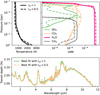 |
Fig. 11 Best-fit PT profile (upper left), VMRs of key species (upper right), and model spectra (bottom) of retrievals Case 19 and Case 10 that have Gaussian clouds and a free wavelength-dependent opacity slope. The grid of models used for Case 19 are approximately 100 K cooler in the isothermal layers (rst=0.5) compared to those used for Case 10(rst = 1). Note that both retrievals converge to a different set of grid parameters (Z, C/O, Tint, Kzz), which affects the VMRs and PT profiles, but a fit of similar quality can be achieved. |
5.2 High-altitude aerosols can shield CH4−rich layers
We retrieve intrinsic temperatures that span the entire range of our priors (100 to 500 K). Together with Kzz, our retrievals struggle to constrain Tint and both parameters often have large uncertainties. We attribute the large spread in Tint values to high-altitude clouds that block the layers below from forming spectral features, like the 3.4 μm CH4 feature. Additionally, we find that strong mixing can mix material above the cloud deck so that a higher Kzz implies a stronger feature. This is counter-intuitive from a chemical standpoint, which shows that stronger mixing results in deeper quenching of CH4 and thus lower VMR (Fig. 6). We conclude that the feature at 3.4 μm is fitted by a delicate balance of Pcloud (or equivalent aerosol opacity) and Kzz, while Tint is less important than expected.
Previous studies have suggested that a high intrinsic temperature, in combination with deep quenching by efficient vertical mixing, is responsible for the lack of abundant methane in WASP-107b (Kreidberg et al. 2018; Fortney et al. 2020; Dyrek et al. 2024; Welbanks et al. 2024; Sing et al. 2024). In particular, Welbanks et al. (2024) constrains Tint>345 K and log Kzz = 8.4–9.0 cm2/s, which our retrievals reproduce when a similar set-up is used (Case 10, Table D.2). Although this paper shows that these results can vary with different modelling choices and retrieval set-ups, we can neither confirm nor reject the high internal temperature scenario for WASP-107b. A hot interior is consistent with the highly inflated radius and low density, likely caused by tidal inflation (Leconte et al. 2010; Fortney et al. 2020; Welbanks et al. 2024), and the suggested presence of high-altitude silicates (Dyrek et al. 2024). Instead, we argue that hybrid retrieval approaches must be interpreted with caution and their robustness verified against various assumptions.
The delicate balance between Tint, Kzz, and clouds relates directly to the underlying grid of forward models. If the cloud deck is fitted slightly deeper in the atmosphere, and more CH4 is exposed to the observable layers, the retrieval tends to maximize Tint and minimize Kzz, while the opposite is true for a slightly higher cloud deck. This behaviour could be a consequence of the disconnect between our treatment of disequilibrium chemistry and post-processing of clouds in the radiative transfer. In particular, it can be expected that the methane homopause is shifted upwards as high clouds act as an additional UV absorber, shielding lower layers from photochemistry and increasing local heating rates (Molaverdikhani et al. 2020; Sánchez-Lavega et al. 2023). Additionally, clouds affect the gas-phase chemistry (Mahapatra et al. 2017; Helling 2019; Kiefer et al. 2024), which in turn also affects the PT structure (Marley et al. 2013; Lee et al. 2024). This calls for a general framework that allows feedback between (kinetic) cloud formation, gas-phase disequilibrium chemistry, and radiative transfer.
Finally, we note that other processes can deplete CH4 as well. Zonal quenching can be induced by equatorial mixing (Bell et al. 2024), although this effect could be small for WASP-107b (Baeyens et al. 2021). Furthermore, vertical mixing is treated as eddy diffusion, which assumes length scales that are much smaller than the pressure scale height, thereby mimicking diffusion (Tsai et al. 2017). However, given the potentially large interior temperatures and resulting steep temperature-pressure gradients, a large part of WASP-107b’s atmosphere could be dominated by convective energy transport. Therefore, additional large-scale mixing might take place that is not captured by the constant eddy diffusion coefficients (Baeyens et al. 2021).
5.3 Silicate clouds at high altitudes
Dyrek et al. (2024) report a statistical preference for silicate species SiO, SiO2, and MgSiO3 with respect to a simpler cloud set-up. Particularly notable is the high altitude at which the silicate cloud deck was retrieved, while condensation of such silicates occurs at high temperatures (e.g. 1200–1500 K) (Lodders & Fegley 1999; Visscher et al. 2010) and thus much deeper in the atmosphere. Given this expected deep condensation, Welbanks et al. (2024) show that vertically extended clouds are required to become visible in the transit spectrum (fsed < 0.5). However, the resulting small particles give an unsatisfactory fit to the observations. Dyrek et al. (2024) find a good fit with large silicate particles (fsed>3) so that the question remains how such a compact cloud deck of large aerosols can be suspended at high altitudes, far above the expected condensation region. One possibility is that efficient vertical mixing can loft particles to high altitudes continuously before they grow large and settle down. Given the intermediate value for fsed that Dyrek et al. (2024) find, atmospheres with high Kzz would require particles to grow large quickly and form a relative compact cloud at such high altitudes. WASP-107b’s low gravity could facilitate this slow settling and maintain high-altitude silicate clouds.
Although the focus of this study is to assess the robustness of retrieval outcomes against different assumptions, including the cloud parametrization, we briefly put our results in context of the above. In retrievals with individual silicate cloud species, we find fsed values roughly between 1.50 and 3, moderate values for  , and relatively high altitudes of the cloud pressure (Pcloud). This supports the case of a high-altitude thin cloud deck composed of moderate-sized particles, although this challenges the hypothesis of strong vertical mixing that replenishes these layers and reduces the sedimentation efficiency. When fitting with Gaussian clouds and a wavelength-dependent opacity slope (Welbanks et al. 2024), we retrieve
  (Case 10). The absence of a steeper scattering slope (e.g. γscatt = −4) indicates that sub-micron particles are not dominant in the atmosphere. Instead, the fitted shallow slope resembles more Mie-type scattering, caused by particles with comparable sizes to the photon wavelength, supporting larger grains of one to several micron.
6 Summary and conclusion
In this paper, we have conducted an in-depth study on the performance and reliability of 1D-RCPE retrievals on transmission spectra of WASP-107b. We have built a grid of 900 atmospheric models that take into account radiative heating, convection, vertical mixing, and thermo- and photochemistry and explore a range of different metallicities, carbon-to-oxygen ratios, intrinsic temperatures, and eddy diffusion coefficients. We have analysed the behaviour of WASP-107b’s gas-phase chemistry against different parameters and mapped important chemical pathways for key species in the atmosphere. We have subsequently used a nested sampling algorithm to perform Bayesian inference on archival datasets of WASP-107b and assessed the robustness and reliability of our outcomes against different cloud treatments.
Below, we summarize our main findings on the chemistry in our models of WASP-107b. The main formation pathway of SO2 in WASP-107b is through oxidization of atomic sulphur or H2S+2H2O → SO2+3H2, with variations at a high atmospheric metallicity involving oxidization of di-atomic sulphur (S2) and/or direct combination of two SO compounds into SO2. Hydroxide radicals are available due to hydrogen abstraction and photolysis of H2O. Atomic sulphur is typically liberated by hydrogen abstraction of H2S. The production of SO2 is therefore also sensitive to atmospheric metallicity. Furthermore, we explain how photolysis of non-hydrogen-bearing species such as N2, in the absence of other photon absorbers, can interact with the H2 reservoir to enable additional SO2 production. Regarding CH4, we reproduce the well-known CH4−CO conversion pathway via hydroxy-methyl (CH2OH) that affects the quenching pressure and VMRs deep in the atmosphere. We find a negative correlation between the quenched CH4 content and atmospheric metallicity due to the additional heating of the deep layers. At high Tint, we find that strong mixing (Kzz) results in deep quenching and decreases the quenched VMR of CH4, while the opposite is true for models with low Tint. Finally, we find that NH3 quenching occurs much deeper in the atmosphere and is less sensitive to Kzz due to the steep temperature gradient around the quenching point.
Below, we summarize our main findings of the 1D-RCPE retrievals:
We find that SO2 features at 4 and 7–9 μm are most informative to determine the atmospheric metallicity, which is consistently retrieved to be between 3 and 5 Z⊙ in retrievals that achieve a good fit. This is the case when we consider JWST NIRCam data separately, for JWST MIRI/LRS data if the 10 μm silicate cloud feature is taken into account, or a combination of both. We note that the amplitude of the SO2 features is, next to the stellar SED, dependent on the assumed temperature in the upper layers as this affects the available hydroxide that oxidizes Sulphur;
In the absence of strong SO2 features, we find a degeneracy between metallicity, the fitted reference pressure, Pref, and the altitude of the clouds (Pcloud). This is because the latter two parameters can control the feature amplitude regardless of the VMRs of dominant absorbers such as H2O and CO2, which scale with Z;
The carbon-to-oxygen ratio (C/O) was fitted to sub-solar values (≲ 0.20) based on the relative amplitude of the large 4.3 μm CO2 feature with respect to broad bands of H2O (and SO2), and much less to the 3.4 μm CH4 feature as the latter is often shielded by high-altitude clouds. This sensitivity highlights the need to properly model the VMR profile of CO2, which is sensitive to thermochemistry for WASP-107b and disequilibrium chemistry in some other cases;
In general, we find a slightly higher C/O when a wavelength-dependent opacity slope is included that mimics scattering towards the optical transit spectrum. The main reason for this is that such opacity increases the transit depth of the broad H2O band around 2.5–3.0 μm with respect to the 4.3 μm CO2 feature. Therefore, less carbon depletion is necessary to achieve a good fit to the NIRCam data. We stress that this dependence is weak and only changes our results by less than 1 σ with respect to a nominal model without such a sloped opacity source;
We find that the retrieval has difficulty constraining Tint and Kzz. Depending on the fitted altitude of the aerosol opacity (e.g. by Pcloud, κscatt, γscatt), Tint can even remain unconstrained. The reason for this is that high-altitude aerosols shield the CH4 layers, preventing models with low Tint from forming significant methane features in the spectrum other than the one at 3.4 μm. In retrievals with deeper clouds, a high intrinsic temperature is retrieved. This suggests that exoplanet atmospheres with high-altitude clouds prevent us from constraining the intrinsic temperature. The delicate balance between the methane homopause and cloud altitude in our models highlights the need for a more consistent treatment of cloud formation and disequilibrium chemistry;
Our retrievals fit Kzz mainly based on the 3.4 μm methane feature. In the case of high-altitude clouds, a higher Kzz is preferred as it can mix additional material above the cloud deck. Therefore, we find that a high value for Kzz results in a larger amplitude feature. This is counter-intuitive as cloud-free chemistry models show that strong mixing quenches the atmosphere more deeply, resulting in overall less CH4 in the quenched layers;
We find no significant contribution of NH3 at 3 or 10.5 μm in our cloudy model spectra, although a detection has been reported in WASP-107b. While high-altitude clouds could shield the NH3−rich layers, we do not find a substantial contribution of NH3 in cloud-free spectra either.
Our study shows that hybrid retrievals can be a useful tool for analysing high-quality data. However, the use of forward models introduces additional complexity and necessitates a thorough analysis before they can be incorporated into a fitting routine.
Acknowledgements
We thank Paul Mollière for assisting with the use of petitRADTRANS, and Shang-Min Tsai for insightful discussions related VULCAN and our results. We also thank Mats Esseldeurs for his valuable advice throughout the development of this research. Finally, we thank the anonymous referee for their insightful comments that highly improved this work. T.K. and L.D. acknowledge funding from the KU Leuven Interdisciplinary Grant ESCHER (IDN/19/028). L.H. and L.D. acknowledge funding from the European Union H2020-MSCA-ITN-2019 under Grant no. 860470 (CHAMELEON). R.B. acknowledges support from the FNWI Origins investment incentive. K.H. acknowledges funding from the BELSPO FED-tWIN research program STELLA (Prf-2021-022) and the FWO research grant G014425N. V.C. thanks the Belgian F.R.S.-FNRS, and the Belgian Federal Science Policy Office (BELSPO) for the provision of financial support in the framework of the PRODEX Programme of the European Space Agency (ESA) under contract number 4000142531.
Appendix A Additional VMR profiles
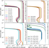 |
Fig. A.3 VMR profiles of CO and CH4 in our grid of disequilibrium chemistry models of WASP-107b. |
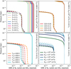 |
Fig. A.4 VMR profiles of N2 and NH3 in our grid of disequilibrium chemistry models of WASP-107b. |
Appendix B Corner plots of Cases 1 and 10
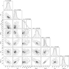 |
Fig. B.1 Corner plot for Case 1. |
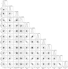 |
Fig. B.2 Corner plot for Case 10. |
Appendix C Best-fit spectra of Cases 15, 16, and 17
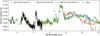 |
Fig. C.1 Best-fit spectra for Cases 15, 16, and 17 in which silicate condensates were fitted to the observations. |
Appendix D Tabulated retrieval outcomes
Summary of the retrievals with grey clouds with the nominal model (Case 1) listed first.
Summary of the retrievals with non-grey ‘Gaussian’ clouds with the nominal model (Case 10) listed first.
Summary of the retrievals with non-grey silicate clouds.
Summary of the retrievals with a slightly cooler grid (rst = 0.5) of forward models compared to the previous models presented in this study.
References
- Ackerman, A. S., & Marley, M. S., 2001, ApJ, 556, 872 [Google Scholar]
- Agúndez, M., 2025, A&A, 699, A306 [NASA ADS] [CrossRef] [EDP Sciences] [Google Scholar]
- Allard, F., Allard, N. F., Homeier, D., et al. 2007a, A&A, 474, L21 [NASA ADS] [CrossRef] [EDP Sciences] [Google Scholar]
- Allard, N. F., Kielkopf, J. F., & Allard, F. 2007b, Eur. Phys. J. D, 44, 507 [NASA ADS] [CrossRef] [Google Scholar]
- Allard, N. F., Spiegelman, F., & Kielkopf, J. F., 2016, A&A, 589, A21 [NASA ADS] [CrossRef] [EDP Sciences] [Google Scholar]
- Allard, N. F., Spiegelman, F., Leininger, T., & Molliere, P., 2019, A&A, 628, A120 [NASA ADS] [CrossRef] [EDP Sciences] [Google Scholar]
- Anderson, D. R., Collier Cameron, A., Delrez, L., et al. 2017, A&A, 604, A110 [NASA ADS] [CrossRef] [EDP Sciences] [Google Scholar]
- Asplund, M., Grevesse, N., Sauval, A. J., & Scott, P., 2009, ARA&A, 47, 481 [NASA ADS] [CrossRef] [Google Scholar]
- Azzam, A. A. A., Tennyson, J., Yurchenko, S. N., & Naumenko, O. V., 2016, MNRAS, 460, 4063 [NASA ADS] [CrossRef] [Google Scholar]
- Baeyens, R., Decin, L., Carone, L., et al. 2021, MNRAS, 505, 5603 [NASA ADS] [CrossRef] [Google Scholar]
- Baeyens, R., Konings, T., Venot, O., Carone, L., & Decin, L., 2022, MNRAS, 512, 4877 [NASA ADS] [CrossRef] [Google Scholar]
- Baeyens, R., Désert, J.-M., Petrignani, A., Carone, L., & Schneider, A. D. 2024, A&A, 686, A24 [NASA ADS] [CrossRef] [EDP Sciences] [Google Scholar]
- Barber, R. J., Strange, J. K., Hill, C., et al. 2014, MNRAS, 437, 1828 [CrossRef] [Google Scholar]
- Bard, A., & Kock, M., 1994, A&A, 282, 1014 [NASA ADS] [Google Scholar]
- Bard, A., Kock, A., & Kock, M., 1991, A&A, 248, 315 [NASA ADS] [Google Scholar]
- Barton, E. J., Yurchenko, S. N., & Tennyson, J., 2013, MNRAS, 434, 1469 [NASA ADS] [CrossRef] [Google Scholar]
- Barton, E. J., Hill, C., Czurylo, M., et al. 2017, J. Quant. Spec. Radiat. Transf., 203, 490 [CrossRef] [Google Scholar]
- Beatty, T. G., Welbanks, L., Schlawin, E., et al. 2024, ApJ, 970, L10 [Google Scholar]
- Bell, T. J., Welbanks, L., Schlawin, E., et al. 2023, Nature, 623, 709 [Google Scholar]
- Bell, T. J., Crouzet, N., Cubillos, P. E., et al. 2024, Nat. Astron., 8, 879 [Google Scholar]
- Benneke, B., & Seager, S., 2012, ApJ, 753, 100 [NASA ADS] [CrossRef] [Google Scholar]
- Bittner, D. M., & Bernath, P. F., 2018, ApJS, 236, 46 [Google Scholar]
- Borysow, A., 2002, A&A, 390, 779 [NASA ADS] [CrossRef] [EDP Sciences] [Google Scholar]
- Borysow, A., & Frommhold, L., 1989, ApJ, 341, 549 [NASA ADS] [CrossRef] [Google Scholar]
- Borysow, J., Frommhold, L., & Birnbaum, G., 1988, ApJ, 326, 509 [NASA ADS] [CrossRef] [Google Scholar]
- Borysow, A., Frommhold, L., & Moraldi, M., 1989, ApJ, 336, 495 [NASA ADS] [CrossRef] [Google Scholar]
- Borysow, A., Jorgensen, U. G., & Fu, Y., 2001, J. Quant. Spec. Radiat. Transf., 68, 235 [NASA ADS] [CrossRef] [Google Scholar]
- Buchner, J., 2021, J. Open Source Softw., 6, 3001 [CrossRef] [Google Scholar]
- Burrows, A., Ram, R. S., Bernath, P., Sharp, C. M., & Milsom, J. A., 2002, ApJ, 577, 986 [NASA ADS] [CrossRef] [Google Scholar]
- Caldas, A., Leconte, J., Selsis, F., et al. 2019, A&A, 623, A161 [NASA ADS] [CrossRef] [EDP Sciences] [Google Scholar]
- Carter, A. L., May, E. M., Espinoza, N., et al. 2024, Nat. Astron., 8, 1008 [Google Scholar]
- Chan, Y. M., & Dalgarno, A., 1965, Proc. Phys. Soc., 85, 227 [NASA ADS] [CrossRef] [Google Scholar]
- Chubb, K. L., Rocchetto, M., Yurchenko, S. N., et al. 2021, A&A, 646, A21 [NASA ADS] [CrossRef] [EDP Sciences] [Google Scholar]
- Coles, P. A., Yurchenko, S. N., & Tennyson, J., 2019, MNRAS, 490, 4638 [CrossRef] [Google Scholar]
- Coppola, C. M., Lodi, L., & Tennyson, J., 2011, MNRAS, 415, 487 [NASA ADS] [CrossRef] [Google Scholar]
- Dalgarno, A., & Williams, D. A., 1962, ApJ, 136, 690 [NASA ADS] [CrossRef] [Google Scholar]
- de Gruijter, W., Tsai, S.-M., Min, M., et al. 2025, A&A, 693, A132 [NASA ADS] [CrossRef] [EDP Sciences] [Google Scholar]
- Dijkstra, E., 1959, Numer. Math., 269 [Google Scholar]
- Drummond, B., Tremblin, P., Baraffe, I., et al. 2016, A&A, 594, A69 [NASA ADS] [CrossRef] [EDP Sciences] [Google Scholar]
- Drummond, B., Mayne, N. J., Baraffe, I., et al. 2018, A&A, 612, A105 [NASA ADS] [CrossRef] [EDP Sciences] [Google Scholar]
- Dulick, M., Bauschlicher,Jr., C. W., Burrows, A., et al. 2003, ApJ, 594, 651 [NASA ADS] [CrossRef] [Google Scholar]
- Dyrek, A., Min, M., Decin, L., et al. 2024, Nature, 625, 51 [Google Scholar]
- Edwards, B., Changeat, Q., Tsiaras, A., et al. 2023, ApJS, 269, 31 [NASA ADS] [CrossRef] [Google Scholar]
- Espinoza, N., Fortney, J. J., Miguel, Y., Thorngren, D., & Murray-Clay, R., 2017, ApJ, 838, L9 [Google Scholar]
- Falco, A., Zingales, T., Pluriel, W., & Leconte, J., 2022, A&A, 658, A41 [NASA ADS] [CrossRef] [EDP Sciences] [Google Scholar]
- Fisher, C., & Heng, K., 2018, MNRAS, 481, 4698 [Google Scholar]
- Fortney, J. J., Visscher, C., Marley, M. S., et al. 2020, AJ, 160, 288 [NASA ADS] [CrossRef] [Google Scholar]
- France, K., Loyd, R. O. P., Youngblood, A., et al. 2016, ApJ, 820, 89 [NASA ADS] [CrossRef] [Google Scholar]
- Fu, G., Welbanks, L., Deming, D., et al. 2024, Nature, 632, 752 [Google Scholar]
- Fuhr, J. R., Martin, G. A., & Wiese, W. L., 1988, J. Phys. Chem. Ref. Data, 17 [Google Scholar]
- GharibNezhad, E., Shayesteh, A., & Bernath, P. F., 2013, MNRAS, 432, 2043 [NASA ADS] [CrossRef] [Google Scholar]
- Gharib-Nezhad, E., Iyer, A. R., Line, M. R., et al. 2021, ApJS, 254, 34 [NASA ADS] [CrossRef] [Google Scholar]
- Gordon, I. E., Rothman, L. S., Hill, C., et al. 2017, J. Quant. Spec. Radiat. Transf., 203, 3 [NASA ADS] [CrossRef] [Google Scholar]
- Gordon, I. E., Rothman, L. S., Hargreaves, R. J., et al. 2022, J. Quant. Spec. Radiat. Transf., 277, 107949 [NASA ADS] [CrossRef] [Google Scholar]
- Griffith, C. A., 2014, Philos. Trans. Roy. Soc. Lond. Ser. A, 372, 20130086 [NASA ADS] [Google Scholar]
- Hargreaves, R. J., Hinkle, K. H., Bauschlicher,Jr., C. W., et al. 2010, AJ, 140, 919 [NASA ADS] [CrossRef] [Google Scholar]
- Harris, G. J., Tennyson, J., Kaminsky, B. M., Pavlenko, Y. V., & Jones, H. R. A., 2006, MNRAS, 367, 400 [Google Scholar]
- Helling, C., 2019, Annu. Rev. Earth Planet. Sci., 47, 583 [CrossRef] [Google Scholar]
- Heng, K., & Kitzmann, D., 2017, MNRAS, 470, 2972 [Google Scholar]
- Hobbs, R., Rimmer, P. B., Shorttle, O., & Madhusudhan, N., 2021, MNRAS, 506, 3186 [NASA ADS] [CrossRef] [Google Scholar]
- Hu, R., 2021, ApJ, 921, 27 [NASA ADS] [CrossRef] [Google Scholar]
- Huang, X., Gamache, R. R., Freedman, R. S., Schwenke, D. W., & Lee, T. J., 2014, J. Quant. Spectrosc. Radiative Transfer, 147, 134 [Google Scholar]
- Kiefer, S., Lecoq-Molinos, H., Helling, C., Bangera, N., & Decin, L., 2024, A&A, 682, A150 [NASA ADS] [CrossRef] [EDP Sciences] [Google Scholar]
- Konings, T., Baeyens, R., & Decin, L., 2022, A&A, 667, A15 [NASA ADS] [CrossRef] [EDP Sciences] [Google Scholar]
- Kreidberg, L., Line, M. R., Thorngren, D., Morley, C. V., & Stevenson, K. B., 2018, ApJ, 858, L6 [Google Scholar]
- Kurucz, R. L., 1992, Rev. Mexicana Astron. Astrofis., 23, 45 [Google Scholar]
- Kurucz, R. L., 1993, SYNTHE spectrum synthesis programs and line data [Google Scholar]
- Leconte, J., Chabrier, G., Baraffe, I., & Levrard, B., 2010, A&A, 516, A64 [NASA ADS] [CrossRef] [EDP Sciences] [Google Scholar]
- Lee, E. K. H., Tan, X., & Tsai, S.-M., 2024, MNRAS, 529, 2686 [NASA ADS] [CrossRef] [Google Scholar]
- Lee, E. K. H., Wardenier, J. P., Prinoth, B., et al. 2022, ApJ, 929, 180 [NASA ADS] [CrossRef] [Google Scholar]
- Li, G., Gordon, I. E., Rothman, L. S., et al. 2015, ApJS, 216, 15 [NASA ADS] [CrossRef] [Google Scholar]
- Line, M. R., & Parmentier, V., 2016, ApJ, 820, 78 [Google Scholar]
- Line, M. R., Liang, M. C., & Yung, Y. L., 2010, ApJ, 717, 496 [NASA ADS] [CrossRef] [Google Scholar]
- Lodders, K., 2010, in Astrophysics and Space Science Proceedings, 16, Principles and Perspectives in Cosmochemistry, 379 [Google Scholar]
- Lodders, K., & Fegley, B., 2002, Icarus, 155, 393 [Google Scholar]
- Lodders, K., & Fegley,Jr., B. 1999, in IAU Symposium, 191, Asymptotic Giant Branch Stars, eds. T. Le Bertre, A. Lebre, & C. Waelkens, 279 [Google Scholar]
- Loyd, R. O. P., France, K., Youngblood, A., et al. 2016, ApJ, 824, 102 [NASA ADS] [CrossRef] [Google Scholar]
- Lupu, R., Freedman, R., Gharib-Nezhad, E., Visscher, C., & Molliere, P., 2023, https://doi.org/10.5281/zenodo.7542068 [Google Scholar]
- MacDonald, R. J., Goyal, J. M., & Lewis, N. K., 2020, ApJ, 893, L43 [NASA ADS] [CrossRef] [Google Scholar]
- Madhusudhan, N., 2018, in Handbook of Exoplanets, eds. H. J. Deeg, & J. A. Belmonte, 104 [Google Scholar]
- Madhusudhan, N., Agúndez, M., Moses, J. I., & Hu, Y., 2016, Space Sci. Rev., 205, 285 [Google Scholar]
- Mahapatra, G., Helling, C., & Miguel, Y., 2017, MNRAS, 472, 447 [NASA ADS] [CrossRef] [Google Scholar]
- Marley, M. S., Ackerman, A. S., Cuzzi, J. N., & Kitzmann, D., 2013, in Comparative Climatology of Terrestrial Planets, eds. S. J. Mackwell, A. A. Simon-Miller, J. W. Harder, & M. A. Bullock, 367 [Google Scholar]
- Marley, M. S., Saumon, D., Visscher, C., et al. 2021, ApJ, 920, 85 [NASA ADS] [CrossRef] [Google Scholar]
- McKemmish, L. K., Masseron, T., Hoeijmakers, H. J., et al. 2019, MNRAS, 488, 2836 [Google Scholar]
- Millholland, S., Petigura, E., & Batygin, K., 2020, ApJ, 897, 7 [NASA ADS] [CrossRef] [Google Scholar]
- Min, M., Hovenier, J. W., & de Koter, A., 2005, A&A, 432, 909 [NASA ADS] [CrossRef] [EDP Sciences] [Google Scholar]
- Mizus, I. I., Alijah, A., Zobov, N. F., et al. 2017, MNRAS, 468, 1717 [NASA ADS] [CrossRef] [Google Scholar]
- Molaverdikhani, K., Henning, T., & Mollière, P., 2020, ApJ, 899, 53 [CrossRef] [Google Scholar]
- Mollière, P., van Boekel, R., Dullemond, C., Henning, T., & Mordasini, C., 2015, ApJ, 813, 47 [Google Scholar]
- Mollière, P., Wardenier, J. P., van Boekel, R., et al. 2019, A&A, 627, A67 [Google Scholar]
- Mordasini, C., van Boekel, R., Mollière, P., Henning, T., & Benneke, B., 2016, ApJ, 832, 41 [Google Scholar]
- Moses, J. I., 2014, Philos. Trans. Roy. Soc. Lond. Ser. A, 372, 20130073 [Google Scholar]
- Moses, J. I., Visscher, C., Fortney, J. J., et al. 2011, ApJ, 737, 15 [Google Scholar]
- Mukherjee, S., Batalha, N. E., Fortney, J. J., & Marley, M. S., 2023, ApJ, 942, 71 [NASA ADS] [CrossRef] [Google Scholar]
- Murphy, M. M., Beatty, T. G., Schlawin, E., et al. 2024, Nat. Astron., 8, 1562 [NASA ADS] [CrossRef] [Google Scholar]
- Nixon, M. C., & Madhusudhan, N., 2022, ApJ, 935, 73 [NASA ADS] [CrossRef] [Google Scholar]
- Novais, A., Fisher, C., Ghezzi, L., et al. 2025, MNRAS, 538, 2521 [Google Scholar]
- Öberg, K. I., Murray-Clay, R., & Bergin, E. A., 2011, ApJ, 743, L16 [Google Scholar]
- O’Brian, T. R., Wickliffe, M. E., Lawler, J. E., Whaling, W., & Brault, J. W., 1991, J. Opt. Soc. Am. B Opt. Phys., 8, 1185 [Google Scholar]
- Piaulet, C., Benneke, B., Rubenzahl, R. A., et al. 2021, AJ, 161, 70 [NASA ADS] [CrossRef] [Google Scholar]
- Pine, A. S., 1992, J. Chem. Phys., 97, 773 [Google Scholar]
- Pluriel, W., Leconte, J., Parmentier, V., et al. 2022, A&A, 658, A42 [NASA ADS] [CrossRef] [EDP Sciences] [Google Scholar]
- Polman, J., Waters, L. B. F. M., Min, M., Miguel, Y., & Khorshid, N., 2023, A&A, 670, A161 [NASA ADS] [CrossRef] [EDP Sciences] [Google Scholar]
- Polyansky, O. L., Kyuberis, A. A., Zobov, N. F., et al. 2018, MNRAS, 480, 2597 [NASA ADS] [CrossRef] [Google Scholar]
- Richard, C., Gordon, I. E., Rothman, L. S., et al. 2012, J. Quant. Spec. Radiat. Transf., 113, 1276 [NASA ADS] [CrossRef] [Google Scholar]
- Rothman, L. S., Gordon, I. E., Barber, R. J., et al. 2010, J. Quant. Spec. Radiat. Transf., 111, 2139 [NASA ADS] [CrossRef] [Google Scholar]
- Rothman, L. S., Gordon, I. E., Babikov, Y., et al. 2013, J. Quant. Spec. Radiat. Transf., 130, 4 [NASA ADS] [CrossRef] [Google Scholar]
- Ryabchikova, T., Piskunov, N., Kurucz, R. L., et al. 2015, Phys. Scr, 90, 054005 [Google Scholar]
- Sarkis, P., Mordasini, C., Henning, T., Marleau, G. D., & Mollière, P., 2021, A&A, 645, A79 [NASA ADS] [CrossRef] [EDP Sciences] [Google Scholar]
- Sing, D. K., Rustamkulov, Z., Thorngren, D. P., et al. 2024, Nature, 630, 831 [NASA ADS] [CrossRef] [Google Scholar]
- Sousa-Silva, C., Hesketh, N., Yurchenko, S. N., Hill, C., & Tennyson, J., 2014, J. Quant. Spec. Radiat. Transf., 142, 66 [Google Scholar]
- Sánchez-Lavega, A., Irwin, P., & García Muñoz, A. 2023, A&AR, 31, 5 [Google Scholar]
- Thorngren, D., & Fortney, J. J., 2019, ApJ, 874, L31 [Google Scholar]
- Thorngren, D., Gao, P., & Fortney, J. J., 2019, ApJ, 884, L6 [Google Scholar]
- Tsai, S.-M., Lyons, J. R., Grosheintz, L., et al. 2017, ApJS, 228, 20 [NASA ADS] [CrossRef] [Google Scholar]
- Tsai, S.-M., Kitzmann, D., Lyons, J. R., et al. 2018, ApJ, 862, 31 [NASA ADS] [CrossRef] [Google Scholar]
- Tsai, S.-M., Malik, M., Kitzmann, D., et al. 2021, ApJ, 923, 264 [NASA ADS] [CrossRef] [Google Scholar]
- Tsai, S.-M., Lee, E. K. H., Powell, D., et al. 2023, Nature, 617, 483 [CrossRef] [Google Scholar]
- Tsantaki, M., Sousa, S. G., Adibekyan, V. Z., et al. 2013, A&A, 555, A150 [NASA ADS] [CrossRef] [EDP Sciences] [Google Scholar]
- Underwood, D. S., Tennyson, J., Yurchenko, S. N., et al. 2016, MNRAS, 459, 3890 [NASA ADS] [CrossRef] [Google Scholar]
- Venot, O., Hébrard, E., Agúndez, M., et al. 2012, A&A, 546, A43 [NASA ADS] [CrossRef] [EDP Sciences] [Google Scholar]
- Venot, O., Cavalié, T., Bounaceur, R., et al. 2020, A&A, 634, A78 [NASA ADS] [CrossRef] [EDP Sciences] [Google Scholar]
- Visscher, C., Lodders, K., & Fegley,Jr., B. 2010, ApJ, 716, 1060 [NASA ADS] [CrossRef] [Google Scholar]
- Welbanks, L., Bell, T. J., Beatty, T. G., et al. 2024, Nature, 630, 836 [NASA ADS] [CrossRef] [Google Scholar]
- Welbanks, L., & Madhusudhan, N., 2019, AJ, 157, 206 [NASA ADS] [CrossRef] [Google Scholar]
- Wenger, C., & Champion, J. P., 1998, J. Quant. Spec. Radiat. Transf., 59, 471 [Google Scholar]
- Wilzewski, J. S., Gordon, I. E., Kochanov, R. V., Hill, C., & Rothman, L. S., 2016, J. Quant. Spec. Radiat. Transf., 168, 193 [NASA ADS] [CrossRef] [Google Scholar]
- Yadin, B., Veness, T., Conti, P., et al. 2012, MNRAS, 425, 34 [NASA ADS] [CrossRef] [Google Scholar]
- Yip, K. H., Changeat, Q., Nikolaou, N., et al. 2021, AJ, 162, 195 [NASA ADS] [CrossRef] [Google Scholar]
- Youngblood, A., France, K., Loyd, R. O. P., et al. 2016, ApJ, 824, 101 [Google Scholar]
- Yu, H., & Dai, F., 2024, ApJ, 972, 159 [Google Scholar]
- Yurchenko, S. N., & Tennyson, J., 2014, MNRAS, 440, 1649 [Google Scholar]
- Yurchenko, S. N., Barber, R. J., & Tennyson, J., 2011, MNRAS, 413, 1828 [Google Scholar]
- Yurchenko, S. N., Tennyson, J., Barber, R. J., & Thiel, W., 2013, J. Mol. Spectrosc., 291, 69 [Google Scholar]
- Yurchenko, S. N., Amundsen, D. S., Tennyson, J., & Waldmann, I. P., 2017, A&A, 605, A95 [NASA ADS] [CrossRef] [EDP Sciences] [Google Scholar]
- Yurchenko, S. N., Mellor, T. M., Freedman, R. S., & Tennyson, J., 2020, MNRAS, 496, 5282 [NASA ADS] [CrossRef] [Google Scholar]
- Zahnle, K. J., & Marley, M. S., 2014, ApJ, 797, 41 [CrossRef] [Google Scholar]
- Zhang, X., 2020, Res. Astron. Astrophys., 20, 099 [NASA ADS] [CrossRef] [Google Scholar]
All Tables
Dominant reactions that convert OH into SO2 for different metallicities and pressure levels.
Summary of the retrievals with grey clouds with the nominal model (Case 1) listed first.
Summary of the retrievals with non-grey ‘Gaussian’ clouds with the nominal model (Case 10) listed first.
Summary of the retrievals with a slightly cooler grid (rst = 0.5) of forward models compared to the previous models presented in this study.
All Figures
|
Fig. 1 Selection of the 180 computed PT profiles with PICASO for C/O=0.46. The line transparency corresponds to intrinsic temperature, from a full line for Tint=100 K to almost transparent for Tint=500 K. The shaded grey region indicates layers where the radiative-convective boundaries are located in all 180 PT profiles. |
| In the text | |
|
Fig. 2 VMR profiles of key species CH4, SO2, and NH3 in our grid of disequilibrium chemistry models of WASP-107b. Chemical equilibrium is plotted with thin, dashed lines. The nominal model of Z=10Z⊙, C/O=0.46, Tint=400 K, and log Kzz=9(cm2/s) was chosen to be in agreement with previous studies (Dyrek et al. 2024; Welbanks et al. 2024). |
| In the text | |
|
Fig. 3 Dominant reactions (by fastest reaction rate) that involve SO and SO2, for three different combinations of metallicity and eddy diffusion coefficient. Forward rates are shown by solid lines; backward rates by dotted lines. The other values of these simulations are Tint=400 K and C/O=0.46. |
| In the text | |
|
Fig. 4 Dominant reactions (by fastest reaction rate) that produce/destroy S, for three different metallicities. Forward rates are shown by solid lines; backward rates by dotted lines. The other values of the simulations are Tint=400 K, C/O=0.46 and log Kzz=9(cm2/s). |
| In the text | |
|
Fig. 5 VMR of SO2 and dominant H-producing reactions for a nominal model (Z=10 Z⊙, C/O=0.46, Tint=400 K, log Kzz=9 cm2/s) that includes all available photodissociation cross-sections (upper left panel), and three limiting cases where only the photolysis of one particular source is considered (N2, H2O., or NH3), copying the experiment of Dyrek et al. (2024). Panels that show thermochemical reaction rates show both their forward (solid lines) and backward (dashed) rates. |
| In the text | |
|
Fig. 6 Quenching VMR (left panel) and estimated quenching pressure (right panel) of CH4 versus intrinsic temperature Tint for various eddy diffusion coefficients in low (Z=1 Z⊙) and high (Z=10 Z⊙) metallicity atmospheres. The models with log Kzz = 6 (cgs) are not included as not all atmospheres are quenched at such weak vertical mixing. |
| In the text | |
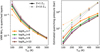 |
Fig. 7 Same as Fig. 6, now for NH3. |
| In the text | |
|
Fig. 8 Cloud-free synthetic spectra of our grid of 1D-RCPE models for WASP-107b computed with petitRADTRANS. The top row indicates the dominant opacity sources, with secondary contributors in brackets. |
| In the text | |
|
Fig. 9 Best-fit spectrum of Case 1 with molecular contributions (upper panel). The bottom panels show spectra within 1σ, 2σ, and 3σ uncertainty levels of the mean posterior values. The data plotted in the upper panel consists of HST WFC3 (Kreidberg et al. 2018) and JWST NIRCam (Welbanks et al. 2024). |
| In the text | |
|
Fig. 10 Best-fit spectrum for Case 10. The data plotted in the bottom panel consists of HST WFC3 (Kreidberg et al. 2018), JWST NIRCam (Welbanks et al. 2024), and JWST MIRI/LRS (Dyrek et al. 2024). |
| In the text | |
|
Fig. 11 Best-fit PT profile (upper left), VMRs of key species (upper right), and model spectra (bottom) of retrievals Case 19 and Case 10 that have Gaussian clouds and a free wavelength-dependent opacity slope. The grid of models used for Case 19 are approximately 100 K cooler in the isothermal layers (rst=0.5) compared to those used for Case 10(rst = 1). Note that both retrievals converge to a different set of grid parameters (Z, C/O, Tint, Kzz), which affects the VMRs and PT profiles, but a fit of similar quality can be achieved. |
| In the text | |
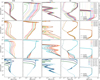 |
Fig. A.1 Same as Fig. 2 for HCN, CO2, C2H2, SO, and H2S. |
| In the text | |
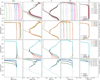 |
Fig. A.2 Same as Fig. 2 for H2O, OH, H, CO, and H2. |
| In the text | |
|
Fig. A.3 VMR profiles of CO and CH4 in our grid of disequilibrium chemistry models of WASP-107b. |
| In the text | |
|
Fig. A.4 VMR profiles of N2 and NH3 in our grid of disequilibrium chemistry models of WASP-107b. |
| In the text | |
|
Fig. B.1 Corner plot for Case 1. |
| In the text | |
|
Fig. B.2 Corner plot for Case 10. |
| In the text | |
|
Fig. C.1 Best-fit spectra for Cases 15, 16, and 17 in which silicate condensates were fitted to the observations. |
| In the text | |
Current usage metrics show cumulative count of Article Views (full-text article views including HTML views, PDF and ePub downloads, according to the available data) and Abstracts Views on Vision4Press platform.
Data correspond to usage on the plateform after 2015. The current usage metrics is available 48-96 hours after online publication and is updated daily on week days.
Initial download of the metrics may take a while.