| Issue |
A&A
Volume 701, September 2025
|
|
|---|---|---|
| Article Number | A264 | |
| Number of page(s) | 10 | |
| Section | Planets, planetary systems, and small bodies | |
| DOI | https://doi.org/10.1051/0004-6361/202555471 | |
| Published online | 24 September 2025 | |
Magnetohydrodynamic simulations preliminarily predict the habitability and radio emission of TRAPPIST-1e
1
Department of Earth and Space Sciences, Southern University of Science and Technology,
Shenzhen
518055,
PR
China
2
Institute for Fusion Studies, University of Texas,
Austin,
TX
78712,
USA
3
State Key Laboratory of Multiphase Flow in Power Engineering, Xi’an Jiaotong University,
Xi’an
710049,
PR
China
★ Corresponding author: This email address is being protected from spambots. You need JavaScript enabled to view it.
Received:
10
May
2025
Accepted:
5
August
2025
Abstract
Context. TRAPPIST-1e, an Earth-sized exoplanet in the habitable zone of the nearby M dwarf TRAPPIST-1, may experience magnetospheric responses that vary with stellar space weather, which could potentially influence both its habitability and radio emissions.
Aims. Our objective is to investigate how different Earth-like magnetospheric configurations of TRAPPIST-1e – specifically variations in dipolar magnetic field strength and axial tilt – respond to diverse stellar space weather conditions, including events analogous to coronal mass ejections (CMEs), and to assess their implications for potential habitability and expected radio emissions.
Methods. We conducted 3D magnetohydrodynamic simulations of the TRAPPIST-1e system using the PLUTO code in spherical coordinates. The planetary magnetic field was modelled as dipolar, with equatorial strengths from Earth-like to several times stronger. The dipole axis spans a representative range of axial tilts. We investigate four stellar wind environments, from sub-Alfvénic flow to CME-like disturbances. Planetary shielding was quantified based on the magnetopause standoff distance, and radio powers were estimated via empirical scaling laws.
Results. Our simulations show that both shielding and radio power depend strongly on the magnetic configuration. Stronger fields increase protection, while larger tilts reduce it. Radio power increases with both field strength and tilt across all wind regimes. An Earth-like magnetic field can provide effective shielding even under intense CMEs, whereas high tilts require stronger fields. Predicted radio powers reach ~1020 erg s−1 during CMEs, making bursts from close-in, magnetised planets more detectable. However, for TRAPPIST-1e, the maximum cyclotron frequency lies below the Earth’s ionospheric cutoff (~10 MHz), making ground-based detection currently infeasible.
Key words: Sun: magnetic fields / planets and satellites: terrestrial planets / planet-star interactions
© The Authors 2025
 Open Access article, published by EDP Sciences, under the terms of the Creative Commons Attribution License (https://creativecommons.org/licenses/by/4.0), which permits unrestricted use, distribution, and reproduction in any medium, provided the original work is properly cited.
This article is published in open access under the Subscribe to Open model. This email address is being protected from spambots. You need JavaScript enabled to view it. to support open access publication.
1 Introduction
M-dwarf stars are the most abundant stellar population in the Universe and constitute the vast majority of stars within our galaxy and beyond. Their ubiquity and intrinsic characteristics – particularly their low masses, low luminosities, and relatively small sizes – make them compelling targets in the search for potentially habitable exoplanets. Due to their low luminosities, M dwarfs possess habitable zones located much closer to them compared to solar-type stars. As a result, planets within these zones are likely tidally locked, which may inhibit their internal dynamo processes and reduce or suppress the generation of a strong intrinsic magnetic field. Moreover, the exceptionally long lifespans of M dwarfs, often spanning billions to tens of billions of years, provide ample temporal windows conducive to the emergence and evolution of life.
Planets situated within the habitable zones of M dwarfs may maintain surface temperatures compatible with the presence of liquid water, a fundamental prerequisite for life as we understand it. However, the habitability of these planets is significantly influenced by the host stars’ magnetic activity. Young M dwarfs frequently exhibit intense stellar winds and high levels of X-ray and ultraviolet radiation, which can profoundly affect planetary atmospheres. In this context, a planetary magnetic field plays a potentially critical protective role by altering the interaction between the stellar wind and the atmosphere. However, recent studies suggest that magnetisation alone is not sufficient to prevent atmospheric loss, as significant escape can still occur along open field lines at the polar caps and cusps (Gunell et al. 2018). Thus, while strong magnetospheres can mitigate some erosion mechanisms, they do not universally suppress atmospheric escape, and habitability must be evaluated in a broader physical context.
Furthermore, given their close orbital proximity, planets around M dwarfs can exist within the stellar Alfvén surface, a condition conducive to electromagnetic star–planet interactions (SPIs). Within this sub-Alfvénic regime, planets can interact magnetically with their host stars, forming Alfvén wings – structures capable of carrying substantial energy fluxes. This process is analogous to the well-studied interaction between Jupiter and its moon Io within our Solar System. Theoretical models such as the ‘unipolar inductor’ model proposed by Goldreich & Lynden-Bell (1969) and the Alfvén wings model developed by Neubauer (1980) and Goertz (1980) have provided foundational frameworks for interpreting such interactions.
Given the substantial differences in stellar properties between M dwarfs and the Sun – including age, metallicity, magnetic field strength, and rotation rates – the direct application of Solar System-based space weather models to exoplanetary systems remains problematic. If stellar wind conditions (dynamic and magnetic pressures) are intense, planetary habitability becomes heavily dependent on the intrinsic planetary magnetic field strength. A robust intrinsic magnetic field can effectively prevent atmospheric stripping by stellar winds, protecting the volatile constituents crucial for habitability. Conversely, weak magnetic fields might allow substantial atmospheric loss, diminishing a planet’s potential for sustaining life (Jakosky et al. 2015; Airapetian et al. 2020).
The detection of radio emissions emanating from planetary magnetospheres provides a powerful method for probing these magnetic fields (Hess & Zarka 2011). However, with current observational capabilities, no detected radio signals have been attributed to either intrinsic planetary magnetospheres or SPIs. Recent observations, including those of Proxima Centauri (Pérez-Torres et al. 2021), Tau Boötis (Turner et al. 2021), and YZ Ceti (Pineda & Villadsen 2023; Trigilio et al. 2023), have provided intriguing yet inconclusive evidence.
In particular, the TRAPPIST-1 system offers a significant opportunity to explore these phenomena due to its unique configuration of multiple Earth-sized planets orbiting within or near the habitable zone of a very low-mass M 8 star (Gillon et al. 2016, 2017). TRAPPIST-1e, which is located within its star’s habitable zone, serves as an ideal candidate for investigating habitability conditions and radio emission scenarios driven by SPIs. Observations of TRAPPIST-1 have suggested active stellar coronae and chromospheres (Bourrier et al. 2017; Wheatley et al. 2017). Variations in stellar wind conditions and Alfvén surface locations predicted by different models (Garraffo et al. 2017; Dong et al. 2018) further emphasise the complexity of assessing habitability in this system.
Recent studies indicate significant variability in expected radio emissions depending on planetary orbital positions relative to the stellar Alfvén surface, highlighting potential SPIdriven processes in the TRAPPIST-1 system (Réville et al. 2024; Pérez-Torres et al. 2021). TRAPPIST-1e, owing to its proximity and orbital characteristics, is particularly suited for detailed investigations of these interactions. Systematic studies of TRAPPIST-1e’s magnetic environment and its associated radio emissions provide critical insights into planetary magnetospheric configurations, star–planet electromagnetic interactions, and their implications for planetary habitability. Future radio observations of systems like TRAPPIST-1 hold promise for significantly advancing our capabilities to characterise exoplanetary magnetospheres and potentially detect signatures indicative of habitable conditions beyond the Solar System.
In this study, we investigated the magnetic response of the TRAPPIST-1e system under various terrestrial-like magnetic field strengths and different space weather conditions, including the impact of stellar winds on planetary habitability and associated radio emission. Our methodology closely follows previous studies dedicated to analysing how space weather affects exoplanetary habitability and planetary magnetospheric radio emissions (Varela et al. 2022a,b), including for the Proxima b planetary system (Peña-Moñino et al. 2024). The structure of the paper is as follows: in Sect. 2, we introduce the single-fluid magnetohydrodynamic (MHD) numerical model employed in our simulations. In Sect. 3, we analyse the effects of various space weather conditions on the habitability of TRAPPIST-1e. Section 4 presents calculations of predicted radio emissions under different scenarios. Finally, Sect. 5 summarises our findings and provides a discussion.
2 Numerical model of PLUTO
We employed the ideal MHD module of the open-source PLUTO code (Mignone et al. 2007) in spherical coordinates to model the time evolution of a single-fluid, fully ionised polytropic plasma under the non-resistive and inviscid approximation. The system of equations solved includes mass, momentum, magnetic induction, and total energy conservation, expressed in conservative form as
![Mathematical equation: $\[\frac{\partial \rho}{\partial t}+\nabla \cdot(\rho \mathbf{v})=0,\]$](/articles/aa/full_html/2025/09/aa55471-25/aa55471-25-eq1.png) (1)
(1)
![Mathematical equation: $\[\frac{\partial \mathbf{m}}{\partial t}+\nabla \cdot\left[\mathbf{m v}-\frac{\mathbf{B B}}{\mu_0}+\mathbf{I}\left(p+\frac{B^2}{2 \mu_0}\right)\right]^T=0,\]$](/articles/aa/full_html/2025/09/aa55471-25/aa55471-25-eq2.png) (2)
(2)
![Mathematical equation: $\[\frac{\partial \mathbf{B}}{\partial t}+\nabla \times \mathbf{E}=0,\]$](/articles/aa/full_html/2025/09/aa55471-25/aa55471-25-eq3.png) (3)
(3)
![Mathematical equation: $\[\frac{\partial E_t}{\partial t}+\nabla \cdot\left[\left(\frac{1}{2} \rho \mathbf{v}^2+\rho e+p\right) \mathbf{v}+\frac{\mathbf{E} \times \mathbf{B}}{\mu_0}\right]=0,\]$](/articles/aa/full_html/2025/09/aa55471-25/aa55471-25-eq4.png) (4)
(4)
where ρ is the mass density, v is the velocity field, m = ρv the momentum density, B the magnetic field, E = −(v × B) the electric field, p the thermal pressure and ![Mathematical equation: $\[E_{t}=\rho e+\frac{1}{2} \rho \mathbf{v}^{2}+\frac{\mathbf{B}^{2}}{2 \mu_{0}}\]$](/articles/aa/full_html/2025/09/aa55471-25/aa55471-25-eq5.png) the total energy density. The internal energy (ρe) is closed via the ideal gas equation of state:
the total energy density. The internal energy (ρe) is closed via the ideal gas equation of state:
![Mathematical equation: $\[\rho e=\frac{p}{\gamma-1},\]$](/articles/aa/full_html/2025/09/aa55471-25/aa55471-25-eq6.png) (5)
(5)
where γ = 5/3 is the adiabatic index.
For a fully ionised proton-electron plasma, we adopted a mean molecular weight μ = 1/2, so the number density is
![Mathematical equation: $\[n=\frac{\rho}{\mu m_p},\]$](/articles/aa/full_html/2025/09/aa55471-25/aa55471-25-eq7.png) (6)
(6)
and the pressure is
![Mathematical equation: $\[p=n k_B T,\]$](/articles/aa/full_html/2025/09/aa55471-25/aa55471-25-eq8.png) (7)
(7)
where kB is Boltzmann’s constant and T the temperature. The sound speed is defined as
![Mathematical equation: $\[c_s=\sqrt{\frac{\gamma p_t}{\rho}},\]$](/articles/aa/full_html/2025/09/aa55471-25/aa55471-25-eq9.png) (8)
(8)
where pt is the thermal pressure of the single-fluid plasma.
The equations were integrated using a Harten–Lax–van Leer approximate Riemann solver with a diffusive minmod limiter. The magnetic field was initialised to be divergence-free and maintained as such throughout the simulations via a mixed hyperbolic or parabolic divergence-cleaning technique (Dedner et al. 2002).
2.1 Basic setting
The simulation domain is defined as a 3D spherical grid composed of 128 radial cells, 48 polar cells uniformly distributed in θ ∈ [0, π], and 96 azimuthal cells covering ϕ ∈ [0, 2π]. The computational domain consists of a concentric shell centred on TRAPPIST-1e, with the radial range extending from the inner boundary Rin = 2.0Re to the outer boundary Rout = 30Re, where Re = 0.918 R⊕ is the radius of TRAPPIST-1 e (Gillon et al. 2016). The radial grid spacing is uniform, and all simulations assume a characteristic stellar wind speed V = 107 cm/s.
An upper ionosphere model is implemented between Rin and R = 2.2 Re, prescribing plasma inflow driven by field-aligned currents (FACs). This region provides a critical boundary layer where electric fields influence plasma motion. To prevent artificial numerical reflections, the outer boundary is divided into an upstream region with fixed stellar wind parameters and a down-stream region with zero radial derivative conditions ∂/∂r = 0 for all variables.
The initial conditions are set with a cutoff point to the interplanetary magnetic field (IMF) at Rcut = 6 Re, which approximates the location where the planetary magnetic pressure dominates over the stellar wind. Although simulations are performed in spherical polar coordinates (r, θ, ϕ), some quantities are expressed in Cartesian coordinates for clarity in physical interpretation. In the spherical system, r is the radial distance from the planet centre, θ is the colatitude measured from the planetary magnetic dipole axis (north pole), and ϕ is the azimuthal angle. The Cartesian coordinate system (x, y, z) shares the same origin with the spherical system at the planetary centre. The z-axis is aligned with the planetary magnetic dipole axis, the x-axis points along the star-planet line (with the star at x < 0), and the y-axis completes the right-handed system. This coordinate framework is applied consistently throughout the analysis.
A density cavity is introduced in the dayside magnetosphere according to
![Mathematical equation: $\[x<R_{\mathrm{cut}}-\frac{y^2+z^2}{R_{\mathrm{cut}} * \sqrt{R_{\mathrm{cut}}}},\]$](/articles/aa/full_html/2025/09/aa55471-25/aa55471-25-eq10.png) (9)
(9)
with (x,y,z) are the Cartesian coordinates, where the plasma velocity is zero. To compute the local Alfvén speed, we used
![Mathematical equation: $\[v_A=\frac{B}{\sqrt{\mu_0 \rho}},\]$](/articles/aa/full_html/2025/09/aa55471-25/aa55471-25-eq11.png) (10)
(10)
with ρ = nswmp, where nsw is the stellar wind particle density.
The planetary magnetic field is modelled as a dipole, rotated by 90° in the YZ plane relative to the grid to avoid numerical singularities at the poles. The model assumes that the planet’s magnetic and rotation axes are aligned. Obliquity effects are introduced by adjusting the direction of the IMF and stellar wind vectors.
Although the simulation does not resolve microphysical plasma behaviour due to grid limitations, it successfully captures the primary magnetospheric structures such as the bow shock, magnetopause, and magnetosheath, similar to previous MHD studies (Varela et al. 2015, 2016a,b, 2018). Simulations are evolved until a steady state is reached, typically after τ = L/V ≈ 15 code units, equivalent to t ≈ 16 minutes of physical time. This timescale corresponds to the Alfvén crossing time over the domain, sufficient to resolve the steady response of the magnetosphere to constant space weather conditions. The transient response to evolving space weather, planetary rotation, and orbital motion are not included in this study and will be addressed in future work.
2.2 Upper ionosphere model
The upper ionospheric domain in our simulations is defined between radial distances of R = 2.0Re and R = 2.2Re, following the approach of Büchner et al. (2003). This region is critical for prescribing plasma inflow from FACs into the simulation domain. Below this boundary, the magnetic field intensity becomes too large, resulting in prohibitively small simulation time steps. Moreover, since the single-fluid MHD approximation fails to capture kinetic processes prominent in the inner ionosphere and plasmasphere, these inner regions are excluded from the simulation domain.
To compute the FACs, we began by evaluating the total current,
![Mathematical equation: $\[\mathbf{J}=\frac{1}{\mu_0} \nabla \times \mathbf{B},\]$](/articles/aa/full_html/2025/09/aa55471-25/aa55471-25-eq12.png) (11)
(11)
then extracted the perpendicular current component,
![Mathematical equation: $\[\mathbf{J}_{\perp}=\mathbf{J}-(\mathbf{J} \cdot \mathbf{B}) \frac{\mathbf{B}}{|\mathbf{B}|^2}.\]$](/articles/aa/full_html/2025/09/aa55471-25/aa55471-25-eq13.png) (12)
(12)
This then allowed us to find the FAC as
![Mathematical equation: $\[\mathbf{J}_{\mathrm{FAC}}=\mathbf{J}-\mathbf{J}_{\perp}.\]$](/articles/aa/full_html/2025/09/aa55471-25/aa55471-25-eq14.png) (13)
(13)
The electric field in the upper ionosphere is derived using an empirical Pedersen conductivity σ, defined as
![Mathematical equation: $\[\sigma=\frac{40 E_0 ~\sqrt{F_E}}{16+E_0^2},\]$](/articles/aa/full_html/2025/09/aa55471-25/aa55471-25-eq15.png) (14)
(14)
where E0 = kBTe is the mean electron energy in keV, and ![Mathematical equation: $\[F_{E}=n_{e} \sqrt{E_{0} /(2 \pi m_{e})}\]$](/articles/aa/full_html/2025/09/aa55471-25/aa55471-25-eq16.png) is the energy flux in erg/cm2 s (Büchner & Zelenyi 1987). We adopted a fixed electron temperature of Te = 104 K, which corresponds to a mean electron energy of E0 ≈ 8.6 × 10⁻⁴ keV. This energy is substituted into the empirical conductivity formula. The electron density ne is dynamically extracted from the simulation grid, resulting in a conductivity σ that varies both spatially and temporally across the simulation domain. The electric field is then
is the energy flux in erg/cm2 s (Büchner & Zelenyi 1987). We adopted a fixed electron temperature of Te = 104 K, which corresponds to a mean electron energy of E0 ≈ 8.6 × 10⁻⁴ keV. This energy is substituted into the empirical conductivity formula. The electron density ne is dynamically extracted from the simulation grid, resulting in a conductivity σ that varies both spatially and temporally across the simulation domain. The electric field is then
![Mathematical equation: $\[\mathbf{E}=\frac{\mathbf{J}_{\mathrm{FAC}}}{\sigma}.\]$](/articles/aa/full_html/2025/09/aa55471-25/aa55471-25-eq17.png) (15)
(15)
The plasma drift velocity in this region was calculated from the standard relation:
![Mathematical equation: $\[\mathbf{u}=\frac{\mathbf{E} \times \mathbf{B}}{|\mathbf{B}|^2}.\]$](/articles/aa/full_html/2025/09/aa55471-25/aa55471-25-eq18.png) (16)
(16)
To control the simulation time step, we imposed a fixed Alfvén speed (vA) by prescribing the density profile as
![Mathematical equation: $\[\rho=\frac{|\mathbf{B}|^2}{\mu_0 v_A^2},\]$](/articles/aa/full_html/2025/09/aa55471-25/aa55471-25-eq19.png) (17)
(17)
where vA is set ~104 km/s depending on the IMF strength and stellar wind density. This ensures numerical stability across different space weather configurations.
The pressure profile was initialised with a smooth transition to the simulation domain and defined in relation to the sound speed:
![Mathematical equation: $\[p=n \frac{1}{\gamma}\left[\left(c_p-c_{s w}\right) \frac{r^3-R_s^3}{R_{\mathrm{in}}^3-R_s^3}+c_{s w}\right]^2,\]$](/articles/aa/full_html/2025/09/aa55471-25/aa55471-25-eq20.png) (18)
(18)
where ![Mathematical equation: $\[\gamma=5 / 3, c_{p}=\sqrt{\gamma k_{B} T_{p} / m_{p}}, c_{s w}=\sqrt{\gamma k_{B} T_{s w} / m_{p}}, R_{S}\]$](/articles/aa/full_html/2025/09/aa55471-25/aa55471-25-eq21.png) is the outer boundary of the soft coupling region (in our simulations, we adopted Tp = 104 K) and represents the ionospheric plasma temperature, and Tsw is the stellar wind temperature. Adding the soft coupling region improves the description of the plasmas flows towards the planet surface, isolating the simulation domain from spurious numerical effects of the inner boundary conditions (Varela et al. 2016a,b,c).
is the outer boundary of the soft coupling region (in our simulations, we adopted Tp = 104 K) and represents the ionospheric plasma temperature, and Tsw is the stellar wind temperature. Adding the soft coupling region improves the description of the plasmas flows towards the planet surface, isolating the simulation domain from spurious numerical effects of the inner boundary conditions (Varela et al. 2016a,b,c).
During the early stages of the simulation, the pressure and density gradients generate plasma outflows from the upper ionosphere into the domain until a quasi-steady state is established. This process is driven by the balance between stellar wind injection and ionospheric outflow.
We benchmarked the model against the global magnetosphere configuration described by Samsonov et al. (2016). Using similar parameters (e.g. n = 5 cm−3, Vx = −400 km/s, T = 2 × 10⁵ K, By = −Bx = 3.5nT), the predicted magnetopause locations Rx = 10.7 Re, Ry = 16.8 Re, Rz = 14.9 Re show good agreement with their results. The computed electric fields near the bow shock and inside the magnetosheath are consistent with Cluster observations (de Keyser et al. 2005), except in cases with extreme IMF strength.
For a Carrington-like event (Ridley et al. 2006) with n = 750 cm−3, Vx = −1600 km/s, T = 3.5 × 10⁷ K, |B| = 200 nT, our model predicts Rmsd/Re ~ 1.22 by extrapolation, which matches within the expected limits. Finally, we find that the electric field structure in the upper ionosphere remains relatively unchanged due to the fixed density. Both the intensity and orientation of FACs are within the range of Earth-based observational and modelling results (from nA/m2 to several μA/m2 under varying space weather conditions; Weimer 2001; Waters et al. 2001; Ritter et al. 2013; Bunescu et al. 2019; Zhang et al. 2020).
3 The habitability of TRAPPIST-1e
Figure 1 presents a 3D schematic of the TRAPPIST-1e system, including the M dwarf TRAPPIST-1, the stellar wind (green streamlines), IMF (white streamlines), the planet TRAPPIST-1e (right), and its dipolar magnetic field lines (also white). The stellar wind is assumed to be radial, and the planetary magnetic axis is aligned such that the rotational axis of TRAPPIST-1e is perpendicular to the ecliptic (tilt = 0°). On the dayside, interaction between the stellar wind and the planetary magnetic field leads to the formation of a bow shock (BS), marked by plasma pileup and density enhancement in red. The stellar wind compresses the planetary field on the dayside and stretches it into a magnetotail on the nightside. Reconnection between the IMF and the planetary magnetic field occurs near the magnetopause, driving localised magnetic erosion and flux transport.
3.1 Parameter settings in the simulation
We explored a range of space weather scenarios classified into calm and extreme regimes. The calm regime includes three distinct sub-cases: (1) a sub-Alfvénic scenario with a stellar surface magnetic field of 1200 G and low wind dynamic pressure (MA < 1), (2) a transition scenario with reduced stellar magnetic field (600 G), and (3) a super-Alfvénic case where dynamic pressure dominates over magnetic pressure, forming a well-defined bow shock. The extreme space weather case simulates a coronal mass ejection (CME)-like event with enhanced wind velocity, density, and magnetic field, scaled from the super-Alfvénic case by factors of 2.5, 5, and 10, respectively, following (Peña-Moñino et al. 2024).
Table 1 summarises the simulation parameters for all scenarios. The transition scenario was recalculated according to the parameters of the sub-Alfvén region by reducing the magnetic field from 1200 to 600 G. All other space weather condition parameters were adjusted to the orbital environment of TRAPPIST-1e according to the parameter settings for Proxima b planets in Peña-Moñino et al. (2024, assuming that the TRAPPIST-1 stars have the same mass loss rate as Proxima Cen). In all cases, the IMF is assumed to be radial.
The planetary magnetic field was assumed to be dipolar with strengths of 0.32, 0.64, and 1.28 G (Earth-like to 4× Earth), and the stellar wind temperature was fixed at TSW = 2.6 × 10⁵ K. Simulations explored various tilt angles from 0° to 45° to evaluate the impact of magnetic obliquity on the magnetospheric response and radio emission.
Figure 2 presents meridional plane of the TRAPPIST-1e magnetosphere under four representative space weather conditions: sub-Alfvénic (Fig. 2a), transition (Fig. 2b), super-Alfvénic (Fig. 2c), and CME-like (Fig. 2d). In the sub-Alfvénic regime (MA < 1), which corresponds to a stellar magnetic field of 1200 G, the interaction is magnetically dominated, and no bow shock is formed. The transition case maintains similar stellar wind parameters but with a reduced stellar magnetic field (600 G), leading to lower external magnetic pressure. This allows the planetary magnetic field to better resist stellar wind intrusion, resulting in a more expanded magnetosphere. A weak bow shock begins to form near the planetary nose. Hemispheric density asymmetry is a general feature across all simulated cases. However, in the transition case, the asymmetry appears more pronounced than sub-Alfvénic, with enhanced plasma compression and accumulation in the southern hemisphere – likely resulting from the combined influence of the magnetospheric topology and the orientation of the external stellar wind.
In the super-Alfvénic case (MA > 1), a stronger stellar wind leads to a well-defined bow shock and substantial magnetospheric compression. The CME-like scenario shows the most extreme conditions, producing a highly compressed and asymmetric magnetosphere with a broadened magnetosheath and increased energy deposition near the dayside magnetopause.
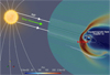 |
Fig. 1 Sketch of the magnetospheric interaction in the TRAPPIST-1–TRAPPIST-1e system. The stellar wind velocity and IMF streamlines are drawn in green and white, respectively. The M-dwarf star is shown as a yellow sphere, and the planet TRAPPIST-1e as a blue shaded circle. The planetary magnetic field lines (white) exhibit compression on the dayside and extension into a magnetotail. A bow shock structure forms upstream of the planet under a super-Alfvénic regime. The colour scale represents normalised plasma density. |
Input parameters used for the four simulated TRAPPIST-1e space weather scenarios.
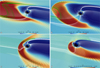 |
Fig. 2 Magnetospheric structures under four conditions: sub-Alfvénic (a), transition (b), super-Alfvénic (c), and CME conditions (d). The colour scale represents the density distribution of the solar wind. In the sub-Alfvénic regime (MA < 1), the stellar wind does not form a bow shock and the radio emission originates solely from magnetospheric reconnection. In the transition case, a weak and asymmetric shock begins to form. In the super-Alfvénic case (MA > 1), a clear bow shock develops, and the radio emission is strengthened by the shock and the reconnection region, the CME-like event, and a highly compressed and asymmetric magnetosphere. |
3.2 Habitability judgement: Magnetopause standoff distance
In this study we used the magnetopause standoff distance Rmsd as a diagnostic criterion to evaluate the magnetic shielding capability of TRAPPIST-1e. Specifically, we adopted a simplified threshold where Rmsd ≤ Re indicates insufficient protection of the planetary surface against the impinging stellar wind. This criterion has been employed in previous global MHD studies of magnetised exoplanets (Varela et al. 2022a,b; Peña-Moñino et al. 2024), where it serves as a practical proxy for assessing whether stellar wind particles can reach the surface and infer the habitability.
We note, however, that this approach neglects several important factors. The actual extent of a planet’s upper atmosphere can exceed Re depending on its composition, temperature profile, and extreme-ultraviolet environment, which can lead to atmospheric escape even if Rmsd > Re. Moreover, because the magnetopause surface is asymmetric, especially in tilted or compressed magnetospheres, the location where the IMF connects with planetary field lines varies with latitude. As a result, direct particle access to the upper atmosphere can occur in polar cusp regions even when the equatorial standoff distance is relatively large.
Despite these limitations, the Rmsd > Re criterion remains a widely used and computationally efficient first-order approximation for estimating whether magnetic shielding can prevent direct precipitation of stellar wind onto the surface. However, this picture may change when polar and cusp-related escape processes on magnetised planets are taken into account. Although an intrinsic magnetic field can shield the atmosphere from sputtering and ion pickup, it simultaneously opens up polar cap and cusp regions as escape channels, potentially enhancing the overall atmospheric loss rate. Increased stellar wind pressure and enhanced extreme-ultraviolet irradiation can lead to exosphere expansion, which further boosts escape rates (Lammer 2013). Notably, such expansion increases the rate of escape from both magnetised and un-magnetised planets, as the enlarged cusp area and higher ion production increase the flux along open field lines. Based on earlier models of exoplanetary escape, which considered only ion pickup and Jeans escape (Lammer et al. 2007), it was concluded that magnetisation is a prerequisite for habitability; however, when polar outflows and cusp escape are included, this conclusion may not hold (Gunell et al. 2018).
In most cases, the inner boundary is set at Rin = 2.0 Re. However, for simulations of extreme space weather – particularly CME-like scenarios, where the magnetosphere is significantly compressed and pressure gradients become steeper – we observe numerical instabilities when using this setting. To ensure stability, we adopted Rin = 1.5 Re specifically for the CME case. We considered TRAPPIST-1e unprotected if Rmsd ≤ 1.5 Re, as the magnetosphere fails to prevent direct stellar wind impact.
The value of Rmsd is determined from the simulation outputs by measuring the last closed magnetic field line in the substellar direction, as adopted in previous works (Varela et al. 2022b; Peña-Moñino et al. 2024), following the same methodology used in the analysis of Ganymede’s magnetosphere (Kivelson et al. 2004). This approach is simulation-based and does not rely on theoretical expressions. The theoretical standoff distance can be derived by equating the total pressure of the stellar wind with the pressure provided by the planetary magnetosphere. The stellar wind pressure includes the thermal pressure ![Mathematical equation: $\[P_{s w, t h}=m_{p} n_{s w} c_{s w}^{2} / \gamma\]$](/articles/aa/full_html/2025/09/aa55471-25/aa55471-25-eq22.png) , magnetic pressure
, magnetic pressure ![Mathematical equation: $\[P_{s w, m}=B_{s w}^{2} / 2 \mu_{0}\]$](/articles/aa/full_html/2025/09/aa55471-25/aa55471-25-eq23.png) , and dynamic pressure
, and dynamic pressure ![Mathematical equation: $\[P_{d}=m_{p} n_{s w} v_{s w}^{2} / 2\]$](/articles/aa/full_html/2025/09/aa55471-25/aa55471-25-eq24.png) . The planetary side includes its thermal pressure
. The planetary side includes its thermal pressure ![Mathematical equation: $\[P_{th,e}=m_{p} n_{e} v_{th,e}^{2} / 2\]$](/articles/aa/full_html/2025/09/aa55471-25/aa55471-25-eq25.png) , and magnetic pressure expressed as
, and magnetic pressure expressed as ![Mathematical equation: $\[P_{m, e}=\alpha \mu_{0} M_{p}^{2} / 8 \pi^{2} r^{6}\]$](/articles/aa/full_html/2025/09/aa55471-25/aa55471-25-eq26.png) . where Mp is the planetary magnetic moment, α is dipole compression coefficient (α ≈ 2; Gombosi 1994), and μ0 is the magnetic permeability.
. where Mp is the planetary magnetic moment, α is dipole compression coefficient (α ≈ 2; Gombosi 1994), and μ0 is the magnetic permeability.
Equating the total pressures, the theoretical expression for the normalised magnetopause standoff distance for TRAPPIST-1e (where Rp = Re) becomes
![Mathematical equation: $\[\frac{R_{\mathrm{msd}}}{R_p}=\left[\frac{\alpha M_p^2 / \pi}{m_p n_{\mathrm{sw}} v_{\mathrm{sw}}^2+\frac{B_{\mathrm{IMF}}^2}{4 \pi}+\frac{2 m_p n_{\mathrm{sw}} c_{\mathrm{sw}}^2}{\gamma}-m_p n_e v_{\mathrm{th}, \mathrm{e}}^2}\right]^{1 / 6}.\]$](/articles/aa/full_html/2025/09/aa55471-25/aa55471-25-eq27.png) (19)
(19)
It is important to emphasise that Eq. (19) provides only a rough theoretical estimate of the magnetopause distance (Rmsd) and may significantly deviate from the values obtained through global simulations or inferred from observations. Several key limitations must be considered when applying this expression. First, the derivation neglects the magnetic topology of the system. All terms in Eq. (19) are treated as scalar quantities, which oversimplifies the inherently vectorial and 3D nature of the stellar wind-magnetosphere interaction. In particular, the orientation of the IMF relative to the planetary dipole is not accounted for. As a result, the formula assumes a purely compressed dipole geometry, which does not represent realistic reconnection-driven magnetospheric configurations. Second, Eq. (19) does not include the effects of IMF–planetary field magnetic reconnection, which plays a critical role in controlling magnetospheric erosion and standoff distance. Third, while the theoretical expression yields a unique value for any given set of parameters nsw, vsw, BIMF, and Bp, our 3D MHD simulations reveal a range of magnetopause standoff distances depending on the tilt angle and the specific orientation of the IMF. This inherent variability reflects the complexity of magnetospheric dynamics and underlines the limitations of applying Eq. (19) as a general diagnostic. In extreme space weather cases or under strong reconnection conditions, the discrepancy between the theoretical and simulated values may be substantial. Therefore, while Eq. (19) can serve as an approximation, accurate determination of Rmsd requires 3D MHD modelling that includes both magnetic topology and reconnection, as presented in this work. In our simulations, magnetic reconnection arises from the intrinsic numerical diffusivity of the MHD solver. This approach has been shown to reproduce the essential large-scale features of magnetospheric erosion in previous studies (Varela et al. 2016c). However, it does not resolve kinetic-scale processes or localised current sheet dynamics and should be interpreted as a first-order approximation (Birn et al. 2001). Moreover, the model does not account for orbital motion, which could further influence the magnetospheric structure and reconnection dynamics, particularly for close-in exoplanets.
The procedure adopted to determine the magnetopause standoff distance Rmsd in this study is illustrated in Fig. 3. Although the simulation domain does not extend below Rin = 1.5 Re, the magnetopause standoff distance is defined as the distance from the planetary centre to the innermost closed magnetic field line projected onto the star–planet line (x-axis). The 3D location of this field line is extracted from the simulation output and geometrically projected in the original coordinate system. This approach yields an effective standoff distance that may fall below Rin, consistent with extreme magnetospheric compression. We emphasise that this value is geometric in nature and does not imply any numerical solution within the excluded inner domain.
The simulation and theoretical results for the magnetopause standoff distance (Rmsd) are illustrated in Fig. 4, which shows the outcomes under four different space weather scenarios, each evaluated with varying magnetic field strengths and tilt angles. For each condition, the simulations are organised to separately assess the effects of magnetic tilt and field strength on planetary habitability: first by fixing the planetary magnetic field and varying the tilt, and then by fixing the tilt and varying the magnetic field. These dual dependences are visualised in radar plots, where the two parameters can be interpreted simultaneously.
As seen in all four regimes, Rmsd decreases monotonically with increasing tilt angle and increases with stronger planetary magnetic fields. In favourable cases, the standoff distance can exceed 10 Re, which is sufficient to shield the planet from harmful stellar wind impacts, indicating a magnetospheric configuration supportive of habitability. The radial distance in each radar plot indicates the magnitude of Rmsd, and the three vertices correspond to three magnetic field strengths (0.32G, 0.64G, and 1.28 G) and three tilt angles (0°, 23.5°, and 45°).
In the Sub-Alfvénic case (top left), where the stellar magnetic pressure dominates (with B⋆ = 1200 G), the standoff distance reaches up to 9.7 Re, while under a weak field of 0.32 G and a tilt of 45°, it drops to 2.6 Re, approaching critical thresholds. This demonstrates that even in a magnetically dominated wind environment, weak planetary fields and large tilts can significantly compromise atmospheric protection.
In the transition regime (top right), where the stellar magnetic field is halved to 600 G, the magnetosphere exhibits the widest expansion among all cases. With a 1.28 G planetary field and zero tilt, Rmsd can reach 14.2 Re. However, increasing the tilt systematically reduces the standoff distance, reinforcing the trend that oblique fields weaken the planet’s magnetic shielding. Stronger magnetic fields, on the other hand, robustly enhance magnetospheric protection.
Under the super-Alfvénic condition (bottom left), where the stellar wind dynamic pressure exceeds the magnetic pressure, the magnetosphere becomes moderately compressed. The maximum Rmsd reaches 11.5 Re for a field strength of 1.28 G and 0° tilt. This emphasises the critical role of ram pressure in shaping the magnetospheric boundary.
The most extreme scenario (bottom right) corresponds to CME-like conditions, as outlined in Table 1, with greatly increased solar wind density, velocity, and IMF intensity. Here, the magnetosphere is severely compressed: the maximum Rmsd only reaches about 6 Re, and in the worst case (0.32 G, 45° tilt), it falls below the model’s inner boundary limit of 1.5 Re, reaching just 1.2 Re. This implies the planet would be directly exposed to the stellar wind, effectively losing magnetic protection even under moderate field strengths, particularly at high tilts.
We note that our simulation results, although broadly consistent with the theoretical trend of ![Mathematical equation: $\[R_{\mathrm{msd}} \propto B_p^{1 / 3}\]$](/articles/aa/full_html/2025/09/aa55471-25/aa55471-25-eq28.png) , deviate significantly in magnitude. While the standoff distance increases monotonically with field strength, the rate of increase does not strictly follow the one-third power law. This discrepancy arises from the assumptions embedded in the theoretical model, which idealises the magnetosphere as symmetric, static, and purely dipolar. It ignores key influences such as reconnection topology, magnetic field orientation, and 3D structure.
, deviate significantly in magnitude. While the standoff distance increases monotonically with field strength, the rate of increase does not strictly follow the one-third power law. This discrepancy arises from the assumptions embedded in the theoretical model, which idealises the magnetosphere as symmetric, static, and purely dipolar. It ignores key influences such as reconnection topology, magnetic field orientation, and 3D structure.
In our simulations, the planetary magnetic dipole is fixed in a planet-centred coordinate system, with the stellar wind flowing along the x-axis. To emulate the effect of magnetic obliquity, we varied the direction of the incoming IMF vector in the x − y plane. For instance, applying an IMF with both +x and +y components (i.e. pointing north-east in this frame) is geometrically equivalent to tilting the dipole clockwise in the x − y plane. This approach allows us to study effective magnetic obliquity without altering the internal magnetic field configuration. This affects both the reconnection efficiency and the global magnetospheric topology, leading to deviations from the static pressure balance. These effects are physically meaningful: the evolution of planetary magnetospheres is shaped by reconnection, magnetosheath dynamics, and boundary instabilities, all of which are naturally included in full 3D MHD models. Consequently, while the ![Mathematical equation: $\[B_p^{1 / 3}\]$](/articles/aa/full_html/2025/09/aa55471-25/aa55471-25-eq29.png) law provides a useful estimate, it has limitations in dynamically evolving or extreme space weather environments.
law provides a useful estimate, it has limitations in dynamically evolving or extreme space weather environments.
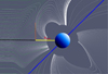 |
Fig. 3 Illustration of how the planetary magnetopause standoff distance (Rmsd) is measured in our simulations. The distance is defined as the last closed planetary magnetic field line along the star–planet line (here shown in yellow). The black and blue lines represent the radial direction and planetary magnetic axis, respectively. |
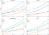 |
Fig. 4 Magnetopause standoff distance (Rmsd/Rp) of TRAPPIST-1e under four different stellar wind conditions: sub-Alfvénic (a), transition (b), super-Alfvénic (c), and CME-like (d). Each panel shows Rmsd as a function of planetary magnetic dipole strength (Bp = 0.32, 0.64, 1.28 G) for three magnetic axis tilt angles (0°, 23.5°, and 45°), with solid lines representing simulation results and dashed red lines indicating values predicted by the theoretical expression. In all scenarios, Rmsd increases with Bp and decreases with magnetic axis tilt. The transition case produces the largest magnetospheric extension, while the CME scenario exhibits the most severe compression, with Rmsd approaching ~1.5 Rp under the most unfavourable configurations, implying strong limitations on potential habitability. |
4 Radio emission from TRAPPIST-1e’s magnetosphere under various space weather conditions
The detection of radio emission generated by the magnetospheres of exoplanets remains one of the most promising observational methods for directly constraining their intrinsic magnetic fields, particularly in super-Alfvénic regimes where cyclotron maser emission can be efficiently excited. This has profound implications for understanding the internal structure and dynamics of exoplanets. Once the magnetic properties of an exoplanet are inferred, the space weather environment imposed by its host star along the planet’s orbit can be more thoroughly characterised. As a result, the strength of radio emission from the exoplanet’s magnetosphere is closely coupled with the ambient stellar wind conditions. Furthermore, numerical modelling of radio emission provides theoretical support for future observational campaigns targeting exoplanetary systems – particularly Earth-like planets or hot Jupiters – via radio interferometry, where magnetospheric SPIs may be detectable.
In this section we estimate the radio power emitted from the dayside magnetopause reconnection regions of TRAPPIST-1e under four different space weather conditions. The radio emission is computed based on our MHD simulations of the interaction between the stellar wind of the M dwarf TRAPPIST-1 and the planetary magnetic field of TRAPPIST-1e. This analysis represents one of the core goals of this study.
We adopted the radio-magnetic Bode’s law, in which the incident magnetised energy flux and the strength of the planetary magnetic obstacle determine the emitted radio power, expressed as P = βPB, where β is the empirical energy conversion efficiency, typically ranging from 2 to 10 × 10−3 (Zarka 2018). The dissipated power (PB) corresponds to the Poynting flux divergence in the dayside magnetosphere and is evaluated numerically by integrating over the volume between the bow shock nose and the magnetopause:
![Mathematical equation: $\[P=\beta P_B=\beta \int_V \nabla \cdot \frac{(V \times B) \times B}{4 \pi} \mathrm{~d} V.\]$](/articles/aa/full_html/2025/09/aa55471-25/aa55471-25-eq30.png) (20)
(20)
This integration method follows the approach described in Peña-Moñino et al. (2024), where PB is computed directly from the simulation outputs, and the only empirical assumption is the efficiency factor for converting dissipated power (β).
Electron cyclotron maser emission arises from energetic electrons accelerated along planetary magnetic field lines and may originate near the planet or propagate along Alfvén wings towards the star. The latter scenario typically occurs in sub-Alfvénic regimes, enabling SPI-induced emission. In contrast, planetary electron cyclotron maser emission can arise under both sub- and super-Alfvénic conditions.
In this study we focused on radio emission generated at the dayside, where the Poynting flux deposition is maximal. Previous numerical studies (Varela et al. 2016c, 2018) have shown that, under common stellar wind conditions, the radio power from the nightside (magnetotail) region is typically about an order of magnitude lower than that from the dayside. The contribution from auroral zones, however, remains uncertain in exoplanetary contexts due to the lack of direct observations and comprehensive modelling. We acknowledge that under certain conditions, auroral emissions could be significant, and future work is needed to evaluate their relative importance.
To avoid artificial artefacts near the numerical boundary, we defined the integration region with care, excluding volumes too close to the inner radial boundary. For simulations where a bow shock forms (i.e. super-Alfvénic and CME-like cases), the integration volume encompasses the entire dayside post-shock region, including the magnetosheath and magnetopause, where stellar wind kinetic energy is dissipated.
We computed the total dissipated magnetic power using Eq. (20) as a direct volume integral of the divergence of the Poynting flux, calculated from the MHD simulation output and evaluated in ParaView. The integration volume is constrained by three physical criteria: (1) the divergence of the Poynting flux is positive; (2) the plasma density exceeds the upstream stellar wind background value (n > nsw); and (3) the region lies immediately outside the inner boundary, where the dayside magnetopause typically forms. This approach ensures that the dominant energy dissipation regions are captured.
In Fig. 5 we illustrate the spatial distribution of magnetic energy dissipation, showing the separate volumetric contributions from the magnetopause (top) and the bow shock (bottom), in the regions identified by the applied density and energy flux thresholds. To distinguish regions of bow shock and magnetopause, we computed the density gradient along the x direction (∂n/∂x). A positive gradient indicates compression (e.g. near the bow shock), while a negative gradient is associated with plasma rarefaction (e.g. behind the magnetopause).
Figure 6 presents the simulated radio power (P) of TRAPPIST-1e under four different space weather regimes. In the sub-Alfvénic and transition regimes, no bow shock forms. Radio emission therefore arises solely from reconnection at the planetary magnetopause. In the super-Alfvénic regime, both a magnetopause and bow shock exist, and energetic electrons are generated in both regions. This results in combined radio contributions linked to IMF pileup and bending. For simplicity, we report only the total emission (magnetopause plus bow shock) in all panels of Fig. 6.
In the sub-Alfvénic case (Fig. 6a), the maximum radio power reaches 1.25 × 10¹⁹ erg s−1 for Bp = 1.28 G and a tilt angle of 45°. The emission decreases with lower Bp and smaller tilt angles, indicating the crucial role of magnetic configuration in determining emission efficiency. In the transition case (MA ~ 1; Fig. 6b), the maximum radio output is the lowest among the calm space weather cases, reaching only 8.9 × 10¹⁸ erg s−1 under strong field and large tilt. This reduction can be attributed to weaker stellar wind forcing and topological distortion near the magnetopause, reducing reconnection efficiency.
In the super-Alfvénic regime (Fig. 6c, enhanced dynamic pressure produces a more compact and active magnetosphere. The maximum emission reaches 4.5 × 10¹⁹ erg s−1 for Bp = 1.28 G, while for weaker fields, the emission drops below 1.0 × 10¹⁹ erg s−1. The emission increases with tilt, implying stronger reconnection along displaced magnetic shear regions.
In the CME-like regime (Fig. 6d), the stellar wind exhibits significantly higher speed, density, and IMF strength. The radio emission peaks at 9 × 10²⁰ erg s−1 – the strongest among all scenarios – reflecting extreme compression and reconnection enhancement driven by CME conditions.
In summary, our simulations demonstrate that TRAPPIST-1e’s radio emission is highly sensitive to both internal planetary parameters (magnetic field strength and tilt) and external space weather drivers. The CME-like scenario in particular stands out as a potential high-emission target for exoplanetary radio detection.
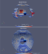 |
Fig. 5 Contribution to the radio emission from the magnetopause (upper) and bow shock (bottom) regions of TRAPPIST-1e derived from our simulation. The volumetric distributions represent the dissipated magnetic energy flux (Poynting flux, Pw), highlighting the intensity and spatial structure of energy dissipation responsible for planetary radio emission under stellar wind interaction conditions. |
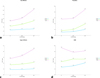 |
Fig. 6 Radio emission plots of TRAPPIST-1e under four different space weather conditions: sub-Alfvénic (a), transition (b), super-Alfvénic (c), and CME-like (d). The horizontal axis shows the inclination of the magnetic axis, the different colours represent different magnetic field strengths, and the vertical axis indicates the radiated power (in erg s−1). The results were obtained using the empirical factor β. |
5 Conclusions
In this study we conducted a comprehensive investigation of the magnetospheric response and radio emission properties of the Earth-sized exoplanet TRAPPIST-1e under a range of stellar wind conditions, using 3D MHD simulations implemented with the PLUTO 4.4 code. Our simulation framework captures both the magnetic and fluid dynamics of the planetary magnetosphere in interaction with the IMF, providing insights into the standoff distance of the magnetopause and the associated Poynting flux that drives radio emission.
We evaluated four representative space weather scenarios: the sub-Alfvénic regime, a transitional regime near the Alfvén surface, a super-Alfvénic regime, and an extreme CME-like event. In each case, we varied planetary magnetic field strengths and magnetic axis tilt angles to explore how the internal planetary configuration modulates the resulting magnetospheric structure and energy dissipation.
Our simulations reveal that the magnetopause standoff distance (Rmsd) grows monotonically with increasing planetary magnetic field strength, though the rate of this growth does not strictly follow the canonical law predicted by idealised pressure balance models, ![Mathematical equation: $\[R_{\mathrm{msd}} \propto B_p^{1 / 3}\]$](/articles/aa/full_html/2025/09/aa55471-25/aa55471-25-eq31.png) . This deviation arises due to complex 3D magnetospheric topology, asymmetric reconnection, and the presence of boundary instabilities. These effects indicate that realistic modelling of exoplanetary space environments must go beyond static pressure balance to include topological and dynamic phenomena.
. This deviation arises due to complex 3D magnetospheric topology, asymmetric reconnection, and the presence of boundary instabilities. These effects indicate that realistic modelling of exoplanetary space environments must go beyond static pressure balance to include topological and dynamic phenomena.
A key component of this work is the estimation of radio emission arising from dayside magnetospheric reconnection, using the radiomagnetic Bode law, P = βPB, with β = 2 × 10⁻³, as the adopted efficiency. We integrated the divergence of the Poynting vector within the region bounded by the bow shock and magnetopause to determine the dissipated magnetic energy available for particle acceleration. These estimates reveal that TRAPPIST-1e could generate high levels of coherent radio emission under suitable stellar wind conditions. For example, under extreme CME-like conditions, the total radio power reaches as high as 9 × 10²⁰ erg/s, while in the more moderate sub-Alfvénic case, peak emission is around 1.2 × 10¹⁹ erg/s for favourable planetary parameters and can reach 4.5 × 10¹⁹ erg/s for super-Alfvénic.
We find that the planetary magnetic field strength primarily determines radio power output but that the tilt angle also plays a significant modulating role, especially in sub- and super-Alfvénic regimes. Despite the promising levels of radio emission predicted by our models, the majority of these signals are expected to fall below the ionospheric cutoff frequency of Earth (typically around 10 MHz) since the emission frequency is determined by the local electron cyclotron frequency, fce = 2.8 B [G] MHz, which depends on the planetary magnetic field strength. For Earth-like planets such as TRAPPIST-1e, the maximum field strength considered here (Bp = 1.28 G) typically results in a maximum electron cyclotron frequency of fce < 10 MHz, making ground-based detection challenging due to the Earth’s ionospheric cutoff. In contrast, hot Jupiters with magnetic fields of several tens of gauss can emit above this threshold and thus remain viable candidates for radio detection. This implies that such emissions would not be detectable by groundbased radio telescopes if TRAPPIST-1e possesses a magnetic field strength similar to Earth’s (~0.3 G). However, space-based or lunar-surface radio arrays operating at low frequencies could overcome this limitation and represent a compelling avenue for future detection efforts. Our results also underscore the potential detectability of more magnetically active exoplanets, such as hot Jupiters, which may produce emission above the ionospheric cutoff.
Looking forward, space missions such as China’s proposed Discovering the Sky at the Longest Wavelength (DSL) array (also known as the Hongmeng Project) on the lunar far side provide promising platforms for such low-frequency exoplanetary radio studies (Chen et al. 2023). In parallel, new advances in domestic instrumentation such as the FAST Core Array project (Jiang et al. 2024) could enhance detection capability in higher-frequency regimes, aiding the search for bursty or harmonically up-shifted exoplanetary emissions. In summary, our study demonstrates that the interaction between TRAPPIST-1e and the stellar wind environment of TRAPPIST-1 has the potential to generate significant magnetospheric radio signals, depending on planetary magnetic parameters and external space weather forcing. These signals, though likely inaccessible to ground-based observatories, offer exciting prospects for future space-based detection and contribute to our broader understanding of planetary magnetism, habitability, and SPIs.
Acknowledgements
This work is supported by National Natural Science Foundation of China (Grant No. 42274221), The Leading Talents of Guangdong Province Program (Grant No. 2021CX02Z468), National Key R&D Program of China (No. 2022YFF0503800), and Center for Computational Science and Engineering at Southern University of Science and Technology.
References
- Airapetian, V. S., Barnes, R., Cohen, O., et al. 2020, Int. J. Astrobiol., 19, 136 [NASA ADS] [CrossRef] [Google Scholar]
- Birn, J., Drake, J. F., Shay, M. A., et al. 2001, J. Geophys. Res., 106, 3715 [Google Scholar]
- Bourrier, V., de Wit, J., Bolmont, E., et al. 2017, AJ, 154, 121 [NASA ADS] [CrossRef] [Google Scholar]
- Büchner, J., & Zelenyi, L. M. 1987, J. Geophys. Res., 92, 2565 [Google Scholar]
- Büchner, J., Dum, C. T., & Scholer, M. 2003, in Space Plasma Simulation, eds. J. Büchner, C. T. Dum, & M. Scholer (Berlin Heidelberg: Springer Verlag) [Google Scholar]
- Bunescu, C., Vogt, J., Marghitu, O., et al. 2019, Ann. Geophys., 37, 347 [NASA ADS] [CrossRef] [Google Scholar]
- Chen, X., Yan, J., Xu, Y., et al. 2023, Chinese J. Space Sci., 43, 43 [Google Scholar]
- Dedner, A., Kemm, F., Kröner, D., et al. 2002, J. Comput. Phys., 175, 645 [Google Scholar]
- de Keyser, J., Dunlop, M. W., Owen, C. J., et al. 2005, Space Sci. Rev., 118, 231 [NASA ADS] [CrossRef] [Google Scholar]
- Dong, C., Jin, M., Lingam, M., et al. 2018, Proc. Natl. Acad. Sci., 115, 260 [NASA ADS] [CrossRef] [Google Scholar]
- Garraffo, C., Drake, J. J., Cohen, O., et al. 2017, ApJ, 843, L33 [Google Scholar]
- Gillon, M., Jehin, E., Lederer, S. M., et al. 2016, Nature, 533, 221 [Google Scholar]
- Gillon, M., Triaud, A. H. M. J., Demory, B.-O., et al. 2017, Nature, 542, 456 [NASA ADS] [CrossRef] [Google Scholar]
- Goertz, C. K. 1980, J. Geophys. Res., 85, 2949 [NASA ADS] [CrossRef] [Google Scholar]
- Goldreich, P., & Lynden-Bell, D. 1969, ApJ, 156, 59 [Google Scholar]
- Gombosi, T. I. 1994, Gaskinetic Theory, Cambridge Atmospheric and Space Science Series (Cambridge: Cambridge University Press), 9 [Google Scholar]
- Gunell, H., Liu, K., Karlsson, T., et al. 2018, A&A, 615, A141 [NASA ADS] [CrossRef] [EDP Sciences] [Google Scholar]
- Hess, S. L. G., & Zarka, P. 2011, A&A, 531, A29 [NASA ADS] [CrossRef] [EDP Sciences] [Google Scholar]
- Jakosky, B. M., Grebowsky, J. M., Luhmann, J. G., et al. 2015, Geophys. Res. Lett., 42, 8791 [NASA ADS] [CrossRef] [Google Scholar]
- Jiang, P., Chen, R. R., Gan, H. Q., et al. 2024, Astron. Tech. Instrum., 1, 84 [CrossRef] [Google Scholar]
- Kivelson, M. G., Bagenal, F., Kurth, W. S., et al. 2004, Jupiter. The Planet, Satellites and Magnetosphere (Cambridge: Cambridge University Press), 513 [Google Scholar]
- Lammer, H., Lichtenegger, H. I. M., Kulikov, Y. N., et al. 2007, Astrobiology, 7, 185 [NASA ADS] [CrossRef] [Google Scholar]
- Lammer, H. 2013, Origin and Evolution of Planetary Atmospheres: Implications for Habitability (Berlin Heidelberg: Springer-Verlag) [Google Scholar]
- Mignone, A., Bodo, G., Massaglia, S., et al. 2007, ApJS, 170, 228 [Google Scholar]
- Neubauer, F. M. 1980, J. Geophys. Res., 85, 1171 [Google Scholar]
- Peña-Moñino, L., Pérez-Torres, M., Varela, J., et al. 2024, A&A, 688, A138 [NASA ADS] [CrossRef] [EDP Sciences] [Google Scholar]
- Pérez-Torres, M., Gómez, J. F., Ortiz, J. L., et al. 2021, A&A, 645, A77 [NASA ADS] [CrossRef] [EDP Sciences] [Google Scholar]
- Pineda, J. S., & Villadsen, J. 2023, Nat. Astron., 7, 569 [NASA ADS] [CrossRef] [Google Scholar]
- Réville, V., Jasinski, J. M., Velli, M., et al. 2024, ApJ, 976, 65 [CrossRef] [Google Scholar]
- Ridley, A. J., De Zeeuw, D. L., Manchester, W. B., et al. 2006, Adv. Space Res., 38, 263 [NASA ADS] [CrossRef] [Google Scholar]
- Ritter, P., Lühr, H., & Rauberg, J. 2013, Earth Planets Space, 65, 1285 [NASA ADS] [CrossRef] [Google Scholar]
- Samsonov, A. A., Gordeev, E., Tsyganenko, N. A., et al. 2016, J. Geophys. Res. Space Phys., 121, 6493 [Google Scholar]
- Trigilio, C., Biswas, A., Leto, P., et al. 2023, arXiv e-prints [arXiv:2305.00809] [Google Scholar]
- Turner, J. D., Zarka, P., Grießmeier, J.-M., et al. 2021, A&A, 645, A59 [NASA ADS] [CrossRef] [EDP Sciences] [Google Scholar]
- Varela, J., Pantellini, F., & Moncuquet, M. 2015, Planet. Space Sci., 119, 264 [NASA ADS] [CrossRef] [Google Scholar]
- Varela, J., Pantellini, F., & Moncuquet, M. 2016a, Planet. Space Sci., 122, 46 [NASA ADS] [CrossRef] [Google Scholar]
- Varela, J., Pantellini, F., & Moncuquet, M. 2016b, Planet. Space Sci., 120, 78 [NASA ADS] [CrossRef] [Google Scholar]
- Varela, J., Araneda, J. A., & Zimbardo, G. 2016c, A&A, 595, A108 [NASA ADS] [CrossRef] [EDP Sciences] [Google Scholar]
- Varela, J., Réville, V., Brun, A. S., et al. 2018, A&A, 616, A182 [NASA ADS] [CrossRef] [EDP Sciences] [Google Scholar]
- Varela, J., Brun, A. S., Strugarek, A., et al. 2022a, A&A, 659, A10 [NASA ADS] [CrossRef] [EDP Sciences] [Google Scholar]
- Varela, J., Brun, A. S., Zarka, P., et al. 2022b, Space Weather, 20, e2022SW003164 [NASA ADS] [CrossRef] [Google Scholar]
- Wheatley, P. J., Louden, T., Bourrier, V., et al. 2017, MNRAS, 465, L74 [NASA ADS] [CrossRef] [Google Scholar]
- Waters, C. L., Anderson, B. J., & Liou, K. 2001, Geophys. Res. Lett., 28, 2165 [NASA ADS] [CrossRef] [Google Scholar]
- Weimer, D. R. 2001, J. Geophys. Res., 106, 12889 [Google Scholar]
- Zarka, P. 2018, Handbook of Exoplanets (Berlin: Springer), 22 [Google Scholar]
- Zhang, Q.-H., Zhang, Y.-L., Wang, C., et al. 2020, Proc. Natl. Acad. Sci., 117, 16193 [Google Scholar]
All Tables
Input parameters used for the four simulated TRAPPIST-1e space weather scenarios.
All Figures
|
Fig. 1 Sketch of the magnetospheric interaction in the TRAPPIST-1–TRAPPIST-1e system. The stellar wind velocity and IMF streamlines are drawn in green and white, respectively. The M-dwarf star is shown as a yellow sphere, and the planet TRAPPIST-1e as a blue shaded circle. The planetary magnetic field lines (white) exhibit compression on the dayside and extension into a magnetotail. A bow shock structure forms upstream of the planet under a super-Alfvénic regime. The colour scale represents normalised plasma density. |
| In the text | |
|
Fig. 2 Magnetospheric structures under four conditions: sub-Alfvénic (a), transition (b), super-Alfvénic (c), and CME conditions (d). The colour scale represents the density distribution of the solar wind. In the sub-Alfvénic regime (MA < 1), the stellar wind does not form a bow shock and the radio emission originates solely from magnetospheric reconnection. In the transition case, a weak and asymmetric shock begins to form. In the super-Alfvénic case (MA > 1), a clear bow shock develops, and the radio emission is strengthened by the shock and the reconnection region, the CME-like event, and a highly compressed and asymmetric magnetosphere. |
| In the text | |
|
Fig. 3 Illustration of how the planetary magnetopause standoff distance (Rmsd) is measured in our simulations. The distance is defined as the last closed planetary magnetic field line along the star–planet line (here shown in yellow). The black and blue lines represent the radial direction and planetary magnetic axis, respectively. |
| In the text | |
|
Fig. 4 Magnetopause standoff distance (Rmsd/Rp) of TRAPPIST-1e under four different stellar wind conditions: sub-Alfvénic (a), transition (b), super-Alfvénic (c), and CME-like (d). Each panel shows Rmsd as a function of planetary magnetic dipole strength (Bp = 0.32, 0.64, 1.28 G) for three magnetic axis tilt angles (0°, 23.5°, and 45°), with solid lines representing simulation results and dashed red lines indicating values predicted by the theoretical expression. In all scenarios, Rmsd increases with Bp and decreases with magnetic axis tilt. The transition case produces the largest magnetospheric extension, while the CME scenario exhibits the most severe compression, with Rmsd approaching ~1.5 Rp under the most unfavourable configurations, implying strong limitations on potential habitability. |
| In the text | |
|
Fig. 5 Contribution to the radio emission from the magnetopause (upper) and bow shock (bottom) regions of TRAPPIST-1e derived from our simulation. The volumetric distributions represent the dissipated magnetic energy flux (Poynting flux, Pw), highlighting the intensity and spatial structure of energy dissipation responsible for planetary radio emission under stellar wind interaction conditions. |
| In the text | |
|
Fig. 6 Radio emission plots of TRAPPIST-1e under four different space weather conditions: sub-Alfvénic (a), transition (b), super-Alfvénic (c), and CME-like (d). The horizontal axis shows the inclination of the magnetic axis, the different colours represent different magnetic field strengths, and the vertical axis indicates the radiated power (in erg s−1). The results were obtained using the empirical factor β. |
| In the text | |
Current usage metrics show cumulative count of Article Views (full-text article views including HTML views, PDF and ePub downloads, according to the available data) and Abstracts Views on Vision4Press platform.
Data correspond to usage on the plateform after 2015. The current usage metrics is available 48-96 hours after online publication and is updated daily on week days.
Initial download of the metrics may take a while.