| Issue |
A&A
Volume 701, September 2025
|
|
|---|---|---|
| Article Number | A53 | |
| Number of page(s) | 14 | |
| Section | The Sun and the Heliosphere | |
| DOI | https://doi.org/10.1051/0004-6361/202555534 | |
| Published online | 02 September 2025 | |
Modelling gyrosynchrotron emission from coronal energetic electrons in a CME flux rope
1
Centre for mathematical Plasma Astrophysics, Department of Mathematics, KU Leuven, Celestijnenlaan 200B, 3001 Leuven, Belgium
2
Department of Physics and Astronomy, University of Turku, 20014 Turku, Finland
3
The Johns Hopkins University Applied Physics Laboratory, 11001 Johns Hopkins Rd, 20723 Laurel, USA
4
Institute of Physics, University of Maria Curie-Skłodowska, Pl. Marii Curie-Skłodowskiej 1, 20-031 Lublin, Poland
⋆ Corresponding author: This email address is being protected from spambots. You need JavaScript enabled to view it.
Received:
16
May
2025
Accepted:
21
July
2025
Abstract
Context. Solar flares and coronal mass ejections (CMEs) can accelerate electrons, causing bursts such as type IV emissions in the solar radio continuum. Although radio spectroscopy is a powerful diagnostic tool for the corona, the origin and mechanisms of type IV bursts remain uncertain. In situ measurements can occasionally shed some light on these mechanisms, but they are limited in space and time. Sophisticated numerical modelling offers the best approach to improve our understanding of the physical processes underlying particle dynamics and radio emission.
Aims. This research examines type IV radio bursts, exploring the effects of various electron distribution properties and CMEs on their generation and characteristics. To transcend idealised assumptions, we employed realistic anisotropic electron distributions – obtained from particle transport simulations within complex magnetohydrodynamic (MHD) environments – as input for radio emission models.
Methods. We used the three-dimensional coronal MHD model COCONUT to generate coronal background configurations, including a CME modelled as an unstable modified Titov–Démoulin magnetic flux rope (MFR). These MHD simulations were used by the PARADISE particle transport code, which injects energetic electrons into the MFR and tracks their evolution. Finally, we fed the electron distributions and solar wind parameters into the Ultimate Fast Gyrosynchrotron Codes to compute radio emission along lines of sight.
Results. Electrons injected close to the flux rope’s central axis remained largely confined, producing a gyrosynchrotron emission spectrum resembling observed type IV characteristics. Varying observer positions, CME properties, and spectral indices of the electron energy distributions modified the intensities and durations of the observed bursts. The strongest gyrosynchrotron emission was observed as originating from the CME flanks.
Conclusions. Our results indicate that gyrosynchrotron emission is the major component in type IV spectra, although additional contributors cannot be ruled out.
Key words: Sun: corona / Sun: coronal mass ejections (CMEs) / Sun: particle emission / Sun: radio radiation
© The Authors 2025
 Open Access article, published by EDP Sciences, under the terms of the Creative Commons Attribution License (https://creativecommons.org/licenses/by/4.0), which permits unrestricted use, distribution, and reproduction in any medium, provided the original work is properly cited.
This article is published in open access under the Subscribe to Open model. This email address is being protected from spambots. You need JavaScript enabled to view it. to support open access publication.
1. Introduction
The solar corona is a highly dynamic environment, characterised by spatio-temporal variations that manifest across its broadband electromagnetic spectrum, extending from radio wavelengths to gamma rays. Fundamental plasma processes in the corona give rise to diverse radiative phenomena and are broadly categorised by how individual electrons contribute to the observed radiation (Kundu 1965). A common classification distinguishes between coherent and incoherent emissions (Kaplan & Tsytovich 1969). In coherent emission, many thermal or nonthermal electrons act collectively, producing phase-correlated waves. This collective behaviour can lead to highly amplified and organised bursts of radiation (Zheleznyakov 1970; Melrose 1980, 2017). In contrast, incoherent emission occurs when electrons radiate independently with random phases, resulting in more gradual and less intense radiation (Schwinger 1949; Born & Wolf 1959; Ginzburg & Syrovatskii 1964). These classifications relate to the underlying emission mechanisms. Spontaneous emission, for instance, occurs when electrons radiate independently, typically resulting in incoherent radiation. Induced (or stimulated) emission, on the other hand, happens when incident radiation triggers electrons to emit additional phase-aligned radiation, often leading to coherent bursts (Galeev et al. 1965; Litvak & Trakhtengerts 1971; Papadopoulos & Freund 1979).
Under typical coronal conditions, and more broadly in space plasmas, characteristic plasma frequencies, such as the electron plasma frequency and the electron gyrofrequency, fall within the radio regime, making radio observations a powerful diagnostic tool (Nindos 2020). Spontaneous, incoherent processes generally dominate in thermal plasmas. In contrast, spontaneous and induced processes may occur in nonthermal environments, such as during solar flares, giving rise to a rich variety of radio emission features (Pick & Vilmer 2008). This diversity of solar radio emission is categorised into four primary types, formally labelled as types I – IV. During extreme releases of the Sun’s magnetic energy, whether through solar flares or coronal mass ejections (CMEs), all types of radio emissions may be observed, providing a unique window into high-energy physics that remains inaccessible at other wavelengths (Knock & Cairns 2005; Jebaraj et al. 2021, 2023, 2024; Alissandrakis et al. 2021; Klein et al. 2022; Wilson et al. 2025). This makes radio emission a valuable probe of the acceleration, release, and transport of solar energetic particles (SEPs). However, only energetic electrons directly produce radio emissions that are detectable from the solar atmosphere (Kouloumvakos et al. 2015).
Solar radio emissions have been studied extensively (e.g. Melrose 1980; Gary & Keller 2004), but several fundamental questions remain. An enduring conundrum involves the origin of type IV bursts which are associated with energetic eruptions. The name type IV refers to both a broadband continuum and the bursty emission that may occur within it. It is important to distinguish the two because their emission mechanisms are believed to be fundamentally different and to occur under distinct conditions. Figure 1 shows a dynamic radio spectrum of a type IV burst recorded by the Sagamore Hill Radio Observatory on 24 September 2011 (Kumari 2022). The spectrum displays several features commonly observed in type IV bursts, including a gradual drift of the peak intensity toward lower frequencies over time (above 125 MHz), stationary (in frequency) structures (between 25 and 50 MHz), and a bursty, high-intensity core surrounded by regions of weaker emission. While the depicted type IV burst lasted around 5 hours, typical durations of type IVs range from minutes to about an hour (Robinson 1978; Gergely 1986).
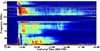 |
Fig. 1. Dynamic radio spectrum of a type IV radio burst detected by the Sagamore Hill Solar Radio Observatory on 24 September 2011. Adapted from Kumari (2022). |
Type IV emissions are subdivided into moving and stationary spectral types, referred to as type IVm and type IVs, respectively (e.g. Vourlidas 2004, and references therein). Type IVm can be synchrotron, gyrosynchrotron (GS), or plasma emission of electrons entrained within CMEs (e.g. Dulk 1973). Type IVs radio bursts are usually attributed to plasma emission (Melrose 1980). Historically, spectral drift has often been interpreted as a proxy for radio source motion, with spectral drift implying spatial motion of the emission region (Weiss 1963; Robinson 1978; Zlotnik et al. 2003; Chernov 2006; Nishimura et al. 2013; Bain et al. 2014; Kumari et al. 2021) and the absence of spectral drift suggesting a stationary source (Weiss 1963; Robinson & Smerd 1975; Dulk 1985; Lv et al. 2021). However, it should be noted that imaging observations have suggested that both (spectrally defined) IVm and IVs continua can exhibit spatial drift (Koval et al. 2016; Salas-Matamoros & Klein 2020; Morosan et al. 2021). In addition, Lv et al. (2021) have reported frequency-dependent spatial structuring for IVs events, possibly reflecting embedded CMEs. Furthermore, Kumari et al. (2021) found in their study that while most CMEs were accompanied by type IV bursts, only a minority of these were actually of the moving type. If such a spectral and spatial decorrelation exists in type IV behaviour, it must be an intrinsic property of the source itself.
Nonthermal electrons accelerated during CME eruptions can emit GS radiation if they remain trapped within an erupting flux rope or plasmoid. This type of emission, sometimes referred to as a ’radio CME’, differs from the radiation originating at shock fronts or from remote flare loops. Relativistic electrons (with Lorentz factors  , where γ = (1 − v2/c2)−1/2) spiralling along solar magnetic field lines produce GS radiation, whereas ultra-relativistic electrons (
 ) generate synchrotron emission. According to standard theory, GS emission occurs in magnetoactive plasma environments where dispersive effects significantly modify the radiation and must be considered (Melrose 1968; Zheleznyakov 1969). In contrast, pure synchrotron emission is typically treated as a vacuum process, and it is appropriate when plasma densities are low or emission frequencies are high enough to minimise medium-related effects (Schwinger 1949; Ginzburg 1979).
For these reasons, type IVm bursts have an important space weather aspect, as they carry information of the magnetic content of the CME (Vourlidas et al. 2020). However, they have been difficult to detect and study. Coherent emissions tend to dominate the radio spectra during eruptions, hindering the detection of faint emission from the CME interior. Joint white-light and radio observations of transients were rare until the launch of the Solar and Heliospheric Observatory (SOHO) in the mid-1990s. Soon after, Bastian et al. (2001) reported the first direct radio imaging of a white-light CME, revealing a moving radio source within the CME with a spectrum consistent with GS emission. The study obtained the spatial distribution of energetic electrons within the CME and an estimate of the CME’s internal magnetic field strength and electron population. Since then, several additional events have been detected (Maia et al. 2007; Tun & Vourlidas 2013; Mondal et al. 2020; Kansabanik et al. 2024).
A key research focus in type IV bursts is using their emission to estimate CME magnetic fields, which are nearly impossible to assess by other means (Morosan et al. 2019; Kumari et al. 2021). Various studies have interpreted GS emission as the primary mechanism in type IV radio bursts to infer magnetic field strengths within CMEs at specific solar radial distances (Gopalswamy & Kundu 1987; Bastian et al. 2001; Maia et al. 2007; Tun & Vourlidas 2013; Bain et al. 2014; Hariharan et al. 2016; Carley et al. 2017). However, significant uncertainties remain regarding the inferred magnetic field strengths and the detailed relationship between CMEs and type IV radio bursts, particularly when relying solely on remote observational methods (Morosan et al. 2019; Kumari et al. 2021).
Numerical models capable of realistically reproducing complex solar wind structures and simulating the acceleration and transport of energetic particles, combined with radio emission models, can help address open questions regarding the mechanisms underlying particle acceleration and radio emission. We demonstrate this approach in this work by coupling three numerical models to simulate GS emission from energetic electrons, including mildly relativistic and ultra-relativistic populations trapped within an erupting flux rope. We deployed the first-principles magnetohydrodynamical (MHD) coronal model COolfluid COroNal UnsTructured (COCONUT; Perri et al. 2022) constrained by observational magnetogram data at the inner boundary to generate realistic coronal conditions. This model represents the CME as an unstable Titov–Démoulin magnetic flux rope (MFR; Titov & Démoulin 1999; Titov et al. 2014). The transport of energetic electrons was modelled via the physics based PArticle Radiation Asset Directed at Interplanetary Space Exploration (PARADISE) model (Wijsen et al. 2019; Wijsen 2020), which has been coupled to COCONUT previously (Husidic et al. 2024). The MHD parameters derived from COCONUT and electron distributions obtained from PARADISE were then passed into the Ultimate Fast Gyrosynchrotron Codes (UFGSCs; Fleishman & Kuznetsov 2010; Kuznetsov & Fleishman 2021) to derive synthetic type IV radio spectra by computing the full GS emission and absorption coefficients using fast and accurate numerical approximations. By varying electron injection spectra and MFR configurations, and observing the evolving CME from different vantage points in the solar corona, we investigate how electron and CME properties influence the characteristics of radio spectra, including intensity, spectral shape, duration, and frequency range.
The remainder of the paper is structured as follows. In Sect. 2, we describe the coupled numerical models used to generate synthetic radio spectra. Simulation results are presented and discussed in Sect. 3, and we conclude with a summary and outlook in Sect. 4. Additional technical details of the numerical models are provided in the Appendix A.
2. Coupled numerical models and setup
Figure 2 illustrates the modelling chain to generate synthetic radio spectra, represented as a flowchart and described in the following subsections. The process began by computing a relaxed corona using the MHD model COCONUT and an HMI magnetogram. The simulation was then restarted with a superimposed unstable MFR to represent the CME1. Next, the particle transport code PARADISE was used to evolve energetic electron distributions within the MHD environment. Finally, the synthetic GS emission was computed by combining the electron distributions from PARADISE and plasma parameters from COCONUT as input to the GS radiation code.
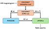 |
Fig. 2. Illustration of the modelling chain for the generation of synthetic radio spectra. |
2.1. The COCONUT model
COCONUT is a 3D MHD model that solves the ideal MHD equations in a time-implicit manner, producing realistic coronal configurations. In this work, we used the recently updated version of COCONUT, which incorporates additional source terms for coronal heating, radiation losses, and thermal conduction into the energy conservation equation (Baratashvili et al. 2024). The generation of the coronal background proceeded in two stages. First, we computed the relaxed background solar wind using a magnetogram obtained from the Helioseismic and Magnetic Imager (HMI) on board the Solar Dynamics Observatory, dated July 2, 2019. We then restarted the COCONUT simulation, modifying only the magnetic field by superimposing an MFR at the solar surface. The magnetogram was taken from a period of solar minimum, providing a less complex coronal environment that minimised additional influences on the evolution of the CME and the energetic particle distribution.
The CME can be characterised by a dimensionless parameter ζ. Generally, larger values of ζ correspond to more free magnetic energy, leading to more violent CMEs with higher injection speeds and stronger magnetic fields (see Appendix A.1 for details). In this work, we used two setups: one with ζ = 30 and one with ζ = 70. The case ζ = 30 produced a CME with an initial magnetic field strength of about 5.8 G and an initial speed of about 9.4 × 107 cm/s, whereas the case ζ = 70 resulted in a CME with a stronger field of about 10.6 G and a faster speed of roughly 1.3 × 108 cm/s. The remaining parameters for the two CMEs used in the Titov–Démoulin model were identical (see Appendix A.1).
2.2. The PARADISE code
Next, the particle transport code PARADISE was employed to inject and propagate energetic electron distributions within the erupting MFR. The electron distributions evolved according to the focused transport equation (FTE; e.g. van den Berg et al. 2020), which governs their anisotropic evolution by accounting for particle scattering, focusing, mirroring, and adiabatic deceleration, among other effects. Hence, PARADISE enabled us to track the development of electron distributions in both pitch-angle and energy space along the evolving MFR, capturing the interplay between magnetic field variations and particle transport.
We selected two different spectral indices for the electron injection spectra. Assuming a power-law energy distribution dN/dE ∝ E−δ, we chose δ = 2 and δ = 3 with an initial energy range from 10 keV to 10 MeV and isotropic pitch-angle distribution. The electrons were injected as a delta function in time, approximately 30 minutes after the CME’s eruption, within one of the CME flanks (i.e. the side regions of the MFR, curving downward from the apex) near its central axis and about 0.5 R⊙ above the solar surface. We adopted an injection method similar to that used by Husidic et al. (2024), in which a specified high magnetic field value is used to identify the injection site. This approach has previously proven effective to ensure particle confinement within the CME. The selected energy range is motivated by previous studies identifying 10 keV to 10 MeV as relevant for GS emission (Dulk & Marsh 1982; Fleishman & Kuznetsov 2010; Kuznetsov & Fleishman 2021), while spectral indices δ ≥ 2 are commonly observed (e.g. Maksimovic et al. 1997) and frequently adopted in GS calculations and modelling (e.g. Dulk 1973; Dulk & Marsh 1982; Kuznetsov & Fleishman 2021). At injection time, the CME reached a height of about 2.7 R⊙ for ζ = 30, and for ζ = 70, approximately 3.9 R⊙. By the end of the simulation, the corresponding CME heights were about 8.1 R⊙ and 13.1 R⊙, respectively.
The simulation results from PARADISE are expressed as differential intensities, j, from which the particle distribution function f can be derived according to
 (1)
(1)
with spatial vector x, momentum magnitude p, pitch-angle cosine μ = cos α and pitch-angle α, and time t. Because the FTE is linear, its solutions can be scaled by an arbitrary constant. In Appendix A.2 we describe the required units for the GS code and how they are obtained.
2.3. The Ultimate Fast GS Codes
The UFGSCs contain a set of numerical schemes for calculating GS emission in the non-quantum regime, covering non-relativistic (γ ≈ 1), mildly relativistic (γ ≳ 1), and ultra-relativistic (γ ≫ 1) energy ranges (Kuznetsov & Fleishman 2021). While an earlier version of these GS codes was limited to using idealised (i.e. analytically defined) distribution functions in energy and pitch-angle cosine (Fleishman & Kuznetsov 2010), the latest update (Kuznetsov & Fleishman 2021) allows for the use of arbitrarily shaped electron distributions defined on a mesh.
The UFGSCs were developed to circumvent the computationally demanding calculations of the exact equations for GS emission and absorption coefficients Melrose (1968), Ramaty (1969). To achieve this, Fleishman & Kuznetsov (2010) refined the fast numerical approximations introduced by Petrosian (1981) and Klein (1987), primarily by replacing the summation over cyclotron harmonics by integrating over a corresponding continuous parameter and including an approximate treatment of Bessel functions (for details, see Fleishman & Kuznetsov 2010). In the current version, the code can operate in one of three modes: purely exact, purely continuous, or hybrid. In the hybrid mode, the user specifies a threshold frequency ν0 ≡ η νg, where η is a positive integer and νg = e B/(2 π me c) denotes the electron gyrofrequency with elementary charge e, magnetic field magnitude B, and electron mass me. Below this threshold, the code employs the exact mode, while above, it switches to the continuous mode. In this study, we used the UFGSCs in hybrid mode and set ν0 = 12 νg as a threshold for switching both to the continuous code and to the use of approximated Bessel functions, resulting in the code operating primarily in continuous mode, which smooths out harmonic structures and ensures a clean approximation of incoherent GS emission. While the UFGSCs also allow for the inclusion of bremsstrahlung from electron-ion (free-free) and electron-neutral (neutral bremsstrahlung) collisions, we disabled those processes to isolate GS emission.
2.4. Viewing geometry and data preparation
To compute the GS emission from the COCONUT+PARADISE simulation, we defined structured sets of lines of sight (LOS) and prepared the corresponding plasma input parameters at each discretised node, including the magnetic field magnitude B, the background solar wind number density n, the solar wind temperature T, and the viewing angle ψ (i.e. the angle between a line of sight and the local magnetic field vector), along with the PARADISE electron distribution values. The UFGSCs independently calculate the emission and absorption coefficients along each line of sight. In many GS calculations, the emission is computed along a single line of sight and scaled by the assumed source area, which is sufficient for unresolved or compact sources. In our setup, the virtual spacecraft was located outside the MFR but still in the corona, so the emission had to be computed over an extended field of view that captured the full spatial structure of the source.
For this study, we explored three distinct observational geometries by placing a virtual spacecraft at different locations relative to the erupting CME. Each spacecraft position was associated with a central line of sight perpendicular to a viewing field of 16 R⊙ × 16 R⊙. The three viewing geometries are defined as follows: (1) the ‘halo view’, where the CME propagates directly towards the observer – a configuration typical of Earth-directed events and commonly observed as halo CMEs in coronagraph data (e.g. Howard et al. 1982; Schwenn et al. 2005); (2) the ‘edge-on view’, where the observer is positioned to the side of the CME, with the central line of sight across the central axes of both flanks – a geometry less commonly observed, as it would require the CME to be observed at the solar limb and tilted by approximately 90°; and (3) the ‘face-on view’, where the observer is positioned above the CME, viewing the full curvature of the flux rope – a configuration commonly encountered when CMEs are observed near the solar limb (e.g. Bastian et al. 2001; Kansabanik et al. 2024). The coordinates of the spacecraft and base points of the central line of sight, along with the vantage points, CME and electron injection distribution parameters, are summarised in Table 1. Figure 3 illustrates these configurations, showing the virtual spacecraft (black cube), the CME, and the viewing field (blue-shaded area), along with some representative LOS. In all three cases, we used a resolution of 20 × 20 LOS, with each line of sight assigned an area of Atotal/NLOS, that is, the total viewing field area Atotal was divided by the total number of LOS NLOS = 400.
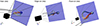 |
Fig. 3. Positions of the virtual spacecraft and their respective viewing fields. The black cube represents the spacecraft, while the violet area illustrates the field of view. Some representative lines of sight are included. |
Observer geometry and parameter combinations in the simulation setup.
3. Simulation results and discussion
We investigate the impact of different CME configurations and energy injection spectra on the resulting GS emission. Two CME setups were considered, classified by the ζ-parameter with values 30 and 70, and each is paired with injected electron energy distributions of spectral index δ = 2 and δ = 3. This section refers to individual cases by their respective ζ- and initial δ-values. However, the actual spectral indices of the electron populations vary over time and location due to transport effects, such as adiabatic cooling, particle losses, and scattering.
We begin by outlining the general features shared across all computed radio spectra and how they compare to real observations of type IV bursts. All obtained radio spectra (Figs. 4 and 5) exhibit a similar structure, containing a high-intensity centre surrounded by weaker emission. This feature is more pronounced in the δ = 2 cases compared to those with δ = 3. Similar intensity structures are regularly observed in dynamic spectra of type IV bursts, as illustrated in Fig. 1 and documented by studies such as Melnik et al. (2018), Vasanth et al. (2019), Morosan et al. (2020), and Kumari (2022). The high-intensity cores in our simulations emerge from the solution due to the local electron distribution, the CME magnetic field strength, and the viewing geometry (see paragraphs below). Broadband features with locally spiky or burst-like enhancements are often associated with emission originating in the MFR flanks near the footpoints, where magnetic field strengths are high and pitch-angle anisotropies are pronounced. These conditions are entirely consistent with the GS framework.
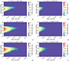 |
Fig. 4. Synthetic radio spectra for the CME case with ζ = 30. The panels in the left column show the observed radio emission from the injection spectrum with δ = 2 seen from the three spacecraft locations, while the panels in the right column contain the radio emission from the injection spectrum with δ = 3. |
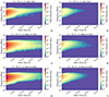 |
Fig. 5. Synthetic radio spectra for the CME case with ζ = 70. The panels in the left column show the observed radio emission from the injection spectrum with δ = 2 seen from the three spacecraft locations, while the panels in the right column contain the radio emission from the injection spectrum with δ = 3. |
Furthermore, all twelve spectra exhibit a drift of the intensity peak from higher to lower frequencies over time, resulting in broad, upward-drifting emission lanes in the time-frequency domain (with the frequency axis being inverted in the plots). This behaviour is typical for synchrotron emission from electrons in the energy range of 1–10 MeV in expanding, twisted MFRs, such as the Titov–Démoulin model used in our simulations, where the internal magnetic field weakens with time. Since the synchrotron peak frequency scales approximately with the square of the magnetic field strength (νpeak ∝ B2), this leads to a downward shift in frequency as the CME evolves. This effect is reinforced by the adiabatic cooling of electrons, which reduces their energy as they propagate. To quantify this behaviour, Table 2 lists estimated drift rates (in MHz/s) for all twelve spectra shown in Figs. 4 and 5. Drift rates were obtained by applying a linear fit to the time evolution of the intensity peaks over the first ∼30 min (in order to compare across all cases). While no clear trend emerges across all cases, we find that the halo-view configuration consistently exhibits the strongest negative drift rates.
Frequency drifts in type IV spectra, especially those associated with CMEs, have been frequently reported across a broad range of values. For instance, Kumari et al. (2021) identified downward frequency drifts in the majority of CMEs in their sample, using drift rates (in absolute value) |Rdrift|≥0.03 MHz/s as an indicator for IVm bursts. The authors found that most type IV bursts exhibited drift rates |Rdrift|≤0.5 MHz/s. Other studies report higher drift rates for fine structures embedded within type IV continua, ranging from several MHz/s up to tens of MHz/s (Nishimura et al. 2013; Melnik et al. 2018), while the background continuum typically drifts more slowly, with |Rdrift|≈10 kHz/s (Melnik et al. 2018). In this context, the drift rates obtained from our simulations fall towards the lower end of the reported literature values. A plausible explanation may lie in our modelling framework including only synchrotron/GS emission, where frequency drifts primarily arise from the gradual weakening of the magnetic field within the expanding MFR. It should be further noted that the reported drift rates were mostly derived at lower frequencies compared to our results, which may additionally explain discrepancies.
The GS emission is detected at all spacecraft positions from the time of electron injection (approximately 30 min into the simulation, with t = 0 min being the time of CME eruption), as the CME is initially entirely within the field of view. In general, the radio bursts are obtained in frequency ranges between 20 MHz and 8 GHz, with core intensities > 10−4 sfu (solar flux units) and < 103 sfu (see peak intensities in Table 2), and durations between ∼30 min and ∼2 h.
Frequency drift rates, Rdrift, estimated over the first ∼30 minutes after electron injection, and peak intensities for the different simulation configurations.
While type IV bursts are commonly detected in the 101–102 MHz range (Melnik et al. 2018; Vasanth et al. 2019; Morosan et al. 2020; Kumari et al. 2021; Kumari 2022; Mohan et al. 2024), observations also show extensions to higher frequencies from 102–103 MHz (Liu et al. 2018; Morosan et al. 2019) to several 103 MHz (Xie et al. 2002; Nishimura et al. 2013; Karlický & Rybák 2020). Similarly, reported spectral flux densities span a wide range, from 101–102 sfu (Dulk 1973; Carley et al. 2017; Melnik et al. 2018) over multiple 102 sfu (Bouratzis et al. 2015) to around 103 sfu (Melnik et al. 2018), and even approaching 104 sfu in cases involving fine structures (Alissandrakis et al. 2019). It is important to note that the peak intensities also depend on the number of injected electrons. Finally, recorded type IV durations are also highly variable, ranging from a few minutes (Karlický & Rybák 2020; Morosan et al. 2021; Kumari et al. 2021; Mohan et al. 2024) to several hours (Liu et al. 2018; Melnik et al. 2018; Vasanth et al. 2019). Historically, type IVm were associated with durations < 1 h, while durations > 1 h were attributed to type IVs. However, more recent studies report IVm events lasting > 1.5 h (Ramesh et al. 2013) and even > 2.5 h (Vasanth et al. 2019; see also the discussion in Kumari et al. 2021). These comparisons suggest that our synthetic GS spectra are physically realistic in terms of frequency range, spectral flux density, and duration.
When comparing the intensities for different spectral indices of the injected electrons at each spacecraft location, we consistently find higher intensities and longer radio burst durations for δ = 2 compared to δ = 3. This outcome is expected, as the spectrum with δ = 2 is flatter than that with δ = 3, meaning a larger fraction of the electron population is in the high-energy range. Consequently, the GS spectrum is dominated by higher-energy electrons, which produce stronger emission due to their greater radiative power (see Liénard formula or Eq. (2)). We further note that, due to the energy dependence of particle transport, the intensity ratios between these two cases are not constant over time. The case with initial δ = 2 not only contains more electrons of higher energy, but also a greater fraction of faster particles, yielding different transport behaviour over time and leading to distinct evolution of the injection spectra.
Next, we analyse the individual CME cases. Figure 4 presents the radio spectra obtained for the case ζ = 30, with δ = 2 in the left column and δ = 3 in the right column. The spectra are shown from the point of particle injection up to about 2.5 hours into the simulation. Considering the left column (δ = 2), at the first spacecraft position, where the observer is directly ahead of the CME, we find a peak intensity ratio of approximately Imax, δ = 2/Imax, δ = 3 ≈ 1100. At the second spacecraft location (observer viewing the MFR edge-on), the ratio is about 564. A similar ratio (roughly 560) is observed when the observer is directly above the CME (face-on view). The results are qualitatively similar for the δ = 3 cases in the right column (see Table 3).
Peak intensity ratios across observer positions, spectral indices, and CME cases.
The synthetic GS emission across different spacecraft positions also reveals noteworthy differences. Comparison of peak intensities between the edge-on and halo view for ζ = 30 and δ = 2 (panels a and c in Fig. 4) indicates a ratio of Imax, edge − on/Imax, halo ≈ 13. In contrast, a comparison between the face-on and halo view (panels a and e) yields Imax, face − on/Imax, halo ≈ 23, highlighting the strong variation in GS intensity with observer vantage point.
The variation in the radio emission spectra across the three observer positions can be understood in terms of the local magnetic field strength and the viewing angle. The GS emission is sensitive to the observer’s viewpoint relative to the MFR geometry. The GS brightness is proportional to the component of the magnetic field perpendicular to the electron motion, given by the electron pitch-angle, as B⊥ = B sin α. Thus, the viewing angle has a strong influence on both the emission intensity and the visibility of frequency drift.
The halo view aligns the observer’s LOS with the magnetic field lines that are essentially approximately parallel to the viewing direction, particularly along the MFR flanks. The field lines become more perpendicular only closer to the CME apex. Because GS emission is strongest when the magnetic field is perpendicular to the LOS, this geometry results in weaker overall emission, although the frequency drift remains visible.
From the edge-on view, the observer’s LOS traverse both CME flanks, encountering a thicker cross-section of the MFR where magnetic fields are both stronger and more perpendicular to the LOS. This configuration enhances the GS brightness and supports magnetic mirroring, as the magnetic field converges near the anchored MFR footpoints, which remain part of the closed field structure and exhibit the highest magnetic field strengths in the simulation. These conditions enable effective particle trapping and sustained GS emission.
Finally, the face-on view provides visibility of both CME flanks and part of the apex, with many LOS quasi-perpendicular to the flux rope axis. This geometry yields the strongest GS emission of the three configurations, owing to both favourable pitch-angle orientation and a large effective emitting region. Again, qualitatively similar results were obtained for the simulations with spectral index δ = 3 (see Table 3). It is worth noting that these results are specific to the generated MFR configuration. Increasing the twist of the MFR would modify the magnetic field geometry, change local viewing angles, and thus modify the observed GS emission.
Figure 5 shows the radio spectra obtained from the COCONUT simulation with the CME of ζ = 70. The plots are arranged similarly to those in Fig. 4, that is, the left column presents results based on spectral index δ = 2, while the right column shows the plots for δ = 3. Comparing the results for different spectral indices and spacecraft positions, we find qualitatively the same trends as in the CME case ζ = 30. Again considering the δ = 2 spectrum, we find that, for the halo view, the ratio between the peak intensities for the two spectral indices is approximately Imax, δ = 2/Imax, δ = 3 ≈ 620. At the edge-on-view location, we find a ratio of approximately 310, while at the face-on-view position, a ratio of about 208 is observed. The δ = 3 electron spectrum results are qualitatively similar (see Table 3). The differences across observer positions again indicate that from the face-on-view vantage point, the highest intensity is detected, followed by the edge-on-view and halo-view positions. The ratios between the peak intensities are Imax, edge − on/Imax, halo ≈ 7.2 and Imax, face − on/Imax, halo ≈ 12.8.
In the ζ = 70 case, our simulations additionally reveal a secondary emission lane at higher frequencies, distinct in drift rate and typically weaker than the main lane. These secondary lanes appear only in the edge-on and face-on view configurations, where some of the LOS from the observer’s viewing field intersect regions in the lower MFR flanks close to the MFR footpoints. Although the actual footpoints are not directly visible in these views, the detected GS emission originates from nearby locations where the magnetic field is strong, and the LOS orientation is largely perpendicular to the local field direction. These regions also exhibit enhanced pitch-angle anisotropies and may contain distinct populations of high-energy electrons. The footpoints themselves remain anchored and largely static; however, the close MFR flank regions continue to expand over time, leading to moderate field weakening and a slight frequency drift. As electrons move into stronger magnetic fields near the footpoint regions, they conserve their magnetic moment μm = p⊥2/(2 me B) with perpendicular momentum component p⊥, requiring an increase in pitch-angle and leading to magnetic mirroring. This process results in localised, time-varying enhancements in GS brightness that manifest as the observed secondary emission lanes.
The total synchrotron power from a single relativistic electron can be derived from the Liénard formula (Rybicki & Lightman 1986), and is approximately given by
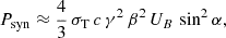 (2)
(2)
where the emission strength depends on the electron speed, the magnetic energy density UB = B2/(8 π), and the pitch-angle term sin2α. Here, σT denotes the Thomson scattering cross-section, c the speed of light in vacuum, and β = v/c. Near the MFR footpoints, both B and α tend to be large, substantially enhancing Psyn. As electrons are trapped within the MFR, they mirror at the stronger magnetic fields near the footpoints and travel back toward the weaker field near the MFR apex. Each time they pass through the footpoint regions, they produce bursts of local synchrotron emission, leading to a periodic emission pattern. Since the lower MFR regions near the magnetic footpoints are compact and maintain strong magnetic fields and large pitch angles, they produce locally strong GS emission despite their limited spatial extent. In our simulation setup, electrons are magnetically confined and mirror in these lower regions of the MFR, which remain anchored to the surface. This trapping mechanism contributes to the intermittent GS enhancements observed along the LOS intersecting these regions.
In contrast, the primary GS lane originating from the expanding MFR’s main body appears smoother and more continuous. The gradual expansion of the MFR causes the magnetic field magnitude to decrease, leading to a steady, upward frequency drift. Although magnetic fields near the footpoints are stronger, the total emission is dominated by the larger electron population distributed throughout the main body of the flux rope. The secondary emission lane, by comparison, appears more intermittent and consists of faint, locally enhanced features of GS emission. These features arise from a smaller electron population and are linked to confined mirroring in lower regions of the MFR flanks near the footpoints.
In more complex scenarios, flux ropes can expand rapidly and non-ideally, in the solar corona developing kinks, deflections, and asymmetries. These deformations may produce multiple distinct drifting GS lanes, each dependent on observer perspective and characterised by unique emission signatures. While our model assumes a simplified scenario with constant footpoints and no new flux emergence or footpoint diffusion, more intricate flux rope dynamics, such as increased twist or enhanced poloidal magnetic fields, could introduce localised gradients that might alter electron mirroring. In such cases, bursty broadband emissions can arise near footpoints and throughout other regions of the flux rope structure.
We note that the employed MFR model is already significantly more realistic than many idealised models historically used in GS studies (e.g. Dulk 1973; Fleishman & Melnikov 2003; Kuznetsov et al. 2015). Our erupting MFR introduces a dynamically evolving magnetic topology with strong twist, leading to varying field curvatures and strengths, all of which directly affect particle transport and confinement. Furthermore, the continued expansion and radial outward propagation of the MFR also involves time-dependent variations in both field strength and geometry, capturing important physical aspects relevant to GS emission in type IV bursts. In contrast, flux emergence and footpoint diffusion processes occur on much longer timescales (e.g. Giacalone & Jokipii 2004) than those associated with the particle acceleration and GS emission that we modelled here in the low corona, and are therefore expected to have a negligible influence on the simulation results.
Finally, we compare the differences in the intensities of the GS emission for the different CME cases. Considering the spectral index δ = 2, we note from the halo view perspective that the peak intensity in the ζ = 70 case is about 16 times higher compared to ζ = 30, at the edge-on view about 9 times higher, and at the face-on view also about 9 times higher. Qualitatively similar results are found for the δ = 3 spectra, and all ratios are summarised in Table 3. The stronger GS intensities in the ζ = 70 simulation can be attributed to the stronger magnetic field strengths present within the CME, consistent with Eq. (2). Additionally, a higher degree of twist associated with larger ζ-values may enhance the variation in the magnetic field along the MFR, promoting more effective magnetic mirroring and particle confinement, thus yielding longer-lasting and more intense GS emission.
To further illustrate differences in the observed GS emission intensities and their relationship to the magnetic field configuration, Fig. 6 shows the weighted mean magnetic field strength evolution for different observer vantage points and CME setups. The mean field was computed by weighting the magnetic field along each line of sight using the electron distribution from the δ = 2 case. The result was then averaged across all LOS for each observer position. These values are not direct measurements of the local field at emission sites, but rather effective field strengths contributing to the observed GS signal from each vantage point. As a result, they tend to be lower than typical observational estimates (e.g. Maia et al. 2007; Tun & Vourlidas 2013), which often reflect localised peak values near the emission core. In our model, localised fields in parts of the CME (e.g. in the MFR flanks) are indeed higher, but their contribution is diluted in the averaged LOS-weighted magnetic field.
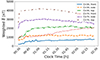 |
Fig. 6. Comparing the weighted mean magnetic field strength over time for different observer positions and CME cases. For calculating the weighted average, |

A clear positive correlation is observed between stronger magnetic fields and higher GS emission intensities. The highest emission levels occur in the ζ = 70 CME simulation for the face-on and edge-on views, which coincide with the strongest weighted magnetic fields shown in Fig. 6. Additionally, the halo view observer in the ζ = 70 case registers stronger magnetic fields than the halo and edge-on view observers in the ζ = 30 simulation, consistent with the observed peak GS intensities (see also Fig. 8).
The magnetic fields observed in the ζ = 70 halo view are initially weaker than those in the ζ = 30 face-on view, which is consistent with the detection of slightly lower GS intensities; this trend, however, reverses at later times. Notably, the rising trend of the ζ = 70 halo view curve does not necessarily indicate an increase in the CME’s field strength but may instead result from CME expansion. When comparing field strengths along individual halo view LOS, we observe that increasing values occur along LOS farther from 90° colatitude and 180° longitude (i.e. the central launch coordinates of the CME) and into which the CME expands. In contrast, LOS already intersecting the CME and closer to these coordinates show a declining field strength over time. As a result, the final curve in Fig. 6 reflects the growing influence of oblique LOS contributing to the overall averaging.
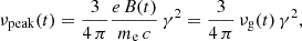
As described earlier, the simulations both in Figs. 4 and 5 indicate a shift of the peak intensities from higher to lower frequencies with time. To illustrate this frequency drift, we present two examples in Fig. 7, where the left panel shows the case ζ = 30 (same as the top left panel in Fig. 4), and the right panel shows the case ζ = 70 (same as the top left panel in Fig. 5). Both panels correspond to the halo view and are based on δ = 2. The black dotted curve indicates the peak intensities in the observed radio spectrum at each time step. To compare the results with theoretical expectations and to serve as a form of model validation, we additionally calculated the characteristic synchrotron peak frequencies following Ginzburg (1979) and Longair (1992) as
 (3)
(3)
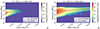 |
Fig. 7. Radio spectra with the peak intensity drifts from the simulation results and those calculated from theory. Exemplary, the drift of the peak intensity from higher to lower frequencies with time is shown for the case ζ = 30, δ = 2 (left panel), and ζ = 70, δ = 2 (right panel), both seen from the halo view. The black dotted curve shows the peak intensities from the simulation results, while the dark-red dashed curve shows the theoretical peak intensities calculated with Eq. (3). |
which are included as dark-red dashed curves in Fig 7. For the magnetic field in Eq. (3), we calculated a linearly weighted mean of B along each line of sight, using normalised particle intensities as weights. The simulation and theoretical peak frequencies are in reasonable agreement, showing a similar trend. We note that Eq. (3) is formulated for a single (constant) Lorentz factor. Since the highest-energy electrons contribute most to the GS emission in type IV radio bursts, we computed the Lorentz factor based on an electron kinetic energy of 9 MeV. However, choosing lower energies can significantly alter the theoretical curve, as the Lorentz factor in Eq. (3) is a constant scaling factor. For instance, using a kinetic energy of 6 MeV instead of 9 MeV would reduce the theoretical frequencies to approximately 47% of their original values.
Finally, we illustrate in Fig. 8 single-line profiles of the observed intensities as a function of frequency, approximately 32 minutes into the simulation and about 3 minutes after the electron injection. The left column shows ζ = 30 results, while the right column corresponds to ζ = 70, with rows ordered according to the three spacecraft positions. Each panel contains results based on the two spectral indices δ = 2 (black solid curve) and δ = 3 (red dashed curve). As noted in the discussion of the histograms above, the smaller spectral index (i.e. a flatter slope) consistently produced higher intensities.
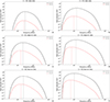 |
Fig. 8. Intensity curves as a function of frequency for a single time. The panels in the left column show the emission spectra in the case ζ = 30 of the electrons injected with spectral indices δ = 2 (black solid line) and δ = 3 (red dashed line). In contrast, the right column depicts the equivalent results in the case ζ = 70. Vertical lines mark the roll-over (or peak) frequencies. All spectra were recorded approximately 32 minutes into the simulation, which is about 3 minutes after the injection of the electrons. |
Furthermore, in all cases, the roll-over (i.e. the transition from the optically thick, self-absorbed regime to the optically thin, emission-dominated regime), indicated by the vertical lines, occurs at higher frequencies for the δ = 2 electron spectrum compared to the δ = 3 spectrum. The roll-overs are found between 165 MHz and 300 MHz in the ζ = 30 simulation, and between 65 MHz and 145 MHz in the ζ = 70 simulation, with those for the smaller spectral index being shifted to higher frequencies by approximately 40–70 MHz.
Comparing the spectra across the spacecraft positions for each CME case also reveals a shift of the roll-over frequency to lower values for vantage points where stronger GS emission was observed. When comparing the results across the two CME cases, we find that for ζ = 70 (a stronger magnetic field), the roll-over occurs at lower frequencies (approximately 65–145 MHz) compared to the corresponding ζ = 30 case (approximately 165–300 MHz).
At first glance, this contradicts Eq. (3), since the frequency at the intensity peak scales with the electron gyrofrequency and thus with the magnetic field strength. However, the spectra in Fig. 8 show that the slopes of the intensity curves in the ζ = 70 case are steeper than in the ζ = 30 case, suggesting stronger self-absorption, which shifts the roll-over to lower frequencies, reducing the transition to the optically thin regime.
Although the intensity curves displayed in Fig. 8 do not have a clear power-law form, they nonetheless suggest spectral indices χ that are steeper than those predicted by conventional analytical models of synchrotron and GS emission. In the optically thin regime, the typical relation for synchrotron emission is  (Ginzburg & Syrovatskii 1964), while a commonly used approximation for GS emission is
  (Dulk & Marsh 1982). As expected, the GS slope is steeper than that of pure synchrotron emission, likely due to propagation effects and the influence of the ambient medium. At the same time, these idealised expressions do not fully capture the complexities of real systems. Observational data frequently reveal significantly steeper indices, and our particle transport simulations are consistent with this pattern, showing early deviations from the initial spectral index of the injected electron distributions towards steeper slopes. This steepening may, in part, be explained by energy-dependent transport effects. Lower-energy electrons (e.g. ∼100 keV) have longer effective residence times in the flux rope due to their smaller velocities and reduced mirroring rates. In contrast, higher-energy electrons undergo more frequent magnetic mirroring between footpoints, increasing their probability of entering the loss cone and precipitating. Thus, their reduced contribution to the observed emission can lead to a steeper spectral slope. Additional discrepancies between analytical predictions and our numerical results may arise from uncertainties in the ambient plasma properties and simplifications inherent in analytical models.
While we considered only (incoherent) GS emission in this work, the presence of coherent emission mechanisms, often proposed for type IV bursts, cannot be ruled out. Plasma emission, in particular, has been suggested for both type IVs (Weiss 1963; Benz & Tarnstrom 1976) and type IVm bursts (Gary et al. 1985; Morosan et al. 2019). In addition, maser emission driven by a maser instability in nonthermal electron populations with strong perpendicular anisotropy, typically characterised by a loss-cone distribution, has frequently been proposed as a contributing mechanism (Winglee & Dulk 1986; Aschwanden & Benz 1988; Treumann et al. 2011; Morosan et al. 2016). Under suitable conditions, such instabilities can amplify electromagnetic waves near the electron gyrofrequency (e.g. Tsytovich 1970; Papadopoulos & Freund 1979; Galeev & Krasnoselskikh 1979). Whether such plasma instabilities actually develop in coronal conditions similar to those modelled here, and whether the resulting coherent emission is present in observed type IV radio spectra, remains an open and debated question (e.g. Morosan et al. 2016; Carley et al. 2017).
4. Summary and conclusions
In this study, we have presented a novel coupling of three models to generate synthetic radio spectra and investigate the influence of different injection spectra and initial CME parameters on the observed emission spectra. Using the 3D MHD coronal model COCONUT, we constructed a coronal configuration based on an HMI magnetogram. We then performed two simulations, each modelling a CME as an MFR with different initial properties in terms of magnetic field strength and speed, encapsulated in the dimensionless parameter ζ, here with values of 30 and 70. Next, we used the SEP model PARADISE to simulate energetic electrons trapped within the erupting MFR. Finally, using COCONUT’s plasma parameters and the electron energy distributions obtained from PARADISE, we applied the UFGSCs to compute GS emission from the trapped electron populations as observed from three different vantage points (halo view, edge-on view, face-on view) in the solar corona.
Comparing the radio spectra for each CME across different spectral indices, we found that the flatter spectrum with δ = 2 consistently produced stronger GS radiation and longer-lasting radio bursts than the steeper spectrum with δ = 3. A comparison between the two CMEs revealed that the electrons in the ζ = 70 CME, characterised by a stronger initial magnetic field strength (nearly twice that of the ζ = 30 CME) and a higher initial speed, generated much more intense GS emission. Finally, comparing the three observer positions against each other demonstrated that the strongest GS emission was detected when the spacecraft was above the CME, followed by the perspective viewing both CME flanks from edge-on. In contrast, the weakest GS emission was detected when the observer faced the front of the approaching CME (halo view).
It should be noted that modifying the employed energy range or further steepening the injection spectrum would significantly affect the resulting GS emission, including frequency range, intensity, and duration. Since an electron’s pitch angle directly influences its radiated power, the initial pitch-angle distribution of the injected population can also impact the morphology and quantitative properties of the resulting type IV spectra. While we adopted an isotropic distribution in this study, test simulations with highly beamed electron populations revealed a range of pitch-angle distributions at early times in the type IV event, depending on the energy channel and location. For instance, we found single electron beams (both field and anti-field aligned), counter-beam populations, and populations transitioning towards isotropy. The computed spectra were morphologically similar, but showed slightly reduced peak intensities (by ∼20%). This is consistent with theoretical expectations for smaller pitch angles. Furthermore, the reduced GS emission may also stem from a significant fraction of particles entering the magnetic bottle’s loss cone, leading to precipitation into the inner simulation boundary and their removal from the simulation.
A detailed exploration of these dependencies goes beyond the scope of the present study. In future work, we aim to conduct MHD and transport simulations with significantly higher temporal resolution (e.g. 10 s sampling times), focusing on the early evolution (first ∼30–60 min) of type IV events to investigate the role of pitch-angle and other energy distributions (e.g. initially monoenergetic or kappa-distributed, or using different energy ranges) more systematically.
The radio spectra obtained from our simulations suggest that type IV radio bursts contain GS radiation from electrons trapped within the strong magnetic field lines of CMEs. Furthermore, our results indicate that the GS emission primarily originates from the CME flanks, consistent with imaging observations and previous studies (see, e.g. Gopalswamy & Kundu 1990; Bastian et al. 2001; Bain et al. 2014; Carley et al. 2020). Additionally, our simulations demonstrate that the orientation of the flux rope relative to the observer’s LOS significantly influences the detected emission (e.g. Nindos 2020). This finding highlights the importance of multi-messenger observations, as the evolution of the radio source cannot be fully understood without complementary observational constraints.
All computed emission spectra exhibit a similar structure, consisting of a high-intensity core surrounded by regions of weaker emission, with the peak intensity gradually drifting to lower frequencies over time. These spectral features are physical within the GS framework implemented in the UFGSCs and arise entirely from incoherent GS emission. The spatial and spectral variations, such as LOS-dependent intensity patterns and secondary emission lanes, can be consistently understood using the Liénard formula (Schwinger 1949). GS emission is particularly enhanced in MFR flank regions near the footpoints, where the local pitch-angle distribution and magnetic field geometry favour spiky, burst-like signatures. These regions naturally support GS radiation, as similar behaviour is expected whenever electrons are injected into an MFR, though the absolute brightness depends on the flux rope structure itself.
While the present work did not attempt a case study, several aspects support the physical realism of our simulation results. All three coupled models are physics based, providing physical credibility beyond empirical parameter fitting. Moreover, the morphological features of the obtained spectra match type IV observations. Finally, our results quantitatively fall within observationally established ranges in terms of frequency intervals, spectral flux densities, frequency drift rates (supported both by literature values and theoretical expectations), and event durations.
In conclusion, our simulation results yield several key insights regarding GS emission in type IV radio bursts:
-
A synchrotron and GS background is likely present in most type IV radio bursts. The brightness of this background is determined by the high-energy electron distribution, the magnetic field strength, the topology, and other properties of the MFR confining the electrons, as well as its orientation relative to the observer.
-
GS emission is strongest in the CME flanks near the footpoints rather than the CME apex, due to stronger magnetic field strengths and more favourable pitch-angle distributions, supporting earlier observations of enhanced GS emission from CME flanks.
-
Both spectral and spatial drift are natural consequences of CME expansion and evolving field conditions. In our simulations, the GS emission source (i.e. energetic electrons) moves outwards with the expanding MFR, while the associated spectral drift depends on the magnetic field evolution and energetic electron distribution. This may help explain why some type IV bursts are observed as moving, while others seem stationary in radio imaging.
These findings emphasise the importance of considering GS emission as a fundamental mechanism in type IV radio bursts, and illustrate how CME properties and observer geometry shape the observed radio spectra. Additionally, our results suggest that type IVm spectra can exhibit drift rates below thresholds proposed in previous studies (e.g. Kumari et al. 2021), implying that some bursts classified as IVs might still be associated with erupting MFRs. While our analysis is solely based on incoherent GS radiation, it does not necessarily exclude the presence of other emission mechanisms, which may contribute or modify the observed spectral features. In particular, the observed spectral flux densities may result from a superposition of multiple mechanisms, including coherent processes, which may yield stronger emission than the GS component alone in our simulations. Ultimately, this study helps clarify the role of GS emission in shaping radio spectra and provides a framework for identifying regions where additional coherent emission from the maser instability might occur, which is beyond the scope of this work.
The present study provides a foundation for future research on CME kinematics and GS emission to infer electron properties and magnetic field characteristics within CMEs, with the potential for direct validation using PSP’s radio and particle measurements. Future work will also explore magnetoionic properties of GS radiation. In particular, we will focus on polarisation to refine estimates of magnetic field strength and topology.
Hereafter, we refer to the MFR as the CME.
Acknowledgments
We thank the anonymous referee for their valuable comments, which helped improve the clarity and rigour of the manuscript. Computational resources and services used in this work were provided by the VSC (Flemish Supercomputer Center), funded by the Research Foundation – Flanders (FWO) and the Flemish Government – department EWI. E.H. is grateful to the Space Weather Awareness Training Network (SWATNet) funded by the European Union’s Horizon 2020 research and innovation program under the Marie Skłodowska-Curie grant agreement No. 955620. N.W. acknowledges funding from the KU Leuven project 3E241013. I.C.J. is grateful for support by the Research Council of Finland (SHOCKSEE, grant No. 346902, and X-Scale, grant No. 371569), and the European Union’s (E.U’s) Horizon 2020 research and innovation program under grant agreement No. 101134999 (SOLER). A.V. is supported by NASA grant 80NSSC21K1860. S.P. is funded by the European Union. Views and opinions expressed are, however, those of the author(s) only and do not necessarily reflect those of the European Union or ERCEA. Neither the European Union nor the granting authority can be held responsible for them. This project (Open SESAME) has received funding under the Horizon Europe programme (ERC-AdG agreement No 101141362). These results were also obtained in the framework of the projects C16/24/010 C1 project Internal Funds KU Leuven), G0B5823N and G002523N (WEAVE) (FWO-Vlaanderen), and 4000145223 (SIDC Data Exploitation (SIDEX2), ESA Prodex).
References
- Agueda, N., & Vainio, R. 2013, J. Space Weather Space Clim., 3, A10 [NASA ADS] [CrossRef] [EDP Sciences] [Google Scholar]
- Alissandrakis, C. E., Bouratzis, C., & Hillaris, A. 2019, A&A, 627, A133 [NASA ADS] [CrossRef] [EDP Sciences] [Google Scholar]
- Alissandrakis, C. E., Nindos, A., Patsourakos, S., & Hillaris, A. 2021, A&A, 654, A112 [NASA ADS] [CrossRef] [EDP Sciences] [Google Scholar]
- Aschwanden, M. J., & Benz, A. O. 1988, ApJ, 332, 466 [NASA ADS] [CrossRef] [Google Scholar]
- Bain, H. M., Krucker, S., Saint-Hilaire, P., & Raftery, C. L. 2014, ApJ, 782, 43 [Google Scholar]
- Baratashvili, T., Brchnelova, M., Linan, L., Lani, a., & Poedts, S. 2024, A&A, 690, A184 [NASA ADS] [CrossRef] [EDP Sciences] [Google Scholar]
- Bastian, T. S., Pick, M., Kerdraon, A., Maia, D., & Vourlidas, A. 2001, ApJ, 558, L65 [Google Scholar]
- Benz, A. O., & Tarnstrom, G. L. 1976, ApJ, 204, 597 [CrossRef] [Google Scholar]
- Born, M., & Wolf, E. 1959, Principles of Optics Electromagnetic Theory of Propagation, Interference and Diffraction of Light (New York: Pergamon Press) [Google Scholar]
- Bouratzis, C., Hillaris, A., Alissandrakis, C. E., et al. 2015, Sol. Phys., 290, 219 [NASA ADS] [CrossRef] [Google Scholar]
- Brchnelova, M., Zhang, F., Leitner, P., et al. 2022, J. Plasma Phys., 88, 905880205 [NASA ADS] [CrossRef] [Google Scholar]
- Carley, E. P., Vilmer, N., Simões, P. J. A., & Fearraigh, B. O. 2017, A&A, 608, A137 [NASA ADS] [CrossRef] [EDP Sciences] [Google Scholar]
- Carley, E. P., Vilmer, N., & Vourlidas, A. 2020, Front. Astron. Space Sci., 7, 79 [Google Scholar]
- Chernov, G. P. 2006, Space Sci. Rev., 127, 195 [Google Scholar]
- Dulk, G. A. 1973, Sol. Phys., 32, 491 [Google Scholar]
- Dulk, G. A. 1985, ARA&A, 23, 169 [Google Scholar]
- Dulk, G. A., & Marsh, K. A. 1982, ApJ, 259, 350 [NASA ADS] [CrossRef] [Google Scholar]
- Fleishman, G. D., & Kuznetsov, A. A. 2010, ApJ, 721, 1127 [NASA ADS] [CrossRef] [Google Scholar]
- Fleishman, G. D., & Melnikov, V. F. 2003, ApJ, 587, 823 [Google Scholar]
- Galeev, A. A., & Krasnoselskikh, V. V. 1979, Soviet. Astron. Lett., 5, 257 [Google Scholar]
- Galeev, A. A., Karpman, V. I., & Sagdeev, R. Z. 1965, Sov. Phys. Dokl., 9, 681 [Google Scholar]
- Gary, D. E., & Keller, C. U. (eds.) 2004, Solar and Space Weather Radiophysics (Dordrecht: Springer) [Google Scholar]
- Gary, D. E., Dulk, G. A., House, L. L., et al. 1985, A&A, 152, 42 [NASA ADS] [Google Scholar]
- Gergely, T. E. 1986, Sol. Phys., 104, 175 [Google Scholar]
- Giacalone, J., & Jokipii, J. R. 2004, ApJ, 616, 573 [NASA ADS] [CrossRef] [Google Scholar]
- Ginzburg, V. L. 1979, Theoretical Physics and Astrophysics (Oxford: Pergamon Press) [Google Scholar]
- Ginzburg, V. L., & Syrovatskii, S. I. 1964, The Origin of Cosmic Rays (Amsterdam: Elsevier) [Google Scholar]
- Gopalswamy, N., & Kundu, M. R. 1987, Sol. Phys., 114, 347 [NASA ADS] [CrossRef] [Google Scholar]
- Gopalswamy, N., & Kundu, M. R. 1990, Sol. Phys., 128, 377 [Google Scholar]
- Han Thanh, L., Scherer, K., & Fichtner, H. 2022, Phys. Plasmas, 29, 022901 [Google Scholar]
- Hariharan, K., Ramesh, R., Kathiravan, C., & Wang, T. J. 2016, Sol. Phys., 291, 1405 [Google Scholar]
- Howard, R. A., Michels, D. J., Sheeley, N. R., Jr, & Koomen, M. J. 1982, ApJ, 263, L101 [NASA ADS] [CrossRef] [Google Scholar]
- Husidic, E., Wijsen, N., Linan, L., et al. 2024, ApJ, 976, L31 [Google Scholar]
- Jebaraj, I. C., Kouloumvakos, A., Magdalenic, J., et al. 2021, A&A, 654, A64 [NASA ADS] [CrossRef] [EDP Sciences] [Google Scholar]
- Jebaraj, I. C., Kouloumvakos, A., Dresing, N., et al. 2023, A&A, 675, A27 [NASA ADS] [CrossRef] [EDP Sciences] [Google Scholar]
- Jebaraj, I. C., Agapitov, O. V., Gedalin, M., et al. 2024, ApJ, 976, L7 [NASA ADS] [CrossRef] [Google Scholar]
- Kansabanik, D., Mondal, S., & Oberoi, D. 2024, ApJ, 968, 55 [Google Scholar]
- Kaplan, S. A., & Tsytovich, V. N. 1969, Sov. Phys. Usp., 12, 42 [Google Scholar]
- Karlický, M., & Rybák, J. 2020, ApJS, 250, 31 [Google Scholar]
- Klein, K. L. 1987, A&A, 183, 341 [NASA ADS] [Google Scholar]
- Klein, K.-L., Musset, S., Vilmer, N., et al. 2022, A&A, 663, A173 [CrossRef] [EDP Sciences] [Google Scholar]
- Knock, S. A., & Cairns, I. H. 2005, J. Geophys. Res., 110, A01101 [Google Scholar]
- Kouloumvakos, A., Nindos, A., Valtonen, E., et al. 2015, A&A, 580, A80 [NASA ADS] [CrossRef] [EDP Sciences] [Google Scholar]
- Koval, A., Stanislavsky, A., Chen, Y., et al. 2016, ApJ, 826, 125 [NASA ADS] [CrossRef] [Google Scholar]
- Kumari, A. 2022, Sol. Phys., 297, 98 [NASA ADS] [CrossRef] [Google Scholar]
- Kumari, A., Morosan, D. E., & Kilpua, E. K. J. 2021, ApJ, 906, 79 [Google Scholar]
- Kundu, M. R. 1965, Solar Radio Astronomy (New York: Interscience Publication) [Google Scholar]
- Kuznetsov, A. A., & Fleishman, G. D. 2021, ApJ, 922, 103 [NASA ADS] [CrossRef] [Google Scholar]
- Kuznetsov, A. A., Van Doorsselaere, T., & Reznikova, V. E. 2015, Sol. Phys., 290, 1173 [CrossRef] [Google Scholar]
- le Roux, J. A., & Webb, G. M. 2009, ApJ, 693, 534 [Google Scholar]
- Linan, L., Regnault, F., Perri, B., et al. 2023, A&A, 675, A101 [NASA ADS] [CrossRef] [EDP Sciences] [Google Scholar]
- Litvak, A. G., & Trakhtengerts, V. Y. 1971, Soviet. J. Exp. Theor. Phys., 33, 921 [Google Scholar]
- Liu, H., Chen, Y., Cho, K., et al. 2018, Sol. Phys., 293, 58 [NASA ADS] [CrossRef] [Google Scholar]
- Longair, M. S. 1992, High Energy Astrophysics. Vol.1: Particles, Photons and their Detection, (Cambridge: Cambridge University Press) [Google Scholar]
- Lv, M., Chen, Y., Vasanth, V., et al. 2021, Sol. Phys., 296, 38 [Google Scholar]
- Maia, D. J. F., Gama, R., Mercier, C., et al. 2007, ApJ, 660, 874 [NASA ADS] [CrossRef] [Google Scholar]
- Maksimovic, M., Pierrard, V., & Riley, P. 1997, Geophys. Res. Lett., 24, 1151 [NASA ADS] [CrossRef] [Google Scholar]
- Melnik, V. N., Rucker, H. O., Konovalenko, A. A., et al. 2018, arXiv e-prints [arXiv:1802.06249] [Google Scholar]
- Melrose, D. B. 1968, Ap&SS, 2, 171 [Google Scholar]
- Melrose, D. B. 1980, Space Sci. Rev., 26, 3 [NASA ADS] [CrossRef] [Google Scholar]
- Melrose, D. B. 2017, Rev. Mod. Plasma Phys., 1, 5 [Google Scholar]
- Mohan, A., Mondal, S., Wedemeyer, S., & Gopalswamy, N. 2024, A&A, 686, A51 [NASA ADS] [CrossRef] [EDP Sciences] [Google Scholar]
- Mondal, S., Oberoi, D., & Vourlidas, A. 2020, ApJ, 893, 28 [NASA ADS] [CrossRef] [Google Scholar]
- Morosan, D. E., Zucca, P., Bloomfield, D. S., & Gallagher, P. T. 2016, A&A, 589, L8 [NASA ADS] [CrossRef] [EDP Sciences] [Google Scholar]
- Morosan, D. E., Kilpua, E. K. J., Carley, E. P., & Monstein, C. 2019, A&A, 623, A63 [NASA ADS] [CrossRef] [EDP Sciences] [Google Scholar]
- Morosan, D. E., Palmerio, E., Pomoell, J., et al. 2020, A&A, 635, A62 [NASA ADS] [CrossRef] [EDP Sciences] [Google Scholar]
- Morosan, D. E., Kumari, A., Kilpua, E. K. J., & Hamini, A. 2021, A&A, 647, L12 [NASA ADS] [CrossRef] [EDP Sciences] [Google Scholar]
- Nindos, A. 2020, Front. Astron. Space Sci., 7, 57 [NASA ADS] [CrossRef] [Google Scholar]
- Nishimura, Y., Ono, T., Tsuchiya, F., et al. 2013, Earth Planets Space, 65, 1555 [Google Scholar]
- Papadopoulos, K., & Freund, H. P. 1979, Space Sci. Rev., 24, 511 [Google Scholar]
- Perri, B., Leitner, P., Brchnelova, M., et al. 2022, ApJ, 936, 19 [NASA ADS] [CrossRef] [Google Scholar]
- Petrosian, V. 1981, ApJ, 251, 727 [Google Scholar]
- Pick, M., & Vilmer, N. 2008, A&ARv, 16, 1 [NASA ADS] [CrossRef] [Google Scholar]
- Ramaty, R. 1969, ApJ, 158, 753 [CrossRef] [Google Scholar]
- Ramesh, R., Kishore, P., Mulay, S. M., et al. 2013, ApJ, 778, 30 [NASA ADS] [CrossRef] [Google Scholar]
- Robinson, R. D. 1978, Sol. Phys., 60, 383 [CrossRef] [Google Scholar]
- Robinson, R. D., & Smerd, S. F. 1975, PASA, 2, 374 [Google Scholar]
- Rybicki, G. B., & Lightman, A. P. 1986, Radiative Processes in Astrophysics (Weinheim: Wiley-VCH) [Google Scholar]
- Salas-Matamoros, C., & Klein, K. L. 2020, A&A, 639, A102 [NASA ADS] [CrossRef] [EDP Sciences] [Google Scholar]
- Scherer, K., Fichtner, H., & Lazar, M. 2017, EPL (Europhysics Letters), 120, 50002 [Google Scholar]
- Schwenn, R., dal Lago, A., Huttunen, E., & Gonzalez, W. D. 2005, Ann. Geophys., 23, 1033 [Google Scholar]
- Schwinger, J. 1949, Phys. Rev., 75, 1912 [Google Scholar]
- Titov, V. S., & Démoulin, P. 1999, A&A, 351, 707 [NASA ADS] [Google Scholar]
- Titov, V. S., Török, T., Mikić, Z., & Linker, J. A. 2014, ApJ, 790, 163 [NASA ADS] [CrossRef] [Google Scholar]
- Treumann, R. A., Nakamura, R., & Baumjohann, W. 2011, Ann. Geophys., 29, 1673 [Google Scholar]
- Tsytovich, V. N. 1970, Nonlinear Effects in Plasma (New York: Springer) [Google Scholar]
- Tun, S. D., & Vourlidas, A. 2013, ApJ, 766, 130 [Google Scholar]
- van den Berg, J., Strauss, D. T., & Effenberger, F. 2020, Space Sci. Rev., 216, 146 [NASA ADS] [CrossRef] [Google Scholar]
- Vasanth, V., Chen, Y., Lv, M., et al. 2019, ApJ, 870, 30 [Google Scholar]
- Vourlidas, A. 2004, in Radio Observations of Coronal Mass Ejections, eds. D. E. Gary, & C. U. Keller (Dordrecht: Kluwer Academic Publishers), Astrophysics and Space Science Library, 314, 223 [Google Scholar]
- Vourlidas, A., Carley, E. P., & Vilmer, N. 2020, Front. Astron. Space Sci., 7, 79 [Google Scholar]
- Weiss, A. A. 1963, Aust. J. Phys., 16, 526 [NASA ADS] [CrossRef] [Google Scholar]
- Wijsen, N. 2020, Ph.D. dissertation, KU Leuven (Belgium) and Univ. Barcelona (Spain) [Google Scholar]
- Wijsen, N., Aran, A., Pomoell, J., & Poedts, S. 2019, A&A, 622, A28 [NASA ADS] [CrossRef] [EDP Sciences] [Google Scholar]
- Wilson, L. B., Mitchell, J. G., Szabo, A., et al. 2025, ApJ, 987, 31 [Google Scholar]
- Winglee, R. M., & Dulk, G. A. 1986, ApJ, 307, 808 [Google Scholar]
- Xie, R., Wang, M., Duan, C., et al. 2002, Sci. China A Math., 45, 97 [Google Scholar]
- Zheleznyakov, V. V. 1969, ApJ, 155, 1129 [Google Scholar]
- Zheleznyakov, V. V. 1970, Radio Emission of the Sun and Planets (New York: Interscience Publication) [Google Scholar]
- Zlotnik, E. Y., Zaitsev, V. V., Aurass, H., Mann, G., & Hofmann, A. 2003, A&A, 410, 1011 [NASA ADS] [CrossRef] [EDP Sciences] [Google Scholar]
Appendix A: Technical details of the numerical models
A.1. COCONUT
The coronal MHD model COCONUT solves the 3D ideal MHD equations to generate coronal configurations from 1 to 21.5 R⊙ (Perri et al. 2022). To model CMEs, we use the analytical modified Titov–Démoulin flux rope model (Titov & Démoulin 1999; Titov et al. 2014; Linan et al. 2023). An eruptive MFR is achieved by setting the ring current intensity I in the MFR to a value larger than the Shafranov intensity IS via
 (A.1)
(A.1)
which causes the magnetic pressure inside the MFR to exceed that of the ambient coronal plasma. In Eq. (A.1), ζ is a dimensionless parameter, R and a describe the major and minor radius of the flux rope, respectively, Bt is the toroidal magnetic field component, and Ii is a dimensionless variable that characterises the radial distribution of the poloidal magnetic field inside the MFR (for details, see Titov et al. 2014; Linan et al. 2023).
The initial placement of the CME footpoints (i.e. the locations where the MFR is magnetically anchored in the lower corona or photosphere) was around colatitude θ = 90° and Carrington longitude ϕ = 180°, with the centre of the toroidal axis located at a height d = 0.15 R⊙ above the solar surface. The minor radius was set to a = 0.1 R⊙, while the major radius was set to R = 0.3 R⊙. The unstructured COCONUT grid used about 1.5 million prism-shaped cells in concentric, radially expanding shells (see Brchnelova et al. 2022 for details). The output cadence of the MHD snapshots was about 87 seconds, and we used the first 2.5 hours of the COCONUT simulations for the subsequent particle transport simulations. We further note that the actual computational domain of COCONUT in our simulations extended to 25 R⊙, but we set the outer boundary in the subsequent particle transport simulations to 21.5 R⊙ to avoid any numerical outer boundary effects, following the recommendations by Brchnelova et al. (2022).
A.2. PARADISE
The particle transport code PARADISE solves the FTE in the present work in the form
 (A.2)
(A.2)
to derive spatio-temporal particle intensity distributions. In Eq. A.2, x is the spatial vector, and Dμμ is the pitch-angle diffusion coefficient. Detailed expressions for the individual terms in the FTE A.2 describing effects such as adiabatic cooling, focusing, and mirroring can be found, for instance, in Wijsen (2020) and le Roux & Webb (2009), while information about Dμμ can be found in Agueda & Vainio (2013).
To ensure robust statistics in the particle transport simulations, a total of 10.8 million electrons were injected in each simulation. While the pitch-angle diffusion coefficient is included in the FTE, for simplicity, we excluded cross-field (perpendicular) diffusion, and the guiding-centre drift velocity was set to zero, as it is expected to be negligible for electrons. The parallel mean free path length was fixed to λ∥ = 0.1 au. Further details about the coupling between COCONUT and PARADISE can be found in Husidic et al. (2024).
At each node along a line of sight and for each time step, the particle distribution function f, obtained from PARADISE, was passed to the UFGSCs as a 2D array fi, j = f(Ei, μj) in energy-pitch-angle space. Here, E denotes the kinetic energy, and f has the units cm−3 MeV−1. We added a background electron component to the PARADISE output to avoid exact zeros resulting from the logarithmic energy grid. This background was based on the relativistic regularised kappa distribution (rRKD; Han Thanh et al. 2022), reformulated in terms of relativistic kinetic energy  with electron rest mass m0, and provided in units cm−3 MeV−1. The local number density and temperature at a given time and position in the rRKD were extracted from the MHD simulation.
To ensure that the PARADISE electron distribution had physically meaningful units, we obtained the scaling factor by matching the injected particle distribution at 10 keV to the rRKD, parametrised by the local solar wind conditions obtained from the MHD simulation at the injection region and time. The influence of the background was minimised in all simulations by choosing κ = 8 and a cut-off parameter ξ = 0.001 for the rRKD (for details, see Scherer et al. 2017; Han Thanh et al. 2022). Figure A.1 shows the injected electron distribution (red solid curve) for δ = 2 and the background rRKD (blue dashed curve), demonstrating the scaling. As illustrated, the background distribution aligns with the PARADISE simulation at the lowest energy of the injection spectrum and remains below it across the whole energy range. Since the PARADISE distribution steepened during the transport simulation, selecting a κ-value of 8 ensured the background remained below the PARADISE distribution. This also helped to avoid excessively steep gradients in the total distribution, which could otherwise lead to numerical artefacts in the GS calculation and provide conditions resulting in occasional oversaturated pixels in the computed spectra, with intensities sometimes exceeding those of neighbouring pixels by several tens of orders of magnitude.
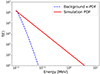 |
Fig. A.1. Comparing the distribution function tails of the background and the injected electron distribution. The particle distribution function (PDF) is plotted as a red solid graph, while the background rRKD with κ = 8 and ξ = 0.001 is plotted as a blue dashed graph. |
Including the background inevitably introduced a small GS contribution from it. However, due to the nonlinearity of the emission and absorption coefficients, the background contribution could not be directly subtracted. Nevertheless, simulations ran with the background distribution alone showed that subtracting its GS emission from that of the combined (PARADISE + background) distribution resulted in a change of less than 0.01% at the peak intensities.
All Tables
Frequency drift rates, Rdrift, estimated over the first ∼30 minutes after electron injection, and peak intensities for the different simulation configurations.
Peak intensity ratios across observer positions, spectral indices, and CME cases.
All Figures
|
Fig. 1. Dynamic radio spectrum of a type IV radio burst detected by the Sagamore Hill Solar Radio Observatory on 24 September 2011. Adapted from Kumari (2022). |
| In the text | |
|
Fig. 2. Illustration of the modelling chain for the generation of synthetic radio spectra. |
| In the text | |
|
Fig. 3. Positions of the virtual spacecraft and their respective viewing fields. The black cube represents the spacecraft, while the violet area illustrates the field of view. Some representative lines of sight are included. |
| In the text | |
|
Fig. 4. Synthetic radio spectra for the CME case with ζ = 30. The panels in the left column show the observed radio emission from the injection spectrum with δ = 2 seen from the three spacecraft locations, while the panels in the right column contain the radio emission from the injection spectrum with δ = 3. |
| In the text | |
|
Fig. 5. Synthetic radio spectra for the CME case with ζ = 70. The panels in the left column show the observed radio emission from the injection spectrum with δ = 2 seen from the three spacecraft locations, while the panels in the right column contain the radio emission from the injection spectrum with δ = 3. |
| In the text | |
|
Fig. 6. Comparing the weighted mean magnetic field strength over time for different observer positions and CME cases. For calculating the weighted average, |
| In the text | |
|
Fig. 7. Radio spectra with the peak intensity drifts from the simulation results and those calculated from theory. Exemplary, the drift of the peak intensity from higher to lower frequencies with time is shown for the case ζ = 30, δ = 2 (left panel), and ζ = 70, δ = 2 (right panel), both seen from the halo view. The black dotted curve shows the peak intensities from the simulation results, while the dark-red dashed curve shows the theoretical peak intensities calculated with Eq. (3). |
| In the text | |
|
Fig. 8. Intensity curves as a function of frequency for a single time. The panels in the left column show the emission spectra in the case ζ = 30 of the electrons injected with spectral indices δ = 2 (black solid line) and δ = 3 (red dashed line). In contrast, the right column depicts the equivalent results in the case ζ = 70. Vertical lines mark the roll-over (or peak) frequencies. All spectra were recorded approximately 32 minutes into the simulation, which is about 3 minutes after the injection of the electrons. |
| In the text | |
|
Fig. A.1. Comparing the distribution function tails of the background and the injected electron distribution. The particle distribution function (PDF) is plotted as a red solid graph, while the background rRKD with κ = 8 and ξ = 0.001 is plotted as a blue dashed graph. |
| In the text | |
Current usage metrics show cumulative count of Article Views (full-text article views including HTML views, PDF and ePub downloads, according to the available data) and Abstracts Views on Vision4Press platform.
Data correspond to usage on the plateform after 2015. The current usage metrics is available 48-96 hours after online publication and is updated daily on week days.
Initial download of the metrics may take a while.