| Issue |
A&A
Volume 701, September 2025
|
|
|---|---|---|
| Article Number | A39 | |
| Number of page(s) | 8 | |
| Section | Astrophysical processes | |
| DOI | https://doi.org/10.1051/0004-6361/202555574 | |
| Published online | 02 September 2025 | |
A double dipole geometry for PSR J0740+6620
1
Université de Strasbourg, CNRS, Observatoire astronomique de Strasbourg, UMR 7550, F-67000 Strasbourg, France
2
IRAP, CNRS, Université de Toulouse, CNES, 9 avenue du Colonel Roche, BP 44346, F-31028 Toulouse Cedex 4, France
3
LPC2E, OSUC, Univ Orléans, CNRS, CNES, Observatoire de Paris, F-45071 Orléans, France
4
ORN, Observatoire de Paris, Université PSL, Univ Orléans, CNRS, 18330 Nançay, France
⋆ Corresponding author: This email address is being protected from spambots. You need JavaScript enabled to view it.
Received:
19
May
2025
Accepted:
10
July
2025
Abstract
Context. Millisecond pulsars are known to show complex radio pulse profiles and polarisation position angle evolution with rotational phase. Small-scale surface magnetic fields and multipolar components are believed to be responsible for this complexity, due to the radiation mechanisms occurring close to the stellar surface but within the relatively small light cylinder compared to the stellar radius.
Aims. In this work, we use the latest NICER phase aligned thermal X-ray pulse profile of PSR J0740+6620 combined with radio and γ-ray pulse profiles and radio polarisation to deduce the best magnetic field configuration that can simultaneously reproduce the light curves in these respective bands.
Methods. We assumed a polar cap model for the radio emission and used the rotating vector model for the associated polarisation and a striped wind model for the γ-ray light curves, whereas we relied on the NICER collaboration results for the hot spot geometry.
Results. We demonstrate that an almost centred dipole can account for the hot spot location with a magnetic obliquity of α ≈ 51° and a line of sight inclination angle of ζ ≈ 82°. However, with this geometry, the hot spot areas are three times too large. We found a better solution consisting of two dipoles located just below the surface in approximately antipodal positions.
Conclusions. Our double dipole model is able to reproduce all the salient radio and γ-ray characteristics of PSR J0740+6620 including radio polarisation data. A double dipole solution is more flexible than an off-centred dipole because it has two independent magnetic axes and could hint at a magnetic field mostly concentrated within the crust and not in the core.
Key words: polarization / stars: magnetic field / pulsars: general / stars: rotation / pulsars: individual: PSR J0740+6620
© The Authors 2025
 Open Access article, published by EDP Sciences, under the terms of the Creative Commons Attribution License (https://creativecommons.org/licenses/by/4.0), which permits unrestricted use, distribution, and reproduction in any medium, provided the original work is properly cited.
This article is published in open access under the Subscribe to Open model. This email address is being protected from spambots. You need JavaScript enabled to view it. to support open access publication.
1. Introduction
Thanks to multi-wavelength observations of pulsar emission, a global picture of the neutron star magnetosphere and its radiation mechanisms is emerging. Whereas for non-recycled pulsars, the radio emission is well constrained to occur along dipolar magnetic field lines at several tens of stellar radii (Johnston et al. 2023), the γ-ray emission appears to emanate from the striped wind just beyond the light cylinder (Pétri & Mitra 2021) and the non-thermal X-ray emission between those two regions (Pétri et al. 2024). However, the case of millisecond pulsars (MSPs) still resists this interpretation mainly because of the small size of their magnetosphere, which is typically of the order of several light cylinder radii, and the possible influence of multipolar components at low altitude. The radio pulse profiles of MSPs have large widths and show a complex structure, in contrast to young pulsars. Moreover their radio polarisation position angle (PPA) evolution with phase does not usually follow the rotating vector model (RVM) (Radhakrishnan & Cooke 1969), although the γ-ray pulse profiles are indistinguishable from normal pulsars, allowing them to be fit in a similar manner (Benli et al. 2021). Some hints about the presence of non dipolar magnetic field components close to the surface have been inferred from the hot spot geometry deduced by the thermal X-ray emission. The Neutron star Interior Composition ExploreR (NICER) collaboration has already investigated four MSPs and deduced their hot spot shape (Riley et al. 2019; Salmi et al. 2024a, 2022; Choudhury et al. 2024; Miller et al. 2019, 2021; Dittmann et al. 2024; Vinciguerra et al. 2024), showing some of them with non-axisymmetric geometries.
In this paper we focus on PSR J0740+6620 (with its X-ray pulsation discovered by Wolff et al. 2021), the second MSP with pulse-profile modelling analyses published by the NICER team (Miller et al. 2021; Riley et al. 2021) and reinvestigated recently by Salmi et al. (2024b), Dittmann et al. (2024). PSR J0740+6620 is also a γ-ray pulsar (Guillemot et al. 2016), evolving in a binary system with good constraints on the orbital parameters (Cromartie et al. 2020; Fonseca et al. 2021). Among these, the Shapiro delay has been measured, and the orbital inclination angle, i, has been deduced to be i ≈ 87.4°. The Fermi Large Area Telescope (LAT) Third Catalog of γ-ray pulsars (3 PC, Smith et al. 2023) contains a wealth of information, notably light curves and spectra, useful to understanding the high-energy processes, particle acceleration, and radiation within the neutron star magnetosphere and wind. Accurate γ-ray light curves are available for PSR J0740+6620, making it a good target for our purpose to model the magnetic field structure from the surface to the light cylinder and beyond. Moreover it radiates also in radio, and its PPA has been measured by the Green Bank Telescope (Wahl et al. 2022) and by the Nançay Radio Telescope (NRT), as shown in the paper. Thus, we followed the same line of reasoning as Pétri et al. (2023), who studied the magnetic field topology of the first NICER pulsar PSR J0030+0451. In this work, we investigate the magnetic field configuration of PSR J0740+6620, relying on the latest simulations detailed in Pétri (2024). Section 2 presents the multi-wavelength data set used for this study to determine the magnetic field structure as exposed in Sect. 3. We present a discussion of our results in Sect. 4 before concluding in Sect. 5.
2. Observations and data
PSR J0740+6620 is an MSP with a spin period of P = 2.89 ms in an almost circular orbit that has a period of 4.77 days. Its orbital inclination angle, derived from Shapiro delay, is i ≈ 87.4° (Cromartie et al. 2020). PSR J0740+6620 shows pulsation in a broad-band electromagnetic spectrum from the radio wavelength through X-ray up to γ-ray. We briefly summarise the data used for this study in the following sub-sections.
2.1. NRT radio profile and Fermi LAT γ-ray profile
As mentioned in the introduction, PSR J0740+6620 was reported to emit pulsed γ-ray emission by Guillemot et al. (2016), and the pulsar was also included in the 3 PC catalogue of Fermi LAT pulsars (Smith et al. 2023). In Fig. 1 we display the 1.4 GHz NRT radio pulse profile and E ≥ 0.1 GeV γ-ray pulse profile from 3 PC, as taken from the 3 PC auxiliary files archive1. We note that the NRT timing solution used for producing the Fermi LAT pulse profile shown in Fig. 1 is the same as that used for folding the NICER data (see Sect. 2.3). Since the X-ray and the γ-ray data were folded with the same timing solution, the same radio fiducial phase was used for all analyses, guaranteeing that the relative phasing between the radio, X-ray, and γ-ray components are indeed correct. This phase alignment is crucial for our light-curve fitting procedure.
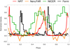 |
Fig. 1. Multi-wavelength pulse profiles of PSR J0740+6620 as observed in radio with NenuFAR (39–76 MHz, orange line) and NRT (1.4 GHz, red line), in X-rays with NICER (energy band 0.3 − 1.5 keV, green line), and in γ rays with the Fermi LAT (≥0.1 GeV, black line). |
2.2. NenuFAR profile
On 2024-03-13, we observed PSR J0740+6620 with NenuFAR (New extension in Nançay upgrading LOFAR, see Zarka et al. 2015), (Zarka et al. in prep.), using the LUPPI backend (Bondonneau et al. 2021). We recorded data from 39 to 76 MHz. We refolded the NenuFAR observations using the Nançay Radio Telescope (NRT) timing solution except for the DM value, for which the value determined directly from the NenuFAR observations is considerably more precise, owing to the low-frequency coverage of NenuFAR.
PSR J0740+6620 is among the twelve MSPs detected by NenuFAR, (Bondonneau et al. 2021). The NenuFAR profile of the pulsar considerably differs from that obtained by NRT. It has only one peak (rather than two). The main peak seems to be wider at NenuFAR frequencies. At NRT frequencies, the main peak is clearly asymmetric, with a gradual leading edge and a step trailing edge. At NenuFAR frequencies, the low S/N does not allow for definitive conclusions, but the mean peak seems to have a steeper leading edge and a gradual trailing edge. With the available data, we cannot rule out profile frequency evolution, making the comparison between the phases of the main peaks of NRT and NenuFAR difficult. Within error margins, our observations are compatible with the radio emission detected by NenuFAR and NRT being emitted at the same rotational phase. Also, the low S/N of the NenuFAR observation does not allow for an analysis of polarisation properties at those frequencies.
2.3. NICER pulse profile
To produce the X-ray pulse profile from NICER data, we processed all data from 2018-09-21 to 2024-08-31 (ObsID 1031020101 to 7031020525) using the task nicerl2 (from NICERDAS v13.0 distributed with HEASOFT v6.34) and its default filtering criteria. The most recent calibration file (v20240206) was used for this step. Then, the package NICERsoft2 was used to include additional filtering conditions. Specifically, we excluded observing periods with the following: 1) Earth magnetic cut-off rigidity COR_SAX < 1.5 GeV/c, 2) space weather index KP ≥5, 3) overshoot rates larger than 1.5 c/s, and 4) median undershoot rates larger than 100 c/s. Finally, a count-rate cut was performed to exclude all time intervals where the rate was larger than 1 c/s in the 2 − 10 keV range, where the pulsar thermal emission is negligible, which effectively removed all remaining periods of high background. The pulse phase of each individual photon was then calculated with the task photonphase (of the package PINT version v1.03) using the timing solution from the 3 PC catalogue of Fermi LAT pulsars (Smith et al. 2023). Finally, the event files of each ObsID were merged into a single event file to make the pulse profile of this pulsar with 32 phase bins (see Fig. 1). The pulse profile was produced with 32 bins in the energy range 0.3 − 1.5 keV, that is, the energy range where the thermal emission is significant (Riley et al. 2021; Miller et al. 2021).
3. Magnetic field determination
The geometry of the dipole magnetic field of several MSPs has already been investigated with a simple striped wind model relying on the split monopole (Pétri 2011). More recently, Benli et al. (2021) used the numerical solution of the pulsar force-free magnetosphere to deduce the large-scale dipole geometry for another sample of MSPs. The simplest deviation from a dipolar magnetosphere assumes an off-centred dipole, displaced with respect to the centre of the star. This configuration has been extensively studied analytically by Pétri (2021) and Pétri (2019), including polarisation (Pétri 2017). However, as a simple first guess outside the light cylinder, a centred dipole offers a minimalistic model with the fewest parameters to be fitted. We started with this assumption.
3.1. Dipole geometry from γ-ray modelling
The γ-ray light-curve fitting procedure has been explained in depth in Benli et al. (2021) and Pétri & Mitra (2021). In summary, the two main parameters to be adjusted are the γ-ray light-curve peak separation, Δ, and the phase lag, δ, between the first γ-ray peak and the radio profile. The third Fermi LAT pulsar catalogue reports a peak separation of Δ = 0.462 and a radio time lag of δ = 0.196. To a very good approximation, Pétri (2011) showed that the peak separation, Δ, is related to the pulsar obliquity, α, and line-of-sight inclination angle, ζ, by
 (1)
(1)
However, as in radio, the γ-ray profile may be asymmetric such that the phase location of the peak intensity does not necessarily correspond to the middle of the pulse profile, and thus the measurement of Δ could be altered if another definition is used for the separation, Δ. In the particular case of PSR J0740+6620, we checked that the peak separation approach gives the same results as for the separation obtained from measuring the width at 30% peak intensity except for a slight shift in phase (see Table 1). However, the width at 20% peak intensity leads to a smaller peak separation of Δ = 0.44. Moreover, as the radio pulse profile shows a pulse and an interpulse, this pulsar should be close to an orthogonal rotator. Nevertheless, we emphasise that a pulse with an interpulse could also be explained by an almost-aligned rotator, as demonstrated by Hankins & Cordes (1981). Because γ-rays are detected simultaneously with radio photons, however, such geometry is forbidden, and the constraints on the line of sight, ζ, and obliquity, α, are more stringent (see the green shaded area in Fig. 2 and Figure 2 of Pétri (2024) for the condition to simultaneously detect radio and γ-rays). Moreover NICER pulse profile modelling gives a line-of-sight inclination angle of ζ ≈ 87°, assuming roughly spin-orbit alignment, which is also incompatible with an almost-aligned rotator that we thus discarded.
Phase locations of the first and second pulse profile peaks in radio, X-ray, and γ-ray.
Therefore, the presence of a pulse and an interpulse puts stringent constraints on the geometry because the radio pulses emanating from both poles can only be detected if |ζ − π/2|< ρ and |α − π/2|< ρ are simultaneously satisfied, where ρ is the radio beam cone opening angle. This condition is given by the green shaded area in Fig. 2, where we assume a radio beam cone half-opening angle of ρ = 38°, which is the minimal opening angle required for detecting the main radio pulse and the interpulse if the γ peak separation is Δ ≈ 0.46. We concluded that the beam size must be at least as large as 38° because the peak separation would otherwise always be larger than Δ ≳ 0.46. The minimal cone opening angle is given by the geometry imposing ζ = α. For this particular configuration, by setting α ≈ ζ, we obtained  . This led to a first guess of the geometry given by α ≈ ζ ≈ 71°. In order to get Δ ≲ 0.462, however, we needed to impose a radio cone beam with a half-opening angle of ρ ≳ 38° if either α or ζ is changed. Indeed, the NICER collaboration reports ζ ≈ 87°, implying larger radio cone beams. Taking ζ ≈ 87° leads to an obliquity of α ≈ 24° and a cone opening angle of ρ ≈ 69°. However, this geometry is incompatible with the detection of a main pulse and an interpulse. In any case, requiring a higher inclination of the line of sight would lead to lower obliquities. For instance, if ζ ≈ 80°, we would require α ≈ 56°, and obtaining two radio pulses becomes less and less probable.
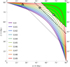 |
Fig. 2. Constraints on the viewing angle and obliquity. For symmetry reasons, the other three quadrants are not shown. Colours indicate the value of the peak separation, Δ, from 0.41 in violet to 0.49 in red. The white circle, square, and triangle show the location of three possible fits to the γ-ray peak separation with (α, ζ) respectively as (71° ,71° ), (51° ,82° ), and (24° ,87° ). The green area highlights the region in the diagram where γ-ray emission is detected simultaneously with the radio pulse for (α, ζ) = (71° ,71° ). The other dashed and dotted line delimit the same region but for (α, ζ) = (51° ,82° ) and (α, ζ) = (24° ,87° ), respectively. |
To obtain independent constraints on these angles, we performed a fit of the γ-ray light curve as shown in Fig. 3 using the same model as Benli et al. (2021). A good fit to this γ-ray light-curve with two radio pulses is given by α = 51° and ζ = 82°, as shown in Fig. 4. To accurately fit the γ-ray peak time lag with respect to the radio peak, we added a third parameter, which is depicted by the phase shift and denoted by ϕ, as done in our previous works. Its value, however, remains small, ϕ = 0.02. The associated radio beam opening angle is ρ ≈ 50°, which is compatible with the detection of two radio pulses.
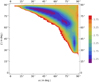 |
Fig. 3. Best-fit angles of α and ζ for the PSR J0740+6620 γ-ray light curve. The lowest values of χ2, whose colour-coding is in the legend, represents the preferred values. |
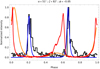 |
Fig. 4. Example of a good fit of the γ-ray pulse profile (≥0.1 GeV). The radio pulse profile is shown in red, our model for the radio component is displayed in orange, the γ-ray profile is shown in black, and the fit of the γ-ray component is shown in blue. |
On the one hand, radio and γ-rays furnish some constraints on the geometry. On the other hand, X-ray pulse profile modelling is now able to deduce the polar cap shapes, locations, and temperatures detected as atmospheric emission from hot spots. Actually, these hot spots are heated by the bombardment of charged particles produced in the magnetosphere and partly returning to the stellar surface. These particles are also responsible for the radio emission. There is therefore a one-to-one correspondence between polar caps and hot spots. These measurements by the NICER collaboration provide independent constraints on the dipole or multipole magnetic field geometry, which we exploit in the following. However, we stress that there is a degeneracy in the geometry found for the two hot spots because they can be flipped.
3.2. Dipole geometry from X-ray pulsations
For the MSP PSR J0740+6620, Riley et al. (2021) report a radius of R = 12.39 km and a mass of M = 2.07 M⊙ and thus a ratio of stellar radius to light-cylinder radius a = R/rL ≈ 0.091, with rL = c/Ω. Based on the pulse profile evolution with energy, they also deduced the polar cap geometry, assuming only a pair of circular hot spots. Moreover, the relatively low signal-to-noise ratio of the data do not allow more complex hot spot shapes to be tested. Independent constraints from a second group (Miller et al. 2021) were also reported. We used the latest results of Salmi et al. (2024b) and Dittmann et al. (2024) as best-fit parameters, summarised in Table 2 as the median of the posterior distributions (‘median’) and the value at maximum likelihood (ML), which may differ from the median for non-symmetric distributions. The parameters (Θp, Θs) on one side and (ϕp, ϕs) on the other side define the centre of the primary, p, and secondary, s, hot spot colatitude and initial phase, whereas ζp and ζs are their angular sizes. The geometry of the off-centred dipole with the parameters (α, β, δ, ϵ) defined in Pétri (2017) were then deduced and are shown in the right columns in the same table. We found a mildly off-centred dipole structure with a displacement, d, such that ϵ = d/R ≈ 0.22.
Off-centred dipole geometry deduced from the polar cap location after the new joint NICER and XMM-Newton results of [1] (Salmi et al. 2024b) and from [2] (Dittmann et al. 2024).
The magnetic obliquity is α ≈ 72° in the median case and α ≈ 78° in the ML case for the Salmi et al. (2024b) results. A similar geometry for the ML case has been reported by Dittmann et al. (2024). This is, however, 20° more than the obliquity found by the γ-ray light-curve fitting, although the inclination angle is within 5° of the NICER results. It would be enlightening to redo the X-ray pulse profile modelling and observe the variation induced on α by removing the constraint on ζ, as it would allow for lower values, for instance, closer to ζ = 80° and to check whether these new values would be more compatible with the previous γ-ray fit.
3.3. X-ray and γ-ray time lag
Our light-curve fitting procedure relies heavily on multi-wavelength phase aligned pulse profiles. The most important characteristics of these profiles are the phase of the peaks in γ-ray and X-ray. For the radio pulse profile, the situation is less obvious. We could use the peak value or the centre of the radio pulse profile defined for instance by the interval containing at least 5% or 10% of the peak intensity. We believe that the latter is more robust and chose the phase of the centre to lie halfway between the phases of 10% peak intensity of the corresponding pulse.
Table 1 summarises the locations of the pulse centres as defined above. The X-ray pulse peaks both arrive slightly before the middle of the radio pulse profile. This ordering is incompatible with the off-centred dipole geometry because the order of appearance of radio and X-rays should be inverted between the north and south pole for simple circular polar cap shapes. This one-sided phase lag between the X-ray and radio pulses requires an accurate quantitative geometric study of the location of the peak X-ray emission within the hot spot. On top of the geometry, to estimate the time lag, a careful analysis of aberration, retardation (A/R) and magnetic sweep-back effects must be included in a detailed analysis of the different wavelengths (Phillips 1992). This, however, is out of the scope of this work (but see the discussion in Sect. 4 for orders of magnitude estimates).
The X-ray pulse peaks are separated by approximately 0.4 in phase. Looking at Table 2, we therefore associated the first X-ray pulse denoted by P1X to the primary hot spot location at Θp, thus in the northern hemisphere, whereas the second X-ray pulse, denoted by P2X, is attributed to the secondary hot spot location at Θs, thus in the southern hemisphere. At radio frequencies, the peak separation is also about 0.45 in phase, and thus the second radio pulse, denoted by P2R, is linked to P1X, whereas the first radio pulse, denoted by P1R, is linked to P2X. One X-ray pulse centre leads its radio pulse centre by a phase shift of about 0.1, while the other X-ray pulse centre is almost aligned with its radio pulse centre.
3.4. Radio emission and polarisation
Some more information can be gained from studying the radio pulse profiles and their polarisation. It is well known that the width, W, is related to the beam cone half-opening angle, ρ, by (Gil et al. 1984)
 (2)
(2)
Moreover, if we assume that the full open field line region is producing radio photons, then ρ is related to the polar cap size by  . The pulse widths at 5% maximum intensity for the first and second radio peak are respectively w5 = {0.164, 0.233}. The pulse width imposes some constraints on α and ζ, as shown in Fig. 5. To estimate the beam opening angle, we compared the three geometries, namely the minimalistic ζ = α = 71°, the best γ-ray fit (α, ζ) = (51° ,82° ), and the NICER fit (α, ζ) = (24° ,87° ). The corresponding radio beam cone half-opening angle for one pole is then, respectively, 39.5° ,49° , and 69°, and for the other, it is 48° ,56° , and 72°. For these inclination angles, we get for the P2 width w5 = 0.233 the following opening angles: 39.5° ,49° , and 69°. For the P1 width w5 = 0.164, the opening angles we obtained are 48° ,56° , and 72°. The values are summarised in Table 3. These angles can be related to emission heights, he, (Pétri 2024) with
 (3)
(3)
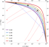 |
Fig. 5. Constraints on the geometry with fixed radio pulse profiles. The red dashed curve constrains the width at 5% maximum intensity, as given by w5 = 0.233, whereas the blue dashed curve constrains w5 = 0.164 for three values of ζ. |
Radio beam cone opening angle, ρ, according to different geometries of the pulsar giving ρ in the first part and he/rL in the second part separated by a forward slash.
and these are also reported in the same table. The emission heights correspond to a substantial fraction of the light-cylinder radius, between 20% and 50% of rL. At these altitudes, some plasma effects will distort the dipole field and the approximation used in Eq. (3) becomes inaccurate.
Moreover, the cone opening angle ρ is not compatible with the hot spot angular sizes ξp and ξs found by the NICER collaboration. Indeed if we assume that the rim of the almost circular hot spot corresponds to the edge of the radio emission beam, then the emission height, h, is given by
 (4)
(4)
with θ as the colatitude at which the radio beam has an opening angle, ρ. For a pure static dipole, both angles are related by
 (5)
(5)
For ξp, s ≲ 0.125, we always find h ≳ rL, and therefore the radio emission would be produced outside the light cylinder. One possible conclusion is that the hot spot radiating X-ray is not directly connected to the large-scale dipole field because a bombardment of particles onto the polar caps would lead to much larger circular spots of angular size, ξ ∼ 0.3. This also means that the magnetic moment vector does not necessarily intersect the hot spots, and therefore the magnetic obliquities given in Table 2 are subject to large uncertainties. Another possibility is to split the dipole into a double dipole geometry where two dipoles coexist and are located just underneath the surface of both hot spots. Figure 6 shows an example of a double dipole geometry contained in the equatorial plane with two dipoles of same magnitude. The field lines look very similar to a single dipole at large distance but close to the surface, and the non-antipodal location of the magnetic pole is visible. We explore this idea deeper in the discussion section below.
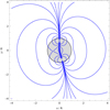 |
Fig. 6. Example of double dipole geometry in the equatorial plane. Magnetic field lines are shown in blue, and the neutron star surface is shown as a solid black circle of normalised radius. The stellar interior is shown in light gray. |
The PPA evolution can be used to help check the consistency of the magnetic geometry. In Fig. 7, we show PPA values as obtained from a high signal-to-noise ratio observation of PSR J0740+6620 conducted with the NRT at 1.4 GHz on MJD 59576 (2021-12-13). The Stokes parameters were calibrated using the method presented in Guillemot et al. (2023) and were corrected for Faraday rotation using the rotation measure value of −31 rad m−2 determined from the data themselves using the rmfit tool of PSRCHIVE (Hotan et al. 2004). Relying on the rotating vector model of Radhakrishnan & Cooke (1969), Fig. 7 shows a good fit to the data with α = 79° and ζ = 89°, fitting P1R and P2R simultaneously. We assumed that the PPA shows orthogonal mode switching for P2R depending on the phase. One mode has 0.4 < ϕ < 0.53 and the other has 0.53 < ϕ < 0.6. Because P2R is not shifted by half a period compared to P1R, we also tried a fit by translating P2R to earlier phases by an amount of Δϕ = −0.03 (brown shifted curve). This ensures the antipodal position required for the RVM fitting formula instead of fitting P1R and P2R individually. In the shifted approach, one single set of parameters is sufficient for both pulses. The associated fit is slightly better than the unshifted case, but the geometry remains almost unchanged, with α = 74° and ζ = 88° instead of α = 79° and ζ = 89° for the unshifted black curve.
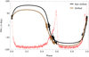 |
Fig. 7. Polarisation position angle as a function of rotational phase for PSR J0740+6620 as measured with the NRT at 1.4 GHz. The best values for the non-shifted PPA are α = 79° and ζ = 89°, whereas for the PPA shifted in phase by 0.03, the values are α = 74° and ζ = 88°. The radio pulse profile is shown in red for better identification of both pulses. |
4. Discussion
The results from our γ-ray light-curve fitting and from the NICER results are subject to some caveats. First, the Fermi LAT peak separation relies on the phase difference between the peak intensity of both pulses from which Δ is deduced. However, for PSR J0740+6620, the profile is asymmetric between the leading and trailing edge, rising sharply and decreasing much more smoothly in both peaks. This raises the question about the precise location of the centre of each peak. It is unclear whether the peak separation, Δ, should be computed according to the peak intensity, as done in Fermi 3 PC, or it should be extracted from the phase centre of each pulse defined by a width at 10% maximum intensity, for instance. If we allow for an uncertainty in the estimate of Δ from the plot in Fig. 2, we stress that at a large line-of-sight inclination angle, ζ ≳ 80°, the obliquity, α, becomes very sensitive to the value of Δ. A slight increase in Δ can lead to a drastic increase in α. For instance, when choosing Δ = 0.48 and keeping ζ = 82°, we would find α = 66° much closer to the 72° found by NICER.
Secondly, the NICER collaboration assumes that the orbital plane inclination angle, i, is equal to the observer line-of-sight inclination angle, ζ, and thus i = ζ. But this is valid only if the pulsar had enough time to exactly align its spin axis with the orbital angular momentum. Whether the accretion phase was efficient and long enough to proceed to exact alignment is unclear, and a small deviation of several degrees might be possible.
Third, the magnetic axis was assumed to cross the centre of each hot spot, implying that the heating of the polar caps by particle bombardment is circularly symmetric. However, this assumption, too, needs to be corrected, as there should be a sweepback of magnetic field lines and some other effects related to the stellar rotation. Therefore, the values for (α, β, δ, ϵ) shown in Table 2 should be reevaluated in light of these caveats.
Finally, the angular size of both hot spots are very similar, ξp ≈ ξs ≈ 0.115. However the usual size of the polar cap, deduced from the opening field line region gives a value of  ; thus, it is almost a factor of three larger for this estimate about a centred dipole. As we showed in Pétri et al. (2023), an off-centring of the dipole location can drastically reduce the size of the polar cap. If for simplicity we assume an aligned rotator and shift the dipole along the rotation axis to the south pole, the displacement, z0, required to adjust the spot size to an angle, ξp, while dropping the negative solution is given by
 (6)
(6)
By inputting numbers adapted for PSR J0740+6620, we find that a shift of z0/rL ≈ 0.077 is sufficient to reduce the polar cap size to the observed value. This corresponds to a distance z0 ≈ 10.7 − 11.1 km and thus to a size related to the neutron star radius of z0/R ≈ 0.85 − 0.89. The dipole is located slightly underneath the surface, i.e., in the crust. The same idea can be applied to the south polar cap with a similar shift.
Because the light-cylinder radius is only 11 times larger than the stellar radius with R/rL ≈ 0.091, the impact of an off-centred or a double dipole remains substantial for the geometry of the current sheet in the striped wind. Indeed the perfect symmetry in the light curves is broken for those configurations, and the relation between the angles α and ζ and the peak separation, Δ, deviates slightly from the analytical expectations given by Eq. (1). Variations in Δ of about 0.01 − 0.02 are easily achievable for MSPs. The impact on the obliquity, α, for high inclination angles, ζ, around 85° is dramatic, as shown in Fig. 2. Setting, for instance, the value for ζ approximately to 82° or 87°, we found the obliquities shown in Table 4. The peak separation is not the most reliable property of the light curves, especially if the leading and trailing edges of the pulses are asymmetric. Scrutiny of the full shape is therefore recommended because the pulse centre then shifts from the peak intensity. Nevertheless, within a few degrees of uncertainties, the radio emission and PPA fit agrees with the γ-ray light curve and with the location of the thermal hot spots. This gives us confidence about the robustness of the double dipole approach for such a recycled pulsar.
Obliquity, α, of the magnetic field for varying peak separation, Δ, and different inclination angles, ζ.
To be more quantitative, Fig. 8 shows an example of variation of the γ-ray peak separation, Δ, when an off-centred dipole is taken into account. We computed the force-free magnetosphere solutions for α = 70°, β = 0°, δ = 90° and ϵ = {0.2, 0.4} and then extracted the γ-ray light curves as presented in Fig. 8. In this particular case with ζ = 82°, the off-centring increases the peak separation, Δ, by approximately 0.02 in phase for both eccentricities (ϵ = 0.2 and ϵ = 0.4) compared to the centre dipole, as shown by the green and orange curves that almost overlap with this viewing angle. Therefore, for fast-rotating MSPs, the peak separation measurements are not sufficient to robustly estimate the geometry of the large-scale dipolar magnetic field. Some cross-checks using multi-wavelength data are required, as we demonstrated in this work.
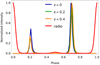 |
Fig. 8. Comparison of the simulated γ-ray light curves between the centred dipole in blue and the off-centred dipole in green and orange for α = 70°, β = 0°, δ = 90°, and ϵ = 0.2. The line-of-sight inclination is ζ = 82°. The radio pulse profile is shown in red. |
Finally, knowing the radio emission height, denoted by r2, and setting the thermal X-ray emission radius to r1 = R, we can estimate the delays introduced by aberration, Δta; retardation, Δtr; and sweepback, ΔtB, effects for which the magnitude increases with increasing altitude according to Phillips (1992) because
 (7a)
(7a)
![Mathematical equation: $$ \begin{aligned} \frac{\Delta t_{\rm a}}{P}&= \frac{\arctan \left[(r_1/ r_\text{L}) \sin \right] - \arctan \left[ ( r_2 / r_\text{L}) \sin \right]}{2\,\pi } \end{aligned} $$](/articles/aa/full_html/2025/09/aa55574-25/aa55574-25-eq11.gif) (7b)
(7b)
![Mathematical equation: $$ \begin{aligned} \frac{\Delta t_{\text{ B}}}{P}&= \frac{1.2\,\sin ^2}{2\,\pi } \, \left[\left( \frac{r_2}{r_\text{L}} \right)^3 - \left( \frac{r_1}{r_\text{L}} \right)^3 \right]. \end{aligned} $$](/articles/aa/full_html/2025/09/aa55574-25/aa55574-25-eq12.gif) (7c)
(7c)
From the previous section, we found a maximum radio emission height of about 40 − 50% of rL at which aberration and retardation effects each contribute approximately equally to 6% of the phase advance, whereas vacuum magnetic field sweepback contributes approximately 2.5% of phase retardation, leading to a total of 10% phase advance of the radio pulse compared to the thermal X-ray emission. If, however, we use the more realistic force-free magnetic field sweepback effect instead of the vacuum one, the term involving ΔtB contributes approximately six times more than in the vacuum (see for instance Figure 6 of Pétri 2024), thus adding 15% to the phase retardation. In all, the force-free sweepback compensates for the A/R phase advance, leading to almost phase-aligned radio and X-ray, as observed for PSR J0740+6620. More detailed calculations would require an exact determination of the radio emission height and the full force-free magnetosphere geometry using, for instance, the double dipole configuration shown in Figure 6. However, we do not dive into such refinements in this study.
5. Conclusions
Although MSP emission is usually thought to be difficult to model with a dipolar magnetic field because of the impact of multipolar components close to the stellar surface, we have shown that a double dipole geometry can confidently reproduce a wealth of multi-wavelength properties of PSR J0740+6620. A mildly off-centred dipole would be compatible with radio, thermal X-ray, and γ-ray pulse profiles, but the size of the heated polar cap would be three times larger than the expected size deduced from the NICER collaboration. Both dipoles are almost antipodal and located approximately 10% below the surface. Whether such a configuration could be applied to other MSPs must be tested case by case. Good candidates include those from other NICER pulsars with published results, such as PSR J0437-4715 (Choudhury et al. 2024) or PSR J1231-1411 (Salmi et al. 2024a). We plan to investigate these pulsars in the near future.
Acknowledgments
We are grateful to the referee for helpful comments and suggestions. This work has been supported by the ANR (Agence Nationale de la Recherche) grant number ANR-20-CE31-0010. SG and DGC acknowledge the support of the CNES. This paper is partially based on data obtained using the NenuFAR radio-telescope. The development of NenuFAR has been supported by personnel and funding from: Observatoire Radioastronomique de Nançay, CNRS-INSU, Observatoire de Paris-PSL, Université d’Orléans, Observatoire des Sciences de l’Univers en Région Centre, Région Centre-Val de Loire, DIM-ACAV and DIM-ACAV + of Région Ile-de-France, Agence Nationale de la Recherche. The Nançay Radio Observatory (NRT) is operated by the Paris Observatory, associated with the French Centre National de la Recherche Scientifique (CNRS) and Université d’Orléans. It is partially supported by the Région Centre Val de Loire in France. We acknowledge the use of the Nançay Data Centre computing facility (CDN – Centre de Données de Nançay). The CDN is hosted by the Observatoire Radioastronomique de Nançay (ORN) in partnership with Observatoire de Paris, Université d’Orléans, OSUC, and the CNRS. The CDN is supported by the Région Centre-Val de Loire, dpartement du Cher. The Nançay Radio Observatory (ORN) is operated by Paris Observatory, associated with the French Centre National de la Recherche Scientifique (CNRS) and Université d’Orléans.
References
- Benli, O., Pétri, J., & Mitra, D. 2021, A&A, 647, A101 [NASA ADS] [CrossRef] [EDP Sciences] [Google Scholar]
- Bondonneau, L., Grießmeier, J.-M., Theureau, G., et al. 2021, A&A, 652, A34 [NASA ADS] [CrossRef] [EDP Sciences] [Google Scholar]
- Choudhury, D., Salmi, T., Vinciguerra, S., et al. 2024, ApJ, 971, L20 [NASA ADS] [CrossRef] [Google Scholar]
- Cromartie, H. T., Fonseca, E., Ransom, S. M., et al. 2020, Nat. Astron., 4, 72 [NASA ADS] [CrossRef] [Google Scholar]
- Dittmann, A. J., Miller, M. C., Lamb, F. K., et al. 2024, ApJ, 974, 295 [NASA ADS] [CrossRef] [Google Scholar]
- Fonseca, E., Cromartie, H. T., Pennucci, T. T., et al. 2021, ApJ, 915, L12 [NASA ADS] [CrossRef] [Google Scholar]
- Gil, J., Gronkowski, P., & Rudnicki, W. 1984, A&A, 132, 312 [NASA ADS] [Google Scholar]
- Guillemot, L., Smith, D. A., Laffon, H., et al. 2016, A&A, 587, A109 [NASA ADS] [CrossRef] [EDP Sciences] [Google Scholar]
- Guillemot, L., Cognard, I., van Straten, W., Theureau, G., & Gérard, E. 2023, A&A, 678, A79 [NASA ADS] [CrossRef] [EDP Sciences] [Google Scholar]
- Hankins, T. H., & Cordes, J. M. 1981, ApJ, 249, 241 [NASA ADS] [CrossRef] [Google Scholar]
- Hotan, A. W., van Straten, W., & Manchester, R. N. 2004, PASA, 21, 302 [Google Scholar]
- Johnston, S., Kramer, M., Karastergiou, A., et al. 2023, MNRAS, 520, 4801 [Google Scholar]
- Miller, M. C., Lamb, F. K., Dittmann, A. J., et al. 2019, ApJ, 887, L24 [Google Scholar]
- Miller, M. C., Lamb, F. K., Dittmann, A. J., et al. 2021, ApJ, 918, L28 [NASA ADS] [CrossRef] [Google Scholar]
- Pétri, J. 2011, MNRAS, 412, 1870 [Google Scholar]
- Pétri, J. 2017, MNRAS, 466, L73 [CrossRef] [Google Scholar]
- Pétri, J. 2019, MNRAS, 488, 4161 [Google Scholar]
- Pétri, J. 2021, MNRAS, 501, 4479 [Google Scholar]
- Pétri, J. 2024, A&A, 687, A169 [NASA ADS] [CrossRef] [EDP Sciences] [Google Scholar]
- Pétri, J., & Mitra, D. 2021, A&A, 654, A106 [NASA ADS] [CrossRef] [EDP Sciences] [Google Scholar]
- Pétri, J., Guillot, S., Guillemot, L., et al. 2023, A&A, 680, A93 [NASA ADS] [CrossRef] [EDP Sciences] [Google Scholar]
- Pétri, J., Guillot, S., Guillemot, L., et al. 2024, A&A, 687, L13 [NASA ADS] [CrossRef] [EDP Sciences] [Google Scholar]
- Phillips, J. A. 1992, ApJ, 385, 282 [NASA ADS] [CrossRef] [Google Scholar]
- Radhakrishnan, V., & Cooke, D. J. 1969, Astrophys. Lett., 3, 225 [NASA ADS] [Google Scholar]
- Riley, T. E., Watts, A. L., Bogdanov, S., et al. 2019, ApJ, 887, L21 [Google Scholar]
- Riley, T. E., Watts, A. L., Ray, P. S., et al. 2021, ApJ, 918, L27 [CrossRef] [Google Scholar]
- Salmi, T., Vinciguerra, S., Choudhury, D., et al. 2022, ApJ, 941, 150 [CrossRef] [Google Scholar]
- Salmi, T., Deneva, J. S., Ray, P. S., et al. 2024a, ApJ, 976, 58 [Google Scholar]
- Salmi, T., Choudhury, D., Kini, Y., et al. 2024b, ApJ, 974, 294 [NASA ADS] [CrossRef] [Google Scholar]
- Smith, D. A., Abdollahi, S., Ajello, M., et al. 2023, ApJ, 958, 191 [NASA ADS] [CrossRef] [Google Scholar]
- Vinciguerra, S., Salmi, T., Watts, A. L., et al. 2024, ApJ, 961, 62 [NASA ADS] [CrossRef] [Google Scholar]
- Wahl, H. M., McLaughlin, M. A., Gentile, P. A., et al. 2022, ApJ, 926, 168 [NASA ADS] [CrossRef] [Google Scholar]
- Wolff, M. T., Guillot, S., Bogdanov, S., et al. 2021, ApJ, 918, L26 [Google Scholar]
- Zarka, P., Tagger, M., Denis, L., et al. 2015, 2015 International Conference on Antenna Theory and Techniques (ICATT), 1 [Google Scholar]
All Tables
Phase locations of the first and second pulse profile peaks in radio, X-ray, and γ-ray.
Off-centred dipole geometry deduced from the polar cap location after the new joint NICER and XMM-Newton results of [1] (Salmi et al. 2024b) and from [2] (Dittmann et al. 2024).
Radio beam cone opening angle, ρ, according to different geometries of the pulsar giving ρ in the first part and he/rL in the second part separated by a forward slash.
Obliquity, α, of the magnetic field for varying peak separation, Δ, and different inclination angles, ζ.
All Figures
|
Fig. 1. Multi-wavelength pulse profiles of PSR J0740+6620 as observed in radio with NenuFAR (39–76 MHz, orange line) and NRT (1.4 GHz, red line), in X-rays with NICER (energy band 0.3 − 1.5 keV, green line), and in γ rays with the Fermi LAT (≥0.1 GeV, black line). |
| In the text | |
|
Fig. 2. Constraints on the viewing angle and obliquity. For symmetry reasons, the other three quadrants are not shown. Colours indicate the value of the peak separation, Δ, from 0.41 in violet to 0.49 in red. The white circle, square, and triangle show the location of three possible fits to the γ-ray peak separation with (α, ζ) respectively as (71° ,71° ), (51° ,82° ), and (24° ,87° ). The green area highlights the region in the diagram where γ-ray emission is detected simultaneously with the radio pulse for (α, ζ) = (71° ,71° ). The other dashed and dotted line delimit the same region but for (α, ζ) = (51° ,82° ) and (α, ζ) = (24° ,87° ), respectively. |
| In the text | |
|
Fig. 3. Best-fit angles of α and ζ for the PSR J0740+6620 γ-ray light curve. The lowest values of χ2, whose colour-coding is in the legend, represents the preferred values. |
| In the text | |
|
Fig. 4. Example of a good fit of the γ-ray pulse profile (≥0.1 GeV). The radio pulse profile is shown in red, our model for the radio component is displayed in orange, the γ-ray profile is shown in black, and the fit of the γ-ray component is shown in blue. |
| In the text | |
|
Fig. 5. Constraints on the geometry with fixed radio pulse profiles. The red dashed curve constrains the width at 5% maximum intensity, as given by w5 = 0.233, whereas the blue dashed curve constrains w5 = 0.164 for three values of ζ. |
| In the text | |
|
Fig. 6. Example of double dipole geometry in the equatorial plane. Magnetic field lines are shown in blue, and the neutron star surface is shown as a solid black circle of normalised radius. The stellar interior is shown in light gray. |
| In the text | |
|
Fig. 7. Polarisation position angle as a function of rotational phase for PSR J0740+6620 as measured with the NRT at 1.4 GHz. The best values for the non-shifted PPA are α = 79° and ζ = 89°, whereas for the PPA shifted in phase by 0.03, the values are α = 74° and ζ = 88°. The radio pulse profile is shown in red for better identification of both pulses. |
| In the text | |
|
Fig. 8. Comparison of the simulated γ-ray light curves between the centred dipole in blue and the off-centred dipole in green and orange for α = 70°, β = 0°, δ = 90°, and ϵ = 0.2. The line-of-sight inclination is ζ = 82°. The radio pulse profile is shown in red. |
| In the text | |
Current usage metrics show cumulative count of Article Views (full-text article views including HTML views, PDF and ePub downloads, according to the available data) and Abstracts Views on Vision4Press platform.
Data correspond to usage on the plateform after 2015. The current usage metrics is available 48-96 hours after online publication and is updated daily on week days.
Initial download of the metrics may take a while.