| Issue |
A&A
Volume 701, September 2025
|
|
|---|---|---|
| Article Number | A80 | |
| Number of page(s) | 11 | |
| Section | Numerical methods and codes | |
| DOI | https://doi.org/10.1051/0004-6361/202555911 | |
| Published online | 05 September 2025 | |
An inversion approach to retrieve the vector magnetic field from scattering polarization in strong solar resonance lines
1
Istituto ricerche solari Aldo e Cele Daccò (IRSOL), Faculty of Informatics, Università della Svizzera italiana (USI),
6605
Locarno,
Switzerland
2
Euler Institute, Università della Svizzera italiana (USI),
6900
Lugano,
Switzerland
3
Institute for Solar Physics (KIS),
Georges-Khöler-Allee 401a,
79110
Freiburg,
Germany
4
Faculty of Mathematics, University of Belgrade,
Studentski Trg 16,
11000
Belgrade,
Serbia
5
Astronomical Observatory,
Volgina 7,
11060
Belgrade,
Serbia
★ Corresponding author: This email address is being protected from spambots. You need JavaScript enabled to view it.
Received:
12
June
2025
Accepted:
11
July
2025
Abstract
Context. Inferring the weak magnetic field present in the outer layers of the solar atmosphere is a long-standing challenge in modern solar physics. Spectropolarimetric diagnostic techniques based on the Zeeman effect are ineffective in this context, highlighting the need for alternative approaches.
Aims. Our goal is to develop a novel inference method that fits a depth-dependent vector magnetic field in a solar model atmosphere to observations of Hanle and Zeeman signals from strong resonance lines, including partial frequency redistribution (PRD) effects.
Methods. We assumed that the thermal stratification of the atmosphere is given, and we used an efficient radiative transfer forward engine tailored to strong resonance lines, while accounting for PRD, scattering polarization, and the Hanle and Zeeman effects. By formulating the inverse problem as a nonlinear least-squares problem, we applied an efficient iterative optimization algorithm that enables an efficient retrieval of the searched magnetic field vector through fast computation of the Jacobian.
Results. We tested this inversion approach by inverting synthetic Stokes profiles of the Ca I line at 4227 Å. We successfully retrieved the original height-dependent vector magnetic and bulk velocity fields in different 1D plane-parallel models. We considered both semi-empirical models and models extracted from a snapshot of a 3D MHD simulation of the solar atmosphere.
Conclusions. Our proposed inversion tool has demonstrated its reliability and promise for inverting vector magnetic fields in strong solar resonance lines that exhibit scattering polarization. Future plans include testing the approach in more complex scenarios, featuring intricate magnetic field structures. This assessment paves the way for applying our inversion tool to new spectropolarimetric observations.
Key words: polarization / radiative transfer / scattering / methods: numerical / Sun: chromosphere / Sun: magnetic fields
© The Authors 2025
 Open Access article, published by EDP Sciences, under the terms of the Creative Commons Attribution License (https://creativecommons.org/licenses/by/4.0), which permits unrestricted use, distribution, and reproduction in any medium, provided the original work is properly cited.
This article is published in open access under the Subscribe to Open model. This email address is being protected from spambots. You need JavaScript enabled to view it. to support open access publication.
1 Introduction
During the past decades, the combination of novel observations and theoretical investigations has firmly established the fundamental role played by the magnetic field in the external layers of the solar atmosphere (e.g., Carlsson et al. 2019; De Pontieu et al. 2021). Accurately inferring the magnitude and orientation of this magnetic field is an open issue in today’s solar physics research (e.g., Heliophysics Science and Technology Roadmap for 2014–2033), and this has motivated the development of new observational facilities, such as the ViSP instrument at the Daniel K. Inouye Solar Telescope (DKIST, Rimmele et al. 2020; Rast et al. 2021), the series of CLASP sounding rocket experiments (Kano et al. 2017; Rachmeler et al. 2022), and the proposal of future mission concepts such as the Chromospheric Magnetism Explorer (CMEx)1. The inference of the vector magnetic field in the chromosphere and chromosphere-corona transition region is notoriously difficult because conventional magnetic field diagnostics, based on the Zeeman effect, lose sensitivity in such layers, and only a handful of spectral lines can probe these regions. Recent works have proposed making use of the magnetic sensitivity of the scattering polarization signals of strong resonance lines through the combined action of the Hanle, Zeeman, and magneto-optical effects (e.g., Trujillo Bueno & del Pino Alemán 2022).
The process of fitting an atmospheric model, including the magnetic field, to an observed polarization signal is known as an inversion problem. To successfully tackle an inversion problem, it is crucial to have a deep understanding of the physics underlying the formation of the observed polarization signals in the spectral lines of interest. Unfortunately, modeling the scattering polarization signals of strong resonance lines requires considerable theoretical and numerical efforts. Indeed, it is crucial to account for non-local thermodynamic equilibrium (non-LTE) effects, as well as for partial frequency redistribution (PRD; Rees & Saliba 1982; Faurobert-Scholl 1992). A major difficulty when dealing with scattering polarization signals is that their amplitude primarily depends on the anisotropy of the radiation field that, in general, depends on the detailed 3D structure of the solar atmosphere. Such anisotropy must also be estimated from the observations.
The development of non-LTE inversion techniques for interpreting spectropolarimetric observations of spectral lines formed in the upper layers of the solar atmosphere is a relatively recent effort. The majority of these inversion techniques focus on chromospheric or transition region lines polarized through the Zeeman effect (see the review by de la Cruz Rodríguez & van Noort 2017). Currently, HanleRT-TIC (Li et al. 2022, 2023, 2024) is the only code capable of inverting spectropolarimetric observations of strong resonance lines, including PRD effects and scattering polarization. The main limitation of HanleRT-TIC is its computational cost, which hinders its systematic use. Moreover, being the only active code in the field, validation of its results through comparison with another code is lacking. We also note that significant progress has recently been made in 3D spectropolarimetric inversions (see Šteˇpán et al. 2022). However, routine application to optically thick lines modeled with PRD in 3D remains beyond current capabilities.
The development of an inversion method involves a multitude of technical details (see del Toro Iniesta & Ruiz Cobo 2016; de la Cruz Rodríguez & van Noort 2017, for a deep insight in the topic). However, the three essential components of an inversion code can be identified as follows:
- (i)
A comprehensive physical model governing the generation of observables, which is crucial for identifying suitable approximations and ensuring the accuracy of the inversion process;
- (ii)
An efficient forward engine that, starting from a given atmospheric model, generates the synthetic emergent spectrum and possibly calculates its response to perturbations in the input model parameters;
- (iii)
A robust inversion engine that infers the atmospheric parameters by comparing the synthetic and observed emergent spectra, ensuring a robust convergence to the optimal solution, while also involving an accurate estimate of instrumental effects and observational uncertainties.
In this paper, we propose and test an inversion approach tailored to strong resonance lines, accounting for PRD, scattering polarization, and the Hanle and Zeeman effects, while considering 1D plane-parallel atmospheric models. As a forward engine, we rely on the TRAP4 code (Riva et al. 2025). Assuming that the thermal stratification of the atmosphere is given and it is consistent with the observed intensity spectrum (i.e., Stokes I), the inversion process focuses on jointly fitting the height-dependent bulk velocity and magnetic field vectors to the observed intensity and polarization profiles.
In Sect. 2, we lay out the main equations inherent to the (forward) non-LTE radiative transfer (RT) problem for polarized radiation, including scattering polarization and PRD effects. In Sects. 3 and 4, we present the solution strategies used in the forward and inversion engines, respectively. In Sect. 5, we report numerical experiments for the assessment of our inversion approach, providing specific inversion results in Sect. 6. We provide remarks and conclusions in Sect. 7.
2 Formulation of the problem
In this section, we first recap the non-LTE RT problem for polarized radiation, highlighting the physical processes that we include in our modeling. We then summarize the solution strategy adopted for the inversion process, presenting the considered 1D plane-parallel atmospheric model.
2.1 Non-LTE RT problem for polarized radiation
The intensity and polarization of a beam of radiation are fully described by the four-component Stokes vector

with the intensity, I, being positive and the polarization being encoded in Q, U, and V, with I2 ≥ Q2 + U2 + V2. Its propagation through a given medium, such as the plasma of a stellar atmosphere, is expressed by the RT equation for polarized radiation. Under stationary conditions, which are assumed throughout this work, the propagation in a given medium of a radiation beam of frequency ν ∈ ℝ+ and direction Ω at the spatial point r ∈ D with D⊂ℝ3, is described by the following RT equation:
 (1)
(1)
where  denotes the directional derivative along Ω, K ∈ ℝ4×4 is the propagation matrix, and ε ∈ ℝ4 is the emission vector (e.g., Landi Degl’Innocenti & Landolfi 2004). Both K and ε depend on the state of the atomic system giving rise to the considered spectral lines, which in turn depends on the radiation field I through the statistical equilibrium (SE) equations. The non-LTE RT problem thus consists of finding a self-consistent solution of Eq. (1) for the radiation field I and of the SE equations for the atomic system. This problem is, in general, integro-differential, nonlocal, and nonlinear.
In this work, we consider a two-level atom with an unpolarized lower level. Neglecting stimulated emission, the SE equations for this atomic model have an analytic solution, and it is possible to directly relate the emission vector to the incident radiation field through the redistribution matrix formalism
 (2)
(2)
where kL is the frequency-integrated absorption coefficient; R is the redistribution matrix, which accounts for PRD effects; and εth describes the contribution from atoms that are collisionally excited (thermal term). The integral appearing in the first term in the r.h.s. is generally referred to as the scattering integral. We use the expressions of R and K as derived in Bommier (1997a,b) and Landi Degl’Innocenti & Landolfi (2004), respectively. The contributions of continuum processes are easily included in the expressions of K and ε (e.g., Benedusi et al. 2022). In particular, the continuum emissivity is expressed as the sum of a scattering and a thermal term, as in Eq. (2).
2.2 Inversion solution strategy
This work assumes a 1D plane-parallel atmosphere, with depth-stratified thermodynamic and magnetic properties. The inversion approach is divided into two steps. In the first one, we retrieve the depth stratification of temperature, microturbulent velocities, and particle densities. For spatially averaged observations, these quantities can be provided by a semi-empirical atmospheric model (e.g., Milic´ & Faurobert 2012), while for spatially resolved observations, they can be fitted to the intensity spectrum (i.e., Stokes I) by applying a stand-alone inversion code, such as SNAPI (Milic´ & van Noort 2018) or STiC (de la Cruz Rodríguez et al. 2019). Notably, the application of these codes to the intensity spectrum would also provide a first estimate of the line-of-sight bulk velocity field. In this first step, we also calculate the lower-level population, as well as the continuum total opacity, scattering opacity, and thermal emissivity.
In the second step, by leveraging the highly efficient TRAP4 forward engine (Riva et al. 2025), we fit the height-dependent bulk velocity and magnetic field vectors to the observed intensity, I, and fractional polarization Q/I, U/I, and V/I profiles. We note that the magnetic field primarily influences the polarization profiles, whereas bulk velocities affect both the intensity through their line-of-sight component, and the scattering polarization via their spatial gradients. As explained by Li et al. (2022), this separation between the Stokes I inversion and the polarization profiles inversion is feasible because, in solar applications, both the magnetic splitting and the polarization degree are small enough (relative to the Doppler width and the mean intensity, respectively) to have a negligible impact on the intensity spectrum.
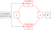 |
Fig. 1 Schematic representation of the forward non-LTE RT problem, that is, the iterative solution to determine the emergent Stokes profiles, Iout, when provided a set of atmospheric parameters, q. |
3 Forward engine
Provided a suitable discretization of the spatial, angular, and spectral coordinates (see Sect. 3.1), the calculation of the synthetic emergent Stokes profiles Iout at a specific line-of-sight, given a set of atmospheric parameters q, is known as the forward (or direct) modeling problem. This process can be represented mathematically as
 (3)
(3)
where F is the nonlinear (w.r.t. the input q) forward map, whose application can be summarized as: (i) given a set of atmospheric parameters q, one numerically solves Eqs. (1) and (2), obtaining a self-consistent (discrete) radiation field I across the entire spatial domain, encompassing all frequencies and directions; (ii) from I one can calculate the synthetic emergent Stokes profiles Iout, which are then compared with the observed profiles Iobs. This process is schematized in Fig. 1. With an abuse of notation, the vectors Iout and Iobs may also refer to fractional Stokes profiles.
This section outlines the solution strategy employed in the forward engine used in the second step of the inversion strategy, having already fixed the thermal stratification of the atmosphere. A key assumption of the adopted strategy is to consider the population of the lower level as a fixed input parameter provided by the first step. This makes the non-LTE RT problem linear w.r.t. the radiation field (e.g., Janett et al. 2021). For a detailed description and assessment of the forward engine, we refer to Benedusi et al. (2022), Janett et al. (2024), and Riva et al. (2025).
3.1 Discretization
To solve the linear forward problem, we employ a discretization of the spatial, angular, and spectral coordinates. The assumed 1D plane-parallel atmospheric model provides the spatial discretization, sampling the 1D spatial domain with Nz unevenly spaced points. The angular discretization involves sampling the unit sphere with NΩ angular points, using a tensor product of a trapezoidal quadrature for the azimuthal interval [0, 2π) and two Gauss-Legendre quadratures, one in each subinterval [−1, 0] and [0, 1], for the cosine of the inclination (corresponding to the heliocentric angle) µ. Furthermore, we discretize the finite spectral interval [νmin, νmax] ⊂ R+ with Nν unevenly spaced points, which are approximately uniformly spaced in the line core and logarithmically distributed in the line wings.
According to this discretization, we thus have  and I ∈ ℝN, with Nq = NpNz, where Np is the number of input atmospheric physical quantities and N = 4NzNΩNν represents the total number of degrees of freedom of the forward problem. We also have Iout ∈ ℝNobs and Iobs ∈ ℝNobs, where Nobs corresponds to the number of observed data, which account for all the considered Stokes components at all observed frequencies.
3.2 Algebraic formulation
The numerical solution of the RT Eq. (1) can be expressed in the compact form
 (4)
(4)
where the transfer operator Λ encodes the formal solution, ε ∈ ℝN represents the discrete emission vector, and the vector t ∈ RN represents the radiation transmitted from the boundaries. Moreover, we can express the calculation of the emission vector given by Eq. (2) as
 (5)
(5)
where the scattering operator Σ and the vector εth encode the scattering and thermal contributions to emissivity, respectively. Equations (4) and (5) are combined into the linear system
 (6)
(6)
where Id is the identity matrix. One can solve Eq. (6) to obtain the discrete radiation field I in the whole spatial domain at all frequencies and directions.
3.3 Matrix-free iterative solver
The considered forward RT problem has been recast in the linear system given by Eq. (6), for which we have to find a solution to obtain the radiation field I in the whole spatial domain at all frequencies and directions. Given the size of the system (N ≈ 107 for a typical 1D application) and that the matrix Id - ΛΣ in Eq. (6) is dense, the use of direct matrix inversion solvers is unfeasible. Thus, the application of an iterative method is preferred. The forward engine implements the generalized minimal residual (GMRES) iterative method in its matrix-free version. We monitored the convergence of the iterative method through the relative residual taking as stopping criterion res < tol, for a given tolerance tol.
3.4 Preconditioning
To increase robustness and convergence speed of iterative techniques, the forward engine employs the innovative approach to designing efficient physics-based preconditioners and initial guesses, extensively described in Janett et al. (2024). Very concisely, as P ∈ ℝN×N is a non-singular matrix, the left preconditioning of Eq. (6) is obtained by considering the equivalent system

To be effective, P should be a good and computationally cheap approximation of the operator Id - ΛΣ. When dealing with the RT non-LTE forward problem that includes scattering polarization and PRD effects, algebraic preconditioners such as Jacobi and successive over-relaxation (SOR) preconditioners are outperformed by tailored physics-based preconditioners of the form

where Λ* and Σ* encode the approximations of Λ and Σ. In the forward engine, we implemented two options for Σ*, with scattering processes modeled either with the angle-averaged approximation (e.g., Rees & Saliba 1982) or in the limit of complete frequency redistribution (CRD; e.g., Landi Degl’Innocenti & Landolfi 2004). Moreover, both Λ* and Σ* can possibly neglect polarization, the anisotropy of the emission vector in the comoving frame, and the impact of magnetic fields (Benedusi et al. 2022; Janett et al. 2024). We note that the application of P−1 requires solving a linear system of the form Px = y iteratively. To further enhance the performance of the forward engine, we also implemented the possibility of preconditioning the linear system Px = y (Riva et al. 2025).
4 Inversion engine
The process of finding the atmospheric parameters  (a.k.a. model parameters or optimization parameters) that reproduce an observed Stokes spectrum Iobs is known as the inverse problem. This process can be represented mathematically as
![Mathematical equation: \[\mathbf{I}^{\rm obs} \;\longmapsto\; F^{-1}(\mathbf{I}^{\rm obs}) = \mathbf{q}^{\rm out},\]](/articles/aa/full_html/2025/09/aa55911-25/aa55911-25-eq13.png)
where F−1 is the nonlinear (w.r.t. the input Iobs) inverse map. We note that our inverse problem is usually ill-posed, and the existence of F−1 is in general not guaranteed. In essence, the goal of an inversion is to find the atmospheric parameters qout that satisfy the condition
![Mathematical equation: \[F(\mathbf{q}^{\rm out}) = \mathbf{I}^{\rm out} \approx \mathbf{I}^{\rm obs},\]](/articles/aa/full_html/2025/09/aa55911-25/aa55911-25-eq14.png)
and this process is often addressed iteratively, as schematized in Fig. 2. Bearing in mind that the inversion process involves a significant amount of technical details, in this section, we outline the overall structure and the key aspects of the solution strategy employed in our inversion engine.
4.1 Node-based atmospheric parametrization
In forward RT calculations, the knowledge of the heightdependent Np input atmospheric physical quantities is required on a relatively dense spatial grid of size Nz. In the inverse problem, it is often impractical to directly fit the Np input atmospheric physical quantities at all Nz spatial points, as this would result in an excessively large number of unknowns, Nq = NpNz, leading to an ill-posed inversion problem (e.g., Šteˇpán et al. 2022).
To circumvent this issue (and also reduce the cost of the inversion process), it is advantageous to decouple the optimization domain from the forward problem domain. For instance, it is common to parameterize the spatial distribution of the input atmospheric physical quantities. In particular, Ruiz Cobo & del Toro Iniesta (1992) introduced the node-based inversion technique to reduce the number of unknowns in the inversion process. This approach introduces, for each height-dependent atmospheric physical quantity, a coarser spatial grid with Nm points (a.k.a. nodes), where m = 1,...,Np. Implicitly, one has Nm = 1 for height-independent atmospheric physical quantities. We collected these parameters in the vector  , where
![Mathematical equation: \[N_x = \sum_{m=1}^{N_p}N_m\]](/articles/aa/full_html/2025/09/aa55911-25/aa55911-25-eq16.png)
is the actual number of unknowns of the inversion problem; ideally, Nx ≪ Nq. The atmospheric parameters on the forward problem spatial grid are reconstructed through interpolation:
 (7)
(7)
The complexity of the fitted atmospheric model is thus determined by the number of nodes and the choice of the interpolant f. Several types of interpolations have been proposed to relate the nodes to the finer grid (e.g., de la Cruz Rodríguez et al. 2019). In our inversion approach, we provide the option to use the following interpolants: constant, linear, and shape-preserving piecewise cubic. It is essential to note that if the number of nodes Nm is excessively large, the inversion solution may exhibit oscillatory behavior or even fail to converge. Therefore, it is crucial to find a setup that can reproduce the observed spectra with the lowest number of unknowns Nx (de la Cruz Rodríguez & van Noort 2017).
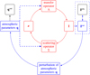 |
Fig. 2 Schematic representation of the inversion problem, that is the iterative solution to determine the atmospheric parameters, qout, that best reproduce an observed Stokes spectrum, Iobs. |
4.2 Nonlinear least squares problem
The inversion problem is usually expressed as a parameter estimation based on the minimization of a metric in the space of the observables (del Toro Iniesta & Ruiz Cobo 2016). In mathematical optimization, this metric is referred to as loss function or objective function. To compare the observed Iobs and computed Iout quantities, we used as a loss function the sum of squared residuals
 (8)
(8)
where  , with the index i encompassing all the considered Stokes components and all the available frequen-cies.2 The process of fitting an atmospheric model to an observed signal thus consists in finding the vector x that minimizes the sum of squared residuals given by Eq. (8), thereby solving the nonlinear3 least-squares problem
 (9)
(9)
4.3 Optimization iterative solver
The nonlinear least-squares problem given by Eq. (9) is typically solved using iterative processes, which are known as nonlinear least squares algorithms. The iterative approach starts with an initial guess x0 and generates a sequence of improving approximate solutions x1, x2,..., xk, xk + 1, reaching a solution xout that satisfies some predefined convergence criteria. This iterative process can be expressed in its correction form as xk+1 = xk + ∆xk, where ∆xk represents the correction. In practice, we employ state-of-the-art Gauss-Newton algorithms, which exhibit quadratic speed of convergence near the solution. Within these methods, the correction ∆xk is found by solving a linear system of the form (e.g., Björck 1996)
 (10)
(10)
where the vector  collects all residuals and the Jacobian matrix
  encodes the partial derivatives of the nonlinear model Iout with respect to all x parameters, namely,
 (11)
(11)
with i = 1,..., Nobs and j = 1,...,Nx. This Jacobian matrix is equivalent to the concept of response function to the node value (or equivalent response function, see del Toro Iniesta & Ruiz Cobo 2016). We note that J depends on x and thus changes at each iteration. For notational simplicity, we omit the iteration index k, denoting the Jacobian as J instead of Jk.
In this work, we tested two different Gauss-Newton algorithms: the Trust Region Reflective (e.g., Coleman & Li 1996) and the Levenberg-Marquardt (e.g., Moré 1978) algorithms. The Levenberg-Marquardt method is widely used in spectropolari-metric inversion codes (e.g., SNAPI, STiC, and HanleRT-TIC)4, because it has both a low cost, as long as the Jacobian can be efficiently obtained, and good convergence properties (e.g., de la Cruz Rodríguez & van Noort 2017). However, when far from the solution, the Levenberg-Marquardt method could slow down dramatically (see Nocedal & Wright 1999, for further details).
4.4 Approximated Jacobian
To compute the correction ∆x through Eq. (10) at each iteration step, the optimization solver requires the Jacobian, J, defined by Eq. (11). Typically, an analytical expression for J is too complex to calculate (see Milic´ & van Noort 2018). As a result, most inversion codes (e.g., STiC and HanleRT-TIC) approximate J numerically, typically using finite difference methods, that is,
 (12)
(12)
where δxj is a vector of module δxj, with only the j-th component being nonzero. The step size δxj must be small enough to satisfy the first-order perturbation but large enough to overcome numerical noise in the calculation of the forward map Iout.
In principle, computing the Jacobian, J, numerically requires evaluating (at least) Nx times the forward map Iout(f(x + δxj)), with j = 1,..., Nx. In our approach, we approximate the numerator of the finite difference given by Eq. (12) by using the current value of Iout(f (x)) as initial guess and then performing a single additional GMRES iteration using both x + δxj and x as inputs. The accuracy of this technique is discussed in Section 5.2.
4.5 Constrained optimization
It is common to solve the nonlinear least-squares problem (9), while adhering to additional specific limitations, usually known as constraints and categorized into hard constraints and soft constraints. Hard constraints impose strict conditions on the approximate solution xk that must be satisfied, whereas soft constraints penalize certain variable values in the sum of squared residuals, Eq. (8), if the conditions are not met. In our inversion process, we employ hard constraints to ensure that the solution xout lies within a specified range. Specifically, we impose lower bounds  and upper bounds
  on xk, guaranteeing that the solution components satisfies
  for i = 1,..., Nx.
4.6 Initial guess and cycle-based inversion
The lack of uniqueness, that is, the presence of multiple local minima function in Eq. (8) that satisfy the convergence criterion adopted for the optimization iterative solver, induces a dependence of the solution xout on the initial guess x0. This issue, which also affects LTE inversions (e.g., Martínez González et al. 2006), is an active area of research. It is known that the inversion process could get trapped in a local minimum that is not the solution of the problem, especially when the initial guess is too far from the solution or when adopting a too large number of nodes (de la Cruz Rodríguez & van Noort 2017). An advisable practice is to decompose the whole inversion process into steps, the so-called cycles: we first solve a simpler inversion problem and then start the successive inversion cycle from the solution of the former, but adding more unknowns (e.g., Ruiz Cobo & del Toro Iniesta 1992; de la Cruz Rodríguez et al. 2019; Li et al. 2022). The cycle-based inversion technique can be tailored to the specific problem. During an inversion cycle, one can consider fewer atmospheric fit parameters, fewer nodes, different interpolations between nodes, or even a subset of the observed Stokes parameters. In any case, inversion codes must be tested to show robustness against different initializations.
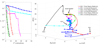 |
Fig. 3 Convergence history of the Trust Region Reflective and the Levenberg-Marquardt algorithms for the iterative solution of the nonlinear least-squares problem (9) for three different initial guesses. Left panel: sum of squared residuals, S, given by Eq. (8) as a function of the number of forward map, F, evaluations. The horizontal dashed line represents the tolerance of 10−6. Right panel: sequence of improving approximate solutions in the 3D space spanned by the (height-independent) magnetic field parameters [B, θB,χB]. |
5 Numerical setup
The solution strategy outlined in Sects. 3 and 4 has been implemented as a MATLAB (MATLAB 2023) routine. As a first application, we considered the inversion of the emergent Stokes profiles of the Ca I line at 4227 Å, which are produced by the transition between the ground level of neutral calcium (4s2 1S0) and the excited level 4s4p 1Po1. The Ca I 4227 polarization profiles can be suitably modeled by considering a two-level atomic model. The line-core scattering polarization signal constitutes an important observable for probing the low-chromosphere magnetic fields via the Hanle effect (Stenflo 1982; Faurobert-Scholl 1992), while the scattering polarization wing lobes are sensitive to photospheric magnetic fields via magneto-optical effects (e.g., Alsina Ballester et al. 2018).
For the forward problem, we discretized the wavelength interval [4219 Å, 4234 Å] with 101 points. In the angular dimensions, we used 7 points uniformly distributed in the azimuth and two sets of 4 points for μ, resulting in a total of NΩ = 56 points. We considered the FAL-C atmospheric model in the height interval [−100 km, 1860 km], which is discretized with Nz = 35 points. For the formal solution, we used the DELO-linear exponential integrator and a linear conversion to optical depth (see Janett et al. 2017; D’Anna et al. 2024). We set the tolerance of the preconditioned GMRES solver to 10−6. Our forward engine incorporates both the general angle-dependent description of PRD effects and the angle-averaged approximation. Considering the Ca I 4227 line, a single iterative solution of the 1D forward non-LTE problem (Nz = 35, NΩ = 56, and Nν = 101) requires approximately 10 processor minutes (@2.50 GHz) for the angledependent PRD case and less than 1 processor minute for the angle-averaged PRD case. To substantially reduce the overall computational cost, unless otherwise specified, we present results obtained using the angle-averaged approximation.
In this section, we assess the choice of the optimization solver and the adopted approximation for the Jacobian. As testcase, we considered the Ca I 4227 Stokes fractional profiles at μ = 0.07 synthesized in the static FAL-C atmosphere with a horizontal height-independent magnetic field [B,θB,χB] = [20, π/2,0]. For the height-independent case, it is sufficient to consider a single node for each atmospheric fit quantity. Moreover, we used along the whole paper the following hard constraints on the magnetic field fit parameters 0 < B < 200 G, 0 < θB < π, and -π < χB < π.
5.1 Assessment of optimization solvers
For the optimization solver, we employed the Matlab minimization routine lsqcurvefit, by adopting its default convergence criteria. This routine requires a user-defined function to compute the vector-valued forward map Iout(x), enabling a direct implementation of the forward engine in the optimization solver. In these tests, we use the approximated Jacobian, J, described in Sect. 4.4; we refer to Sect. 5.2 for its assessment. The left panel of Fig. 3 shows an example of the convergence history for the two minimization algorithms: the Trust Region Reflective and Levenberg-Marquardt. For added generality, we initiated the inversion process with three distinct initial guesses for the magnetic field, namely: IG-1: x0 = [1,π∕4, π∕2], IG-2: x0 = [10,π∕2,0], and IG-3: x0 = [10,3π∕4, -π∕2].
The Trust Region Reflective method clearly outperforms the Levenberg-Marquardt method in terms of the number of forward map evaluations required to reach convergence. The right panel of Fig. 3 provides an explicit visualization of the path to the solution, illustrating the sequence of improving approximate solutions in the 3D space spanned by the (height-independent) magnetic field parameters for the three different initial guesses.
The Trust Region Reflective method is able to find a more direct path in the 3D parameter space toward the desired solution. In contrast, the Levenberg–Marquardt algorithm slows down significantly, even failing to converge when the initial guess is far from the solution (see IG-2 and IG-3), and it gets stuck in a local minimum. We attribute this to the highly corrugated structure of the metric S hypersurface, see Eq. (8), which is a consequence of the ambiguities that arise when the polarization profiles result from the joint action of scattering processes, and of the Zeeman and Hanle effects (e.g., Asensio Ramos et al. 2008). In conclusion, we did not use the Levenberg-Marquardt for inverting the magnetic field when considering scattering polarization.
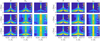 |
Fig. 4 Numerical approximation of Eq. (11) for Q/I (left panels) and U/I (right panels) at μ = 0.07, sampled on the FAL-C spatial grid and plotted in log10(J) scale. Derivatives are computed w.r.t. magnetic field parameters (see titles on each column) for the reference accurate Jacobian (first row), the single-GMRES (second row), and the double-GMRES (third row) approximations. |
5.2 Assessment of the approximate Jacobian
In Fig. 4, we compare different numerical approximations of the Jacobian, see Eq. (12), of emergent Q/I and U/I at μ = 0.07, computed w.r.t. the magnetic field parameters [B, θB,χB] at the Nz = 45 spatial points of the forward problem grid, that is for the case with q = x, see Eq. (7). Although this is not the actual Jacobian used in the (usually node-based) inversion problem, its visualization provides valuable insights into both the accuracy of our approximated Jacobian and the response function of the Ca I 4227 to the magnetic field. In particular, Fig. 4 presents a comparison between the accurate reference Jacobian, computed evaluating the forward map with tol = 10−10 (top row), and the approximated Jacobian described in Sect. 4.4, obtained using a single additional GMRES iteration (single-GMRES; middle row). For comparison, we also show the approximated Jacobian obtained using two additional GMRES iterations (double-GMRES; bottom row). For all calculations of J we adopted the step sizes δB = 0.5 G, δθB = δχB = 0.5 degrees. We also tested halved and double values of these step sizes, but the adopted values revealed sufficiently small to validate the first-order perturbation assumption, yet large enough to dominate the numerical noise in the forward map calculation. Notably, our approximation successfully captures the primary features of the Jacobian related to the Hanle and magneto-optical effects. The main artifacts are primarily confined to the lowest and highest regions of the atmospheric model, which are known to have a negligible impact on the emergent signal.
Furthermore, we assessed the performance of three different numerical approximations of the Jacobian (single-GMRES, double-GMRES, and the Matlab lsqcurvefit solver-default)5 in the node-based inversion process. Notably, the use of the single-GMRES or double-GMRES approximations required an equal or lower number of iterations to reach convergence w.r.t. the use of the solver-default Jacobian in all test cases, reducing the time-to-solution of a factor up to 5. Moreover, we have tested the calculation of the Jacobian using both forward differences and central differences. Since we did not find significant differences between the Jacobians retrieved by the two finite difference methods, we opt for the more cost-effective (halved cost) forward differences throughout this paper.
6 Inversion results
In this section, we fit the vector magnetic field to the fractional polarization profiles of Ca I 4227 at μ = 0.07 synthesized in different 1D plane-parallel solar atmospheric models. A depth-stratified 1D atmosphere proved to be sophisticated enough to satisfactorily model the polarization signals of the Ca I line at 4227 Å (e.g., Capozzi et al. 2022). The reference direction for positive Stokes Q is taken parallel to the limb, which corresponds to the x-axis. The magnetic field vector is specified by the intensity B, the inclination θB with respect to the vertical, and the azimuth χB measured on the x - y plane, counter-clockwise (for an observer at z > 0) from the x-axis.
6.1 Height-dependent magnetic field
As a first height-dependent test-case, we considered the static FAL-C atmosphere with a magnetic field [B(z), θB(z),χB(z)] that varies linearly with the height z, as shown in the left column of Fig. 5 (see blue lines). We employed a two-cycle inversion technique: in the first cycle, we started with an initial guess using a single node for each magnetic field parameter. We then adopted the solution of the first cycle as initial guess for the second cycle, where we used two nodes, placed at heights of 600 km and 900 km, for each magnetic field parameter and a linear interpolation (and extrapolation) to obtain the magnetic field parameters on the forward problem spatial grid, as described in Eq. (7)6. We found that this two-cycles approach greatly improved the convergence of the inversion. A single inversion cycle required around 10 optimization algorithm iterations to reach the target tolerance. Each inversion process took around 1 processor hour (@2.50 GHz).
To test the robustness against different initializations, we started the inversion process with two different initial guesses: IG-1: x0 = [10,π∕4,0] and IG-2: x0 = [10, 3π∕4,0]. The inversion results are presented in Fig. 5, which shows the original model and the fitted magnetic field parameters (left column), and the synthetic input and retrieved fractional polarization profiles (right column). For both initial guesses, the Stokes profiles retrieved by the inversion process are in excellent agreement with the input ones. By contrast, the fitted height-dependent magnetic field parameters, and especially the inclination θB, depend on the initial guess. In particular, we note that the heightdependent inclination θB obtained starting with IG-2 is nearly the supplementary angle w.r.t. the original one. This explicitly shows that there are different magnetic field configurations that lead to similar scattering (and Zeeman) polarization signals. We thus observe that even when adopting a cycle-based approach, the magnetic-inversion method can retrieve multiple satisfactory solutions.
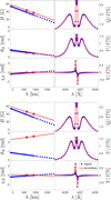 |
Fig. 5 Inversion of Ca I 4227 fractional Stokes profiles at μ = 0.07 synthesized in the static FAL-C model in the presence of a heightdependent magnetic field for two different initial guesses: IG-1 (top panel) and IG-2 (bottom panel). Left column: magnetic field magnitude, B, inclination, θB, and azimuth, χB of the original model (blue dots) and two-nodes fitted (red lines) quantities. Right column: synthetic input Iobs (blue dots), and retrieved Iout (red lines), fractional polarization Q/I, U/I, and V/I profiles. |
6.2 Height-dependent magnetic and bulk velocity fields
We now add the ingredient of bulk velocities. Although the inversion engine is able to consider arbitrary bulk velocity fields, we hereafter consider only vertical bulk velocities for simplicity. For this test, we consider two different vertical columns extracted from a snapshot of the 3D MHD simulation of the solar atmosphere by Carlsson et al. (2016), corresponding to model A and model D analyzed by Guerreiro et al. (2024). Such columns have a vertical resolution of 20 km for the height interval [zmin, zmax] = [−100 km, 1400 km], which fully includes the formation region of the line. The Bifrost atmospheric model provides temperature, electron and proton number density, vertical bulk velocity, magnetic field vector, and the hydrogen populations at each height point. Microturbulence adopted from Fontenla et al. (1991) is included. We fit the model atmospheres A and D with a three-cycle approach. First, we only fit the vertical bulk velocity field to the intensity profile, assuming a zero magnetic field. Second, keeping fixed the bulk velocity from the first cycle, we fit a height-independent magnetic field to the fractional Stokes profiles. Third, we use the output of the second cycle as initial guess for the third cycle, where we fit a height-dependent magnetic field to the fractional Stokes profiles. We note that with this approach we are fitting bulk velocities to the intensity spectrum only.
More precisely, during the first cycle we only fit the vertical bulk velocity field to the intensity profile I, while considering the input thermal stratification of the atmosphere fixed. In this cycle, we used 4 nodes interpolated with the shape-preserving piecewise cubic method, starting with a zero initial guess x0 = [0, 0, 0, 0]. Such nodes are placed at heights of 200 km, 400 km, 750 km, and 850 km for model A and 50 km, 200 km, 600 km, and 700 km for model D, and the inversion results are respectively presented in the top panels of Fig. 6. The inversion process provides a good agreement between the retrieved intensity profiles and the synthetic input values for both atmospheric models. Furthermore, the fitted bulk velocity field is a good estimate of the original one. In the second cycle, we fit the vector magnetic field to the Q∕I, U∕I, and V/I profiles, using a single node for each magnetic field parameter with the initial guess x0 = [10, π/2,0]. We then adopt the fitted magnetic field of the second cycle as initial guess for the third cycle, using two linearly interpolated nodes, placed at heights of 200 km and 600 km for model A and 200 km and 650 km for model D. The inversion results are presented in the middle (one-node) and bottom (two-node) panels of Fig. 6.
The inversion process yields excellent agreement between the retrieved Stokes profiles and the input synthetic values for both atmospheric models. Furthermore, the two-nodes fitted magnetic field provides a reasonably accurate estimate of the original magnetic field. However, the accuracy of the inversion process is contingent upon the number of nodes, their spatial distribution, and the choice of interpolant. A comprehensive examination of these factors is warranted to fully understand their impact on the inversion process, and this topic deserves a dedicated investigation.
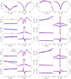 |
Fig. 6 Inversion of Ca I 4227 fractional Stokes profiles at µ = 0.07 synthesized in two different vertical columns of a Bifrost model labeled in Guerreiro et al. (2024) as Model A (left panels) and Model D (right panels), in the presence of a height-dependent vertical bulk velocity and magnetic fields. Top panels: fitting of the vertical bulk velocity field to the intensity profile. Left columns: vertical bulk velocity field vz of the original model (blue dots) and four-nodes fitted (red lines) quantities. Right columns: synthetic input (blue dots) and retrieved (red lines) intensity profiles. Middle and bottom panels: fitting of the magnetic field to the fractional Stokes profiles, exploiting one single node (middle panels) and two nodes (bottom panels). Left columns: magnetic field magnitude, B, inclination, θB, and azimuth, χB of the original model (blue line) and fitted (red circles) quantities. Right columns: synthetic input Iobs (blue line) and retrieved Iout (red circles) fractional polarization Q/I, U/I, and V/I profiles. |
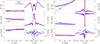 |
Fig. 7 Same as Fig. 6, but with the addition of wavelength-dependent Gaussian noise to the synthetic Stokes profiles. |
6.3 Including photon noise
In contrast to our previous calculations, we now account for photon noise in the synthetic input Stokes profiles. We assume photon noise to be additive, Gaussian, and wavelength-dependent, namely,
 (13)
(13)
where In-lessi is the noiseless synthetic input, N(0,1) represents a standard normal distribution (with mean zero and standard deviation one), and σni is the noise amplitude which is proportional to the square root of the intensity signal. We assumed a signal-to-noise ratio of 1000 in the continuum Ic, leading to
 (13)
(13)
where Ii is the noiseless intensity at the wavelength corresponding to index i. According to the analysis by Díaz Baso et al. (2025), this noise level is expected for Ca I 4227 observations at a 4-m telescope, with pixel size of 0.05 arcseconds, exposure of seconds, and spectral binning of 20 mÅ.
We repeated the inversions presented in Sect. 6.2 considering profiles that include added noise. At this noise level, the Q/I and U/I structures persist, whereas the V/I signal is degraded to the point of being indistinguishable from the noise. As shown in Fig. 7, the inversion results demonstrate a good degree of consistency between the retrieved Stokes profiles and the input synthetic values for both atmospheric models. Moreover, the fitted vector magnetic fields, with and without noise, exhibit a decent agreement, suggesting that the inversion process is reasonably robust to the presence of noise. We surmise that this is because Q/I and U/I provide substantial information about the vector magnetic field.
6.4 Considering angle-dependent PRD effects
We report the successful inversion of Ca I 4227 fractional Stokes profiles synthesized at μ = 0.07 in the static FAL-C model, in the presence of a height-independent magnetic field with parameters [B,θB,χB] = [20, π/2,0], considering the general angle-dependent description of PRD effects to obtain the synthetic Iobs. For the inversion, we used the initial guess for the magnetic field x0 = [10,3π/4, -π/2].
We performed the inversion by considering both the angledependent and the angle-averaged descriptions of PRD effects. Our inversion process required 7 iterations to reach convergence, and it took approximately 3 processor hours (@2.50 GHz) for the angle-dependent case, while it took 14 iterations and 1.3 processor hour (@2.50 GHz) for the angle-averaged case. The inversion results are presented in Fig. 8. To the best of our knowledge, this represents the first-ever spectropolarimetric inversion that incorporates scattering polarization with the general angle-dependent description of PRD effects. Notably, the fitted vector magnetic field and the retrieved Stokes profiles are in excellent agreement with the original and synthetic values both for angle-dependent and the angle-averaged inversions. This seems to suggest that, despite introducing artifacts in the line-core polarization, the angle-averaged description of PRD could be suitable to fit the magnetic field to the observed fractional Stokes profiles. This topic deserves a dedicated investigation.
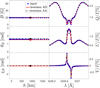 |
Fig. 8 Same as Fig. 5 but in the presence of the height-independent magnetic field [B,θB,χB] = [20, π/2,0] and considering the angledependent description of PRD to obtain the synthetic input Iobs. The inversion is performed by considering the angle-dependent (AD; red lines) and the angle-averaged (AA; black lines) descriptions of PRD. |
7 Conclusions
In this paper, we have presented a new inversion approach to fit the vector magnetic field to the Stokes profiles of strong solar resonance lines accounting for PRD, scattering polarization, and the Hanle and Zeeman effects. We tested this approach inverting spectropolarimetric profiles of the Ca I line at 4227 Å synthesized in 1D plane-parallel solar atmospheric models.
We proposed and tested an approximate way for computing the Jacobian required for the optimization solver at each iteration step, which allowed us to reduce the time-to-solution by up to a factor of 5. We also showed that, for this problem, the Trust Region Reflective optimization solver clearly outperforms the Levenberg-Marquardt one. The Trust Region Reflective algorithm is indeed able to follow the negative curvature of the loss function, finding a smoother path in the parameter space toward the solution. The inversion of Stokes profiles provided a good estimate of the original magnetic field, both in semi-empirical atmospheric models and in vertical columns of a 3D MHD simulation. Furthermore, we have investigated the impact of adding photon noise to the input data, finding that the inversion process is reasonably robust to its presence. We also successfully performed the first-ever spectropolarimetric inversion that incorporates scattering polarization with the general angle-dependent description of PRD.
In conclusion, we demonstrated the potential of our inversion approach for retrieving the vector magnetic field from strong resonance lines that exhibit scattering polarization and are sensitive to Hanle and Zeeman effects. Ongoing developments include the uncertainty estimate of atmospheric fit parameters, either from the Jacobian (del Toro Iniesta & Ruiz Cobo 2016) or through Monte Carlo or bootstrap methods (e.g., Press et al. 2007). Possible applications of this inversion approach include a range of exciting new spectropolarimetric observations from the ViSP instrument at DKIST (Rimmele et al. 2020; Rast et al. 2021), the series of CLASP sounding rocket experiments (Kano et al. 2017; Rachmeler et al. 2022) and future space missions.
Acknowledgements
We acknowledge stimulating discussions with Dr. Tanausú del Pino Alemán and Dr. Pietro Benedusi. We also thank the anonymous referee for the careful reading of the manuscript. The financial support by the Swiss National Science Foundation (SNSF) through grant 231308 is gratefully acknowledged. IM acknowledges the financial support from the Serbian Ministry of Science and Technology through the grants 451-03-136/2025-03/200104 and 451-03-136/2025-03/200002.
References
- Alsina Ballester, E., Belluzzi, L., & Trujillo Bueno, J. 2018, ApJ, 854, 150 [Google Scholar]
- Asensio Ramos, A., Trujillo Bueno, J., & Landi Degl’Innocenti, E. 2008, ApJ, 683, 542 [Google Scholar]
- Benedusi, P., Janett, G., Riva, G., Belluzzi, L., & Krause, R. 2022, A&A, 664, A197 [NASA ADS] [CrossRef] [EDP Sciences] [Google Scholar]
- Björck, A. 1996, Numerical Methods for Least Squares Problems (Society for Industrial and Applied Mathematics) [Google Scholar]
- Bommier, V. 1997a, A&A, 328, 706 [NASA ADS] [Google Scholar]
- Bommier, V. 1997b, A&A, 328, 726 [NASA ADS] [Google Scholar]
- Capozzi, E., Alsina Ballester, E., Belluzzi, L., & Trujillo Bueno, J. 2022, A&A, 657, A44 [NASA ADS] [CrossRef] [EDP Sciences] [Google Scholar]
- Carlsson, M., Hansteen, V. H., Gudiksen, B. V., Leenaarts, J., & De Pontieu, B. 2016, A&A, 585, A4 [NASA ADS] [CrossRef] [EDP Sciences] [Google Scholar]
- Carlsson, M., De Pontieu, B., & Hansteen, V. H. 2019, ARA&A, 57, 189 [Google Scholar]
- Coleman, T. F., &Li, Y. 1996, SIAM J. Optim., 6, 418 [Google Scholar]
- D’Anna, M., Janett, G., & Belluzzi, L. 2024, A&A, 689, A90 [NASA ADS] [CrossRef] [EDP Sciences] [Google Scholar]
- de la Cruz Rodríguez, J., & van Noort, M. 2017, Space Sci. Rev., 210, 109 [Google Scholar]
- de la Cruz Rodríguez, J., Leenaarts, J., Danilovic, S., & Uitenbroek, H. 2019, A&A, 623, A74 [Google Scholar]
- De Pontieu, B., Polito, V., Hansteen, V., et al. 2021, Sol. Phys., 296, 84 [NASA ADS] [CrossRef] [Google Scholar]
- del Toro Iniesta, J. C., & Ruiz Cobo, B. 2016, Living Rev. Sol. Phys., 13, 4 [Google Scholar]
- Díaz Baso, C. J., Milic´, I., Rouppe van der Voort, L., & Schlichenmaier, R. 2025, A&A, 693, A272 [NASA ADS] [CrossRef] [EDP Sciences] [Google Scholar]
- Faurobert-Scholl, M. 1992, A&A, 258, 521 [NASA ADS] [Google Scholar]
- Fontenla, J. M., Avrett, E. H., & Loeser, R. 1991, ApJ, 377, 712 [NASA ADS] [CrossRef] [Google Scholar]
- Guerreiro, N., Janett, G., Riva, S., Benedusi, P., & Belluzzi, L. 2024, A&A, 683, A207 [NASA ADS] [CrossRef] [EDP Sciences] [Google Scholar]
- Janett, G., Carlin, E. S., Steiner, O., & Belluzzi, L. 2017, ApJ, 840, 107 [NASA ADS] [CrossRef] [Google Scholar]
- Janett, G., Benedusi, P., Belluzzi, L., & Krause, R. 2021, A&A, 655, A87 [NASA ADS] [CrossRef] [EDP Sciences] [Google Scholar]
- Janett, G., Benedusi, P., & Riva, F. 2024, A&A, 682, A68 [NASA ADS] [CrossRef] [EDP Sciences] [Google Scholar]
- Kano, R., Trujillo Bueno, J., Winebarger, A., et al. 2017, ApJ, 839, L10 [NASA ADS] [CrossRef] [Google Scholar]
- Landi Degl’Innocenti, E., & Landolfi, M. 2004, Astrophysics and Space Science Library, 307, Polarization in Spectral Lines (Dordrecht: Kluwer Academic Publishers) [Google Scholar]
- Li, H., del Pino Alemán, T., Trujillo Bueno, J., & Casini, R. 2022, ApJ, 933, 145 [NASA ADS] [CrossRef] [Google Scholar]
- Li, H., del Pino Alemán, T., Trujillo Bueno, J., et al. 2023, ApJ, 945, 144 [Google Scholar]
- Li, H., del Pino Alemán, T., & Trujillo Bueno, J. 2024, ApJ, 975, 110 [Google Scholar]
- Martínez González, M. J., Collados, M., & Ruiz Cobo, B. 2006, A&A, 456, 1159 [NASA ADS] [CrossRef] [EDP Sciences] [Google Scholar]
- MATLAB 2023, version 9.14.0 (R2023a), (Natick, Massachusetts: The MathWorks Inc.) [Google Scholar]
- Milic´, I., & Faurobert, M. 2012, A&A, 547, A38 [NASA ADS] [CrossRef] [EDP Sciences] [Google Scholar]
- Milic´, I., & van Noort, M. 2018, A&A, 617, A24 [Google Scholar]
- Moré, J. J. 1978, in Lecture Notes in Mathematics, 630 (Berlin Springer Verlag), 105 [Google Scholar]
- Nocedal, J., & Wright, S. J., eds. 1999, Trust-Region Methods (New York, NY: Springer New York), 64 [Google Scholar]
- Press, W. H., Teukolsky, S. A., Vetterling, W. T., & Flannery, B. P. 2007, Numerical Recipes, 3rd edn.: The Art of Scientific Computing (Cambridge University Press) [Google Scholar]
- Rachmeler, L. A., Trujillo Bueno, J., McKenzie, D. E., et al. 2022, ApJ, 936, 67 [NASA ADS] [CrossRef] [Google Scholar]
- Rast, M. P., Bello González, N., Bellot Rubio, L., et al. 2021, Sol. Phys., 296, 70 [NASA ADS] [CrossRef] [Google Scholar]
- Rees, D. E., & Saliba, G. J. 1982, A&A, 115, 1 [NASA ADS] [Google Scholar]
- Rimmele, T. R., Warner, M., Keil, S. L., et al. 2020, Sol. Phys., 295, 172 [Google Scholar]
- Riva, F., Janett, G., Belluzzi, L., et al. 2025, A&A, 699, A233 [NASA ADS] [CrossRef] [EDP Sciences] [Google Scholar]
- Ruiz Cobo, B., & del Toro Iniesta, J. C. 1992, ApJ, 398, 375 [Google Scholar]
- Stenflo, J. O. 1982, Sol. Phys., 80, 209 [Google Scholar]
- Šteˇpán, J., del Pino Alemán, T., & Trujillo Bueno, J. 2022, A&A, 659, A137 [NASA ADS] [CrossRef] [EDP Sciences] [Google Scholar]
- Trujillo Bueno, J., & del Pino Alemán, T. 2022, ARA&A, 60, 415 [NASA ADS] [CrossRef] [Google Scholar]
The residuals are often weighted by the inverse of the measurement uncertainty (or other factors) that additionally weight specific Stokes components of interest (e.g., del Toro Iniesta & Ruiz Cobo 2016).
Meaning that the forward map Iout depends non-linearly on x.
We note that STiC and HanleRT-TIC enhance their Levenberg-Marquardt algorithm by incorporating the back-tracking technique at each iteration (see Press et al. 2007).
The lsqcurvefit solver-default algorithm computes J through forward finite differences, using a step size of 1.5 · 10−8.
All Figures
|
Fig. 1 Schematic representation of the forward non-LTE RT problem, that is, the iterative solution to determine the emergent Stokes profiles, Iout, when provided a set of atmospheric parameters, q. |
| In the text | |
|
Fig. 2 Schematic representation of the inversion problem, that is the iterative solution to determine the atmospheric parameters, qout, that best reproduce an observed Stokes spectrum, Iobs. |
| In the text | |
|
Fig. 3 Convergence history of the Trust Region Reflective and the Levenberg-Marquardt algorithms for the iterative solution of the nonlinear least-squares problem (9) for three different initial guesses. Left panel: sum of squared residuals, S, given by Eq. (8) as a function of the number of forward map, F, evaluations. The horizontal dashed line represents the tolerance of 10−6. Right panel: sequence of improving approximate solutions in the 3D space spanned by the (height-independent) magnetic field parameters [B, θB,χB]. |
| In the text | |
|
Fig. 4 Numerical approximation of Eq. (11) for Q/I (left panels) and U/I (right panels) at μ = 0.07, sampled on the FAL-C spatial grid and plotted in log10(J) scale. Derivatives are computed w.r.t. magnetic field parameters (see titles on each column) for the reference accurate Jacobian (first row), the single-GMRES (second row), and the double-GMRES (third row) approximations. |
| In the text | |
|
Fig. 5 Inversion of Ca I 4227 fractional Stokes profiles at μ = 0.07 synthesized in the static FAL-C model in the presence of a heightdependent magnetic field for two different initial guesses: IG-1 (top panel) and IG-2 (bottom panel). Left column: magnetic field magnitude, B, inclination, θB, and azimuth, χB of the original model (blue dots) and two-nodes fitted (red lines) quantities. Right column: synthetic input Iobs (blue dots), and retrieved Iout (red lines), fractional polarization Q/I, U/I, and V/I profiles. |
| In the text | |
|
Fig. 6 Inversion of Ca I 4227 fractional Stokes profiles at µ = 0.07 synthesized in two different vertical columns of a Bifrost model labeled in Guerreiro et al. (2024) as Model A (left panels) and Model D (right panels), in the presence of a height-dependent vertical bulk velocity and magnetic fields. Top panels: fitting of the vertical bulk velocity field to the intensity profile. Left columns: vertical bulk velocity field vz of the original model (blue dots) and four-nodes fitted (red lines) quantities. Right columns: synthetic input (blue dots) and retrieved (red lines) intensity profiles. Middle and bottom panels: fitting of the magnetic field to the fractional Stokes profiles, exploiting one single node (middle panels) and two nodes (bottom panels). Left columns: magnetic field magnitude, B, inclination, θB, and azimuth, χB of the original model (blue line) and fitted (red circles) quantities. Right columns: synthetic input Iobs (blue line) and retrieved Iout (red circles) fractional polarization Q/I, U/I, and V/I profiles. |
| In the text | |
|
Fig. 7 Same as Fig. 6, but with the addition of wavelength-dependent Gaussian noise to the synthetic Stokes profiles. |
| In the text | |
|
Fig. 8 Same as Fig. 5 but in the presence of the height-independent magnetic field [B,θB,χB] = [20, π/2,0] and considering the angledependent description of PRD to obtain the synthetic input Iobs. The inversion is performed by considering the angle-dependent (AD; red lines) and the angle-averaged (AA; black lines) descriptions of PRD. |
| In the text | |
Current usage metrics show cumulative count of Article Views (full-text article views including HTML views, PDF and ePub downloads, according to the available data) and Abstracts Views on Vision4Press platform.
Data correspond to usage on the plateform after 2015. The current usage metrics is available 48-96 hours after online publication and is updated daily on week days.
Initial download of the metrics may take a while.