| Issue |
A&A
Volume 701, September 2025
|
|
|---|---|---|
| Article Number | A256 | |
| Number of page(s) | 3 | |
| Section | Extragalactic astronomy | |
| DOI | https://doi.org/10.1051/0004-6361/202555988 | |
| Published online | 18 September 2025 | |
Redshift ∼2.7 is not special
Comment on the Kolmogorov analysis of JWST deep survey galaxies
Indian Institute of Astrophysics, Bangalore 560034, India
⋆ Corresponding author: This email address is being protected from spambots. You need JavaScript enabled to view it.
Received:
17
June
2025
Accepted:
17
July
2025
Abstract
Galikyan et al. (2025, A&A, 696, L21) reported a statistically significant change in galaxy spectral properties at redshift z ≃ 2.7 based on a Kolmogorov Stochasticity Parameter analysis of JWST spectroscopic data of galaxies. In this comment, we demonstrate that this result is critically driven by a single outlier in the dataset that was employed. This outlier arises from the use of a questionable redshift estimate for one spectrum. When the outlier is removed or the redshift is corrected, the claimed transition at z ≃ 2.7 disappears entirely. By independently reproducing the previous analysis, we demonstrate that the claimed feature is not a robust statistical signal, but an artefact of this anomalous data point.
Key words: methods: data analysis / methods: statistical / galaxies: high-redshift
© The Authors 2025
 Open Access article, published by EDP Sciences, under the terms of the Creative Commons Attribution License (https://creativecommons.org/licenses/by/4.0), which permits unrestricted use, distribution, and reproduction in any medium, provided the original work is properly cited.
This article is published in open access under the Subscribe to Open model. This email address is being protected from spambots. You need JavaScript enabled to view it. to support open access publication.
1. Introduction
Galikyan et al. 2025 (hereafter, G25) analyses JWST spectroscopic data of galaxies published by Price et al. (2025) in order to check for changes in the spectral properties of the sample galaxies with redshift. They selected galaxy spectra with redshift (z) quality flags marked as either ‘secure’ or ‘solid’ in the dataset derived from the Ultradeep NIRSpec and NIRCam ObserVations before the Epoch of Reionization (UNCOVER) Cycle 1 Treasury survey (Bezanson et al. 2024). They imposed an additional selection criterion that the spectral peak be close to 656 nm in the rest frame. From this subset, the authors identified the observed-frame wavelengths (λobs) corresponding to the spectral peaks and converted them to the rest frame (λrest) using the redshift values estimated by Price et al. (2025). They then grouped the data into small redshift bins and computed the Kolmogorov stochasticity parameter (KSP) for the set of rest-frame peak wavelengths within each bin. From examination of how the KSP values varied with redshift, the authors of G25 report a statistically significant change in spectral properties at z ≃ 2.7, claiming a confidence level exceeding 99%.
A sudden transition in galaxy spectral properties at z ≃ 2.7 is of significant astrophysical interest. Motivated by this claim, we revisited the JWST spectroscopic dataset to investigate the origin of the reported feature. As part of this effort, we reproduced the analysis carried out in G25. In doing so, we found that the reported change in spectral properties at z ≃ 2.7 arises entirely from the inclusion of a single outlier in their dataset. We detail our findings in the following section.
2. Re-analysis of G25
Using rest-frame peak wavelengths in JWST galaxy spectra, the authors of G25 computed KSP values. Specifically, they selected peaks near 656 nm, where the Hα emission line is typically prominent. They interpreted KSP values thus computed as a measure of the degree of randomness in spectra and reported a statistically significant transition in the KSP distribution at z ≃ 2.7. It is unclear how an analysis based solely on a single wavelength feature meaningfully captures the overall randomness of galaxy spectra. Additionally, the authors of G25 implicitly assumed a uniform spectroscopic targeting strategy across all redshifts in the UNCOVER dataset. In practice, the source selection criteria varied significantly with redshift (Price et al. 2025), introducing redshift-dependent biases. A further assumption underlying their analysis is that the Hα emission line remains the dominant spectral feature across all redshifts. This is not generally valid, as galaxies at higher redshifts often exhibit stronger [O III] emission than Hα. Nonetheless, accepting their methodology for the sake of argument, we independently reproduced their analysis using the same UNCOVER sample. Our re-analysis demonstrates that the reported transition at z ≃ 2.7 arises entirely from the inclusion of a single outlier in their sample.
This outlier is visible in Figure 1 of G25 near ∼0.634 μm. We have reproduced their figure following their described methodology (see Fig. 1), highlighting the outlier in orange1. Upon examining the corresponding data point (λobs = 2.184 μm) in the publicly available dataset from Price et al. (2025), we found that the relevant spectrum has four different redshift estimates: 2.444 (z_spec), 2.324 (z_spec16), 2.328 (z_spec50), and 2.331 (z_spec84). We note that the outlier arises only when using the z_spec value to convert λobs. If any of the alternative redshift estimates are used, the corresponding rest-frame wavelength falls well within the general distribution of the other data points in Fig. 1. This suggests that the z_spec value is likely a misestimate for the corresponding spectrum and that one of the alternative values – which are remarkably consistent with one another – should be preferred. Moreover, visual inspection of the spectrum (see Fig. 3) confirms that the observed Hα emission line lies close to the expected rest-frame wavelength when using any of the alternative redshift estimates (see Fig. 4).
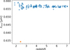 |
Fig. 1. Rest-frame peak wavelengths near 656 nm in JWST galaxy spectra, as used in G25 in the authors’ analysis. The outlier, clearly offset from the rest of the distribution, is highlighted in orange. |
It is important to note that wavelength calibration uncertainties in JWST/NIRSpec spectra, particularly in the low-resolution prism mode, can impact the accuracy of redshift estimates (Ferruit et al. 2022; de Graaff et al. 2025; D’Eugenio et al. 2025). The prism mode suffers from reduced spectral resolution at shorter wavelengths (R ≃ 30 at ∼1 μm compared to R ≃ 300 at ∼5 μm), making it more difficult to obtain precise redshifts at lower z (Jakobsen et al. 2022). In the case of the outlier spectrum discussed here, the large discrepancy in the z_spec value relative to the other redshift estimates (∼5% difference) combined with visual confirmation of the Hα line position may point to an error likely exceeding the expected calibration uncertainties.
To demonstrate the influence of the outlier in the analysis in G25, we used a sliding window (bin), with each containing 20 λrest values sorted by redshift, and computed the KSP for the values in each bin. We adopted the standard normal distribution as the reference theoretical distribution. The resulting plot of KSP versus redshift based on the same data used in G25 is shown in Fig. 2a.
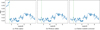 |
Fig. 2. Kolmogorov stochasticity parameter versus redshift for the dataset used in G25 under different treatments of the outlier. (a) KSP computed with the outlier. (b) KSP computed with the outlier excluded. (c) KSP computed with the outlier redshift corrected using z_spec50. In all panels, the vertical dashed line marks z = 2.7. |
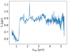 |
Fig. 3. Spectrum from JWST corresponding to the outlier data point, shown in observed wavelengths. The redshifted Hα emission line peak is clearly visible at ∼2.2 μm. |
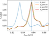 |
Fig. 4. Region around the Hα emission line in the spectrum corresponding to the outlier data point. The observed wavelength (λobs) has been converted to the rest frame (λrest) using different redshift estimates: the blue curve uses z_spec, while the orange, green, and red curves correspond to z_spec16, z_spec50, and z_spec84, respectively. The vertical line marks λrest = 656.46 nm. |
Figure 2a differs from Figure 2 of G25 in two main respects: the number of data points and the spread of KSP values. The difference in the number of points arises because the authors of G25 used 1000 randomly generated, overlapping redshift bins of varying sizes, while we used a uniform sliding bin of size 20. The difference in the spread of KSP values stems from their use of a generalised normal distribution with a free sharpness parameter fitted independently in each redshift bin. In contrast, we used a fixed standard normal distribution across all bins. Despite these methodological differences, our Fig. 2a successfully reproduces the sharp change in KSP around z ≃ 2.7 in Figure 2 of G25, along with other observed trends.
When the outlier is excluded from the analysis, this significant jump in KSP disappears entirely (see Fig. 2b). The same result holds when the outlier’s redshift is replaced with any of the alternative estimates discussed earlier (see Fig. 2c). This demonstrates that the claimed change in KSP is entirely driven by a single inconsistent data point.
3. Summary
The recent work of G25 analyses JWST spectra from Price et al. (2025). The authors selected spectra with high-confidence redshift estimates and those with peaks near 656 nm in the rest frame. They examined how the degree of randomness in the rest-frame peak wavelengths varied with redshift and report a statistically significant change in spectral properties at z ≃ 2.7.
We show that their result is critically dependent on a single outlier in their dataset. This outlier, visible in their own Figure 1, arises from the choice of one specific redshift estimate out of several available for a given spectrum. When any of the alternative redshift estimates are used, the corresponding rest-frame wavelength no longer deviates from the overall distribution.
We have independently reproduced the KSP versus redshift trend and confirm that the reported feature at z ≃ 2.7 can be replicated – but only when the outlier is included. Once excluded or corrected, the jump in KSP disappears. This demonstrates that the claimed transition is not a robust statistical feature but an artefact of a single inconsistent data point.
The Python scripts used in this work can be accessed at https://github.com/prajwel/no_special_redshift
Acknowledgments
We thank the anonymous reviewer for their constructive comments and helpful suggestions, which have improved this article. This work is based on a talk presented at a journal club meeting at the Indian Institute of Astrophysics. The author is grateful to Koshy George and C. S. Stalin for insightful discussions. Thanks are also due to Norayr Galikyan for responding to queries related to their work. Astropy, IPython, Matplotlib, NumPy, and Scipy were used for data analysis, viewing, and plotting (Astropy Collaboration 2013); astropy:2018; astropy:2022; matplotlib; numpy; ipython2007; 2020SciPy-NMeth. This work is based on observations made with the NASA/ESA/CSA James Webb Space Telescope. The data were obtained from the Mikulski Archive for Space Telescopes at the Space Telescope Science Institute, which is operated by the Association of Universities for Research in Astronomy, Inc., under NASA contract NAS 5-03127 for JWST. These observations are associated with JWST-GO-2561. The specific observations analysed can be accessed via https://dx.doi.org/10.17909/8k5c-xr27.
References
- Astropy Collaboration (Robitaille, T. P., et al.) 2013, A&A, 558, A33 [NASA ADS] [CrossRef] [EDP Sciences] [Google Scholar]
- Astropy Collaboration (Price-Whelan, A. M., et al.) 2018, AJ, 156, 123 [Google Scholar]
- Astropy Collaboration (Price-Whelan, A. M., et al.) 2022, ApJ, 935, 167 [NASA ADS] [CrossRef] [Google Scholar]
- Bezanson, R., Labbe, I., Whitaker, K. E., et al. 2024, ApJ, 974, 92 [NASA ADS] [CrossRef] [Google Scholar]
- de Graaff, A., Brammer, G., Weibel, A., et al. 2025, A&A, 697, A189 [NASA ADS] [CrossRef] [EDP Sciences] [Google Scholar]
- D’Eugenio, F., Cameron, A. J., Scholtz, J., et al. 2025, ApJS, 277, 4 [Google Scholar]
- Ferruit, P., Jakobsen, P., Giardino, G., et al. 2022, A&A, 661, A81 [NASA ADS] [CrossRef] [EDP Sciences] [Google Scholar]
- Galikyan, N., Kocharyan, A., & Gurzadyan, V. 2025, A&A, 696, L21 [NASA ADS] [CrossRef] [EDP Sciences] [Google Scholar]
- Harris, C. R., Millman, K. J., van der Walt, S. J., et al. 2020, Nature, 585, 357 [NASA ADS] [CrossRef] [Google Scholar]
- Hunter, J. D. 2007, Comput. Sci. Eng., 9, 90 [NASA ADS] [CrossRef] [Google Scholar]
- Jakobsen, P., Ferruit, P., Alves de Oliveira, C., et al. 2022, A&A, 661, A80 [NASA ADS] [CrossRef] [EDP Sciences] [Google Scholar]
- Pérez, F., & Granger, B. E. 2007, Comput. Sci. Eng., 9, 21 [Google Scholar]
- Price, S. H., Bezanson, R., Labbe, I., et al. 2025, ApJ, 982, 51 [Google Scholar]
- Virtanen, P., Gommers, R., Oliphant, T. E., et al. 2020, Nat. Methods, 17, 261 [Google Scholar]
All Figures
|
Fig. 1. Rest-frame peak wavelengths near 656 nm in JWST galaxy spectra, as used in G25 in the authors’ analysis. The outlier, clearly offset from the rest of the distribution, is highlighted in orange. |
| In the text | |
|
Fig. 2. Kolmogorov stochasticity parameter versus redshift for the dataset used in G25 under different treatments of the outlier. (a) KSP computed with the outlier. (b) KSP computed with the outlier excluded. (c) KSP computed with the outlier redshift corrected using z_spec50. In all panels, the vertical dashed line marks z = 2.7. |
| In the text | |
|
Fig. 3. Spectrum from JWST corresponding to the outlier data point, shown in observed wavelengths. The redshifted Hα emission line peak is clearly visible at ∼2.2 μm. |
| In the text | |
|
Fig. 4. Region around the Hα emission line in the spectrum corresponding to the outlier data point. The observed wavelength (λobs) has been converted to the rest frame (λrest) using different redshift estimates: the blue curve uses z_spec, while the orange, green, and red curves correspond to z_spec16, z_spec50, and z_spec84, respectively. The vertical line marks λrest = 656.46 nm. |
| In the text | |
Current usage metrics show cumulative count of Article Views (full-text article views including HTML views, PDF and ePub downloads, according to the available data) and Abstracts Views on Vision4Press platform.
Data correspond to usage on the plateform after 2015. The current usage metrics is available 48-96 hours after online publication and is updated daily on week days.
Initial download of the metrics may take a while.