| Issue |
A&A
Volume 701, September 2025
|
|
|---|---|---|
| Article Number | A258 | |
| Number of page(s) | 11 | |
| Section | Stellar structure and evolution | |
| DOI | https://doi.org/10.1051/0004-6361/202556005 | |
| Published online | 30 September 2025 | |
PARSEC V2.0: Rotating tracks and isochrones for seven additional metallicities in the range Z = 0.0001–0.03⋆
1
INAF Osservatorio Astronomico di Trieste, Via Giambattista Tiepolo, 11, Trieste, Italy
2
University of Trieste, Piazzale Europa, 1, Trieste, Italy
3
SISSA, Via Bonomea 265, I-34136 Trieste, Italy
4
Dipartimento di Fisica e Astronomia, Università degli studi di Padova, Vicolo dell’Osservatorio 3, Padova, Italy
5
INAF - Osservatorio Astronomico di Padova, Vicolo dell’Osservatorio 5, Padova, Italy
6
Department of Physics and Astronomy, Uppsala University, Box 516 SE-75120 Uppsala, Sweden
7
Institut d’Astronomie et d’Astrophysique, Université Libre de Bruxelles, 226-Boulevards du Triomphe-B, 1050 Bruxelles, Belgium
8
Anhui University, Hefei 230601, China
9
Dipartimento di Fisica e Astronomia, Università di Bologna, Via Gobetti 93/2, I-40129 Bologna, Italy
10
INAF – Astrophysics and Space Science Observatory of Bologna, Via Gobetti 93/3, 40129 Bologna, Italy
⋆⋆ Corresponding author: This email address is being protected from spambots. You need JavaScript enabled to view it.
Received:
18
June
2025
Accepted:
1
August
2025
Abstract
PARSEC v2.0 rotating stellar tracks were previously presented for six metallicity values from subsolar to solar values, with initial rotation rates (ωi, defined as the ratio of the angular velocity and its critical value) spanning from the non-rotating case to very near the critical velocity (i.e. ωi = 0.99), and for initial masses covering the ∼0.7 M⊙ to 14 M⊙ interval. Furthermore, we provided the corresponding isochrones converted into several photometric systems for different inclination angles between the line-of-sight and the rotation axes, from 0° (pole-on) to 90° (equator-on). In this work, we expand this database with seven other metallicity sets, including five sets of low metallicity (Z = 0.0001 − 0.002) and two sets of super-solar values (up to Z = 0.03). We present the new stellar tracks, which comprise ∼3040 tracks in total (∼5500 including previous sets), along with the new corresponding rotating isochrones. We also introduce the possibility of creating isochrones by interpolation for values of rotating rates that were not available in the initial set of tracks. We compared a selection of our new models with rotating stellar tracks from the Geneva Stellar Evolution Code, and we assessed the quality of our new tracks by fitting the colour-magnitude diagram of the open cluster NGC 6067. We took advantage of the projected rotational velocity of member stars measured by Gaia to validate our results and examined the surface oxygen abundances in comparison with the observed data. All newly computed stellar tracks and isochrones can be retrieved via our dedicated web databases and interfaces.
Key words: stars: evolution / Hertzsprung-Russell and C-M diagrams / stars: low-mass / stars: rotation
All of our models are released at two dedicated websites: https://stev.oapd.inaf.it/PARSEC/tracks_database.html for stellar tracks, and https://stev.oapd.inaf.it/cgi-bin/cmd_3.8 for isochrones.
© The Authors 2025
 Open Access article, published by EDP Sciences, under the terms of the Creative Commons Attribution License (https://creativecommons.org/licenses/by/4.0), which permits unrestricted use, distribution, and reproduction in any medium, provided the original work is properly cited.
This article is published in open access under the Subscribe to Open model. This email address is being protected from spambots. You need JavaScript enabled to view it. to support open access publication.
1. Introduction
Rotation is known to play an important role in stellar structure and evolution. It induces two main effects, which are the departure from the spherical shape and the enhancement of mixing processes. The first effect is due to the centrifugal forces that can strongly geometrically distort the stellar surface, which directly affects the photometry of stars and their position in the colour-magnitude diagram (CMD). This aspect was studied by several authors (see Bastian & de Mink 2009; Yang et al. 2013; Girardi et al. 2019, and references therein). It was claimed that it might explain some peculiar properties of young and intermediate-age stellar clusters, such as the main-sequence (MS) split Milone et al. 2017; Costa et al. 2019a; He et al. 2022 and the extended MS turn-off Bastian & de Mink 2009; Brandt & Huang 2015; Milone et al. 2018; Cordoni et al. 2018. The second important effect is due to rotational instabilities such as meridional circulation and shear instability (see Maeder 2009; Meynet & Maeder 2000; Chieffi & Limongi 2013), which transport chemical elements across the stable radiative layers of the stars. This additional mixing enriches the stellar surface with processed elements and provides fresh fuel to the core, which in turn increases the MS lifetimes and thus the core mass and luminosity in the post-MS phases.
These significant rotation effects have been included in some libraries of stellar evolutionary tracks, such as those derived from the evolution codes: Geneva stellar evolution (GENEC, Ekström et al. 2012; Georgy et al. 2012, 2013; Groh et al. 2019; Yusof et al. 2022; Sibony et al. 2024), Montpellier-Geneva (STAREVOL, Amard et al. 2019; Borisov et al. 2024), Modules for Experiments in Stellar Astrophysics (MESA, Paxton et al. 2019; Hastings et al. 2023), Frascati Raphson Newton Evolutionary Code (FRANEC, Limongi & Chieffi 2018) and Bonn Brott et al. 2011. Rotation was also introduced in the PAdova and tRieste Stellar Evolutionary Code (PARSEC) in its version 2.0 Costa et al. 2019a,b; Girardi et al. 2019. A large grid of PARSEC evolutionary tracks and isochrones for rotating stars was presented by Nguyen et al. (2022, hereafter Paper I), comprising six values of the initial metallicity (Z, in mass fraction) from 0.004 to 0.017. These tracks were released together with the corresponding isochrones in many different photometric systems for seven values of the initial rotation rates ωi. We recall that ωi is defined as the surface angular velocity divided by the critical angular break-up velocity at which the centrifugal forces cause the equatorial layers to become detached from the star. In this work, our goal is to expand the PARSEC v2.0 database with seven more sets of metallicity. The database then covers the range from Z = 0.0001 to 0.03. Moreover, an improved interpolation method (already used in Ettorre et al. 2025) allows us to interpolate between any two values of ωi. Therefore, we can now provide isochrones with any ωi in the interval 0.00 − 0.99.
This paper is organised as follows. Sect. 2 summarises the input physics we adopted to compute the stellar tracks. Sects. 3 and 4 illustrate the tracks and isochrones that were newly computed. Sect. 5 compares our results with the observed data of the open cluster NGC 6067 and draws some final conclusions.
2. Input physics
The input physics of our models is as described in Section 2 of Paper I. For the sake of clarity, we summarise the most important ingredients in this section.
Rotation was first implemented in PARSEC by Costa et al. 2019b. They investigated the concurrence of convective core overshoot and rotation in intermediate-mass stars, and, by analysing a rich data sample of double-lined eclipsing binaries Claret & Torres 2016, 2017, 2018; Claret & Torres 2019, they retrieved a calibrated core-overshooting efficiency parameter of λov = 0.4. In the framework of the ballistic overshooting approach of Bressan et al. 1981, this efficiency parameter corresponds to an averaged overshooting distance of dov ∼ 0.2 HP, where HP is the local pressure scale height. This value is expected to be suitable for all stars that already developed a fully convective core. In this regard, we divided the range of mass into three subintervals with different values of λov: Stars with Mi < MO1 have radiative cores in the MS, and no convective overshoot is accordingly considered. Stars with Mi ≥ MO2 instead have a fully convective core, and the maximum overshooting efficiency (λov = 0.4) is therefore used, and stars in the interval MO1 ≤ Mi ≤ MO2 have a developing convective core, for which we therefore apply an overshooting efficiency that linearly increases with the initial mass from 0 to 0.4. The adopted values of MO1 and MO2 at each metallicity are summarised in Table 1. The same strategy was adopted for the convective envelope overshooting. The minimum value Λe = 0.5 was adopted at Mi < MO1 and the maximum Λe = 0.7 was adopted at Mi ≥ MO2 (see Alongi et al. 1991; Fu et al. 2018).
Initial masses at the transition between distinct overshooting prescriptions as a function of initial metallicity.
In PARSEC v2.0, the transport of angular momentum and chemical species is treated with a diffusive approach, as detailed in Paper I. Moreover, the shellular rotation scheme is adopted, with a constant angular velocity (Ω= constant) along the surface of each isobar (see Maeder 2009).
Rotation is parametrised by its rotation rate, ω = Ω/Ωc, where Ω is the angular velocity, and Ωc = (2/3)3/2(GM/Rpol3)1/2 is its critical value. In this expression, G is the gravitational constant, and M, Rpol are the stellar mass and polar radius. In PARSEC v2.0, rotation sets in a few models before the zero-age MS (ZAMS), assuming a solid-body profile with ω = ωi. From the ZAMS, the angular velocity evolves as the star evolves, following the angular momentum transport, the momentum loss due to stellar winds (or mechanical removal in case of critical rotation), and ensuring the conservation of angular momentum at each time-step.
Moreover, we adopted the same method to impose a maximum initial rotation rate depending on the initial mass, following the observational results that low- and very low-mass stars rotate modestly or not at all (see McQuillan et al. 2014). Therefore, models with Mi ≤ MO1 were only computed with ωi = 0.00. For models with a higher initial mass (Mi ≥ MO2), we computed tracks with all values of the rotational rate. For masses with MO1 ≤ Mi < MO2, we only considered some values of the initial rotation rate up to a maximum value, which we computed as
 (1)
(1)
Mass loss becomes critically important in rotating stars because it is enhanced by rotational velocity Friend & Abbott 1986; Bjorkman & Cassinelli 1993. In PARSEC v2.0 models, mass loss is applied throughout the stellar evolution. The rotating mass-loss rate is enhanced by a factor from its non-rotating counterpart,
 (2)
(2)
where v is the surface tangential velocity, and vcrit is its critical value vcrit = (2GM/3Rpol)1/2. Ṁ(ω = 0) is the mass-loss rate of non-rotating models. Several mass-loss prescriptions were adopted in different mass ranges for Ṁ(ω = 0). In particular, for low-mass tracks, the empirical relation  from Reimers 1975, 1977 was adopted, with the efficiency coefficient η = 0.2 Miglio et al. 2012. For intermediate and massive tracks, the mass-loss rates from de Jager et al. 1988 and Vink et al. 2001 were adopted, respectively. They were both corrected for a factor that depended on the surface metallicity, that is, Ṁ ∝ (Z/Z⊙) 0.85 (see also Costa et al. 2025).
As in Paper I, we adopted the solar-scaled compositions of Caffau et al. 2011, except for the primordial elements. In short, the initial mass fraction of any metal i, Xi, scales linearly with Z, that is,  , with Z⊙ = 0.01524. We derived the initial He content from the enrichment law
  , where Yp = 0.2485 is the primordial He content Komatsu et al. 2011, and the helium-to-metal enrichment ratio ΔY/ΔZ = 1.78 was based on the solar calibration from Bressan et al. 2012. On the other hand, for the three primordial elements, 3He was taken as a fraction of 9 × 10⁻⁵ of the He content Y. For deuterium and 7Li, we distinguished between two cases: For Z < 0.001, we adopt the Big Bang nucleosynthesis abundances (namely, XD ≈ 4.23 × 10−5 and X7Li ≈ 2.72 × 10⁻⁹; see Coc et al. 2012), whereas for Z > Z⊙, we used the meteoritic values (namely, XD ≈ 2.12 × 10−5 and X7Li ≈ 1.09 × 10⁻⁸). In the intermediate regime, the mass fractions were computed by a linear interpolation between these values. Grids of low-metallicity tracks computed with α-enhanced mixtures Fu et al. 2018 are reserved for the coming releases.
We used an updated nuclear reaction network for a total of 72 different reactions that included the p-p chains, the CNO tri-cycle, the Ne-Na and Mg-Al chains, the 12C, 16O and 20Ne burning reactions, and the α-capture reactions up to 56Ni (see Bressan et al. 2012; Fu et al. 2018; Costa et al. 2021, for details). The transport of energy by convection was described by the mixing length theory of Böhm 1958, with the solar-calibrated mixing-length parameter αMLT = 1.74 from Bressan et al. 2012.
Finally, in agreement with the PARSEC v2.0 tracks already released in Paper I, we computed seven initial rotation rates (ωi = 0.0, 0.30, 0.60, 0.80, 0.90, 0.95, and 0.99). More detailed information is provided in the following section.
3. Stellar tracks
All the tracks started at the pre-MS (PMS) phase and ended at a stage that depends on the initial mass: At an age that exceeds the Hubble time for very low masses, at the initial stages of the thermally pulsing asymptotic giant branch (TP-AGB) for low- and intermediate-mass stars, or at carbon exhaustion for more massive stars. We denote MHeF as the value of initial mass of the most massive star undergoing the He-flash at the tip of the red giant branch (RGB) phase. This initial mass value also distinguishes between low- and intermediate-mass stars, and its dependence on the initial metallicity and rotational rate is summarised in Table 2.
Initial mass value at the transition from low- to intermediate-mass stars as a function of the initial metallicity and rotation rate.
It should be noted that the ωi = 0 models with Mi ≤ MHeF are interrupted at the beginning of the He flash, and they separately resumed at the zero-age horizontal branch with the same He core mass and surface chemical compositions as the last RGB model. The same models were then used for all ωi > 0 sequences of the same initial metallicity. This procedure is a first approximation that is needed to build the complete isochrones. On the other hand, this procedure ignores the changes in the surface chemical composition that are caused by rotation in the previous MS, at least for the core He-burning stars in the limited mass interval between MO1 and MHeF. The impact of rotation at this evolutionary stage will be addressed in coming work.
In the following, we discuss the impact of rotation on the photometric properties of stars (Sect. 3.1) and on their surface chemical abundances (Sect. 3.2). Then, we compare our tracks with models from other available databases (Sect. 3.3).
3.1. Impact of rotation on the stellar evolution and structure
Figure 1 shows the Hertzsprung–Russell diagram (HRD) of several mass models with three initial rotation rates. In rotating models, the local effective gravity is varied along the co-latitude angle because of the centrifugal force caused by rotation, and thus, the local effective temperature varies according to the von Zeipel theorem von Zeipel 1924. Therefore, the value of effective temperature Teff displayed in Fig. 1 is obtained as an average over the rotating isobaric surface. In the non-rotating set (left panel), we present all masses from 0.09 − 14 M⊙. The tracks with an initial mass lower than 0.7 M⊙ were adopted from Chen et al. 2014. The intermediate rotational rate with ωi = 0.60 is shown in the central panel, where the lowest mass in this set is 1.18 M⊙ as a result of the condition of Eq. (1). Similarly, the right panel shows the set of fast-rotating models with ωi = 0.90, where the lowest mass is 1.26 M⊙. The lowest masses in each set of rotation rates and metallicities are listed in Table 3.
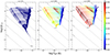 |
Fig. 1. Hertzsprung–Russell diagram of stellar mass models in three sets of initial rotation rates: ωi = 0.00, 0.60, and 0.90 for a given metallicity Z = 0.001, Y = 0.250. The colour bar indicates the evolution of the rotation rate (ω) of each single model. For the sake of clarity, the PMS evolution is cut off in this plot. |
Lowest masses in each set of rotation rates and metallicities (including the sets from Paper I).
As the stars evolve along the MS, the surface angular velocity is increased because of angular momentum transport, and so is the rotation rate. It reaches the highest value around the turn-off region. After the MS, the core contracts and the envelope significantly expands, which significantly decreases the surface angular velocity due to the angular momentum conservation. As low-mass stars evolve further along the RGB and increase their radius, the surface velocity drops rapidly while the angular velocity of the inner core increases (see Cantiello et al. 2014; Nguyen et al. 2022).
During the MS, the intermediate-mass rotating stars become more luminous than their non-rotating counterparts because the core mass increases significantly through rotational mixing. It also increases the core radius and MS lifetime. For example, in the case of Mi = 6 M⊙, the track with ωi = 0.99 has a MS lifetime that is longer by 1.37 times than for its non-rotating counterpart. It simultaneously increases its core mass and radius by approximately 0.22 M⊙ and 0.043 R⊙. This increase is illustrated in Fig. 2 for models with a varying initial mass and ωi. This has consequences for their post-MS phases as well, although their surface velocity evolves similarly to that of low-mass stars. In the He-burning phase (or blue loop), the contraction of their envelope later increases ω.
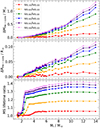 |
Fig. 2. Difference between rotating models and their non-rotating counterparts in He-core mass (top panel), He-core radius (middle panel) at the TAMS (Xc ∼ 10−7), and the MS lifetime ratios (bottom panel). Models from low- to intermediate-mass are shown here with an initial metallicity Z = 0.02. |
3.2. Impact of rotation on surface abundances
In the surface chemical abundances of stars, stellar internal mixing processes can be proved, especially today, when large spectroscopic surveys provide accurate abundances of several elements, for example, the GALactic Archaeology with HERMES (GALAH, Buder et al. 2019), Apache Point Observatory Galactic Evolution Experiment (APOGEE, Abdurro’uf et al. 2022), and Gaia-ESO Gilmore et al. 2022 for hundreds of thousands of stars. Our PARSEC v2.0 evolutionary tracks provide predictions for the surface abundances of several elements (from 1H to 60Zn) along the evolution. Five of these elements are retained in the isochrone tables1, namely 1H, 4He, 12C, 14N, and 16O.
Panels b to j of Fig. 3 show the evolution of several surface abundances and their ratios with respect to the initially assumed values for a few selected elements and stars with and without rotation of initial masses of 1.5 M⊙ and 6 M⊙. In particular, Fig. 3 (b-g, c-h) shows the variation in the C-isotopes and the CN ratios. In standard non-rotating models (cyan lines), the ratios remain the same as their initial values during the MS evolution because there is no active mixing process. The first change in the surface abundances occurs at the beginning of the red giant branch when the downward extension of the convective envelope causes the first dredge-up (1DU). As a consequence, the nuclear burned products 13C and 14N are brought up to the surface, while 12C is depleted (see also Iben 1967; Karakas 2017).
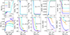 |
Fig. 3. Impact of rotation on the HRD and several surface abundances normalised to their initial values. Models with a mass of 1.5 M⊙ are shown in the top row (panels a-e), and models with a mass of 6 M⊙ are shown in the second row (panels f-j). Different initial rotation rates are shown by different colours. The first column shows the HRD of the selected models. The second and third columns show the C-isotope ratio and the C/N ratio, respectively, with respect to the initial values. That is, we plot the quantity (X/Y)−(X/Y)ini, where X/Y = nX/nY is number density ratio of species X and Y, and the (X/Y)ini value is specified in the plot. The abundances of 16O and 7Li are shown in the fourth and fifth columns, respectively. In the latter cases, we plot the quantity A(X)−A(X)ini, where A(X) = log(nX/nH)+12 is the abundance of element X, and A(X)ini is its initial value, as specified in each panel. nH is the hydrogen density number. The models are shown from the ZAMS to the RGB tip for the 1.5 M⊙ model, and at the end of the He-burning phase for the 6 M⊙. The black dot marks the TAMS. |
When rotation is considered, rotational mixing is established. In the case of intermediate-mass stars where the CNO cycle is the main burning channel (e.g. for the 6 M⊙ star in Fig. 3), a significant decrease in the 12C/13C and 12C/14N ratios from their initial values can be seen during the MS phase. The later evolution shows further depletion mainly due to the 1DU. In general, the decrease is stronger for a higher initial rotational rate. The situation is different in the case of low-mass stars, where the pp-chains are the main burning channels during the MS, and rotational mixing becomes insignificant: Overall, rotation has little impact on the variation in these ratios. This also holds true for the oxygen abundance (Fig. 3d). Instead, rotational mixing in intermediate-mass stars depletes surface oxygen far below the values predicted by the non-rotating 1DU models (Fig. 3i). More extreme rotation rates cause even stronger depletions. This might provide a good explanation for the chemically anomalous stars observed in many open clusters (e.g. Takeda et al. 2018; Lombardo et al. 2021; Casamiquela et al. 2022).
On the other hand, Fig. 3e and j show the variation in surface lithium. A significant amount of lithium can be transferred from the envelope to the inner layers through rotational mixing, where it is eventually destroyed at temperatures of ∼2.6 × 10⁶ K. The efficiency of Li depletion increases with the initial rotation rate, mass, and eventually, the metallicity, as we show below. The need for rotation to explain the observed abundances of lithium in supergiant stars has been suggested variously before (e.g. Lyubimkov et al. 2012; Magrini et al. 2021; Fanelli et al. 2022). The discrepancy between the primordial value (A(Li) = 2.69; Coc et al. 2014) and the Spite plateau (A(Li) = 2.3; Spite & Spite 1982) measured from dwarf-MS low-mass metal-poor stars, which is commonly known as the cosmological lithium problem, requires additional mixing mechanisms in the early evolution up to the terminal-age mains sequence (TAMS) to explain it (see Richard et al. 2005; Fu et al. 2015; Nguyen et al. 2025, for references). We clarify that in the current release, PARSEC v2.0 uses the standard schemes for additional mixing, that is, classical atomic diffusion Bressan et al. 2012 and a fixed value for the efficiency of envelope overshooting. It is therefore reasonable to expect that additional physics needs to be implemented in our models in order to accurately reproduce the Li abundance that is observed in low-mass metal-poor stars.
In Fig. 4 we show the impact of rotation on the CNO abundances of a 6 M⊙ track for different metallicities as a representative of intermediate-mass stars. The bottom panels show the initial abundance of CNO isotopes of our tracks with 13 different metallicities. The upper panels show the difference in the surface CNO abundances between the TAMS and the initial values. The non-rotating models (cyan) show no changes at all metallicities. On the other hand, in the presence of rotational mixing, C and O are depleted and the N abundance is enhanced. More interestingly, Fig. 4 implies that the effect of rotational mixing on the CNO abundances also depends on metallicity, in addition to stellar mass and rotational rate: Its efficiency increases significantly towards lower metallicities because the convective core is more extended.
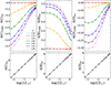 |
Fig. 4. Upper panel: Difference of the surface CNO abundances between the TAMS and initial value for 6 M⊙ stellar tracks with different metallicities and various initial rotation rates. Bottom panel: Initial values of the CNO abundances. The grey star indicates the initial abundances at solar metallicity. |
Similar results are found for the case of lithium, which is shown in the upper panel of Fig. 5, for the 6 M⊙ model. The depletion of lithium caused by rotation ultimately depends on the rotation rate, mass, and metallicity. The middle panel of Fig. 5 also shows the depletion of lithium at log(Z/Z⊙)≥ − 0.6 for the non-rotating 1.5 M⊙ stars. This can be understood by the fact that the convenctive cores of low-mass stars with a higher metallicity are more extended. The temperature at the bottom of the envelopes is already sufficient to destroy lithium during the early evolution. This process is clearly aided by convective envelope overshoot in the models. A dedicated investigation of the lithium evolution in the PMS of low-mass stars will be pursued in a forthcoming work.
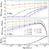 |
Fig. 5. Same as Fig. 4, but for lithium. The upper panel shows the abundance difference for 6 M⊙ stars, the middle panel shows it for 1.5 M⊙ stars, and the bottom panel is the initial 7Li-abundance at a given metallicity. |
3.3. Comparison to GENEC and MIST
The differences between PARSEC v2.0 and its previous version (PARSEC v1.2S) were already extensively discussed in Paper I. In this subsection, we compare our stellar tracks with the GENEC tracks Georgy et al. 2013 and from the MIST database Choi et al. 2016. GENEC computed tracks with the initial rotation rate defined by the tangential velocities, v/vcrit = 0.40, which corresponds to Ω/Ωcrit = 0.59 in terms of angular velocities. Therefore, we computed a few additional tracks (Z = 0.002, M = 4 M⊙) with this initial value of ωi = 0.59 for the sake of comparison. Figure 6 indicates that PARSEC v2.0 tracks are systematically brighter, have less extended blue loops, and have a milder depletion of the oxygen abundance than GENEC tracks.
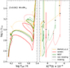 |
Fig. 6. Comparison between the stellar tracks in terms of HRD evolution (left panel) and the surface oxygen mass fraction evolution (right panel). All tracks have an initial metallicity Z = 0.002 and initial mass Mi = 4 M⊙. Non-rotating tracks are shown as solid lines, and rotating tracks are shown as dotted lines. The colour-code indicates the tracks obtained from different databases. Rotating PARSEC v2.0 and GENEC tracks are with ωi = 0.59, and MIST is with ν/νcrit = 0.4. All stellar tracks begin from the ZAMS. The black dots mark the TAMS, and black stars mark the end of the He-burning phase. |
We note that the input physics in the PARSEC v2.0, GENEC, and MIST tracks differ widely. Table 4 presents some of the differences regarding the mixing length parameter, the 12C(α, γ)16O, the 14N(p, γ)15O nuclear reaction rates, and the envelope-overshooting efficiency. In particular, GENEC adopts an overshoot distance of 0.1HP from the Schwarzschild border of the core, while PARSEC v2.0 applies a value of 0.2HP (or, equivalently, a λov = 0.4 across the border; see Bressan et al. 1981). This difference immediately leads to a higher He-core mass in PARSEC v2.0, and thus, to a more luminous track after the MS. This also affects the MS lifetime. For example, the non-rotating 4 M⊙ model shows a difference of 14 Myr between the two codes. Namely, PARSEC v2.0 predicts 138 Myr, and GENEC predicts 124 Myr. We also verified the non-rotating 4 M⊙, Z = 0.002 computed by STAREVOL code Lagarde et al. 2012, with which the MS lifetime of this track is similar to the prediction of GENEC, that is, 126 Myr. Additionally, all the above ingredients directly affect the extent and luminosity of the blue-loop feature of intermediate-mass stars, as shown by Tang et al. 2014.
Input parameters adopted in three stellar evolutionary codes.
We also show in Fig. 6 the interpolated tracks, taken from MIST database, with an initial metallicity Z = 0.002 and mass Mi = 4 M⊙. The HRD evolution of the non-rotating PARSEC v2.0 track is similar to that of MIST. This is mainly because of the equivalent core-overshooting efficiency parameter adopted in PARSEC v2.0 and MIST tracks. Despite the different overshooting implementation (ballistic step for PARSEC v2.0 and exponential decay for MIST), they are about equivalent to a step-overshooting distance of 0.2 HP (see Magic et al. 2010; Choi et al. 2016). They use different criteria, Schwarzschild versus Ledoux, to define the convective regions, which leads to a slight difference in the advanced phases. The MIST track predicts a similar MS lifetime. In particular, the non-rotating 4 M⊙ MIST track gives 137 Myr.
For the comparison of rotating tracks, we selected models with similar initial tangential velocity at the ZAMS. Despite the initial similar configuration, the evolution proceeds differently, not only due to the different non-rotating physical parameters, but also to the different implementation and treatment of angular momentum transport. In particular, GENEC models treat meridional circulation as an advection process and the shear instability as a diffusion process. In PARSEC v2.0, the diffusion scheme is instead used to treat both rotational instabilities. MIST model treats rotation still differently by taking five different rotationally induced instabilities into account Paxton et al. 2013; Choi et al. 2016. These differences directly lead to variations in the distribution of chemical elements along the evolution between different tracks. Regardless of the differences in the initial mass fractions of the adopted chemical mixtures (see Table 4), the impact of rotational mixing can be seen by the amount of surface oxygen that is depleted throughout the evolution. For example, in the case shown here, the TAMS of the PARSEC v2.0 track decreases modestly ΔXO ≈ 1 × 10⁻⁵ from its initial value. On the other hand, GENEC tracks deplete it more strongly, ΔXO ≈ 9 × 10⁻⁵, which can only be due to the different efficiencies of rotational mixing. Similar to GENEC, the rotating MIST track with ν/νcrit = 0.4 shows ΔXO ≈ 7 × 10⁻⁵.
After the TAMS, when the stars begin 1DU, together with the effect of rotational mixing, the rotating tracks show a significant depletion of surface oxygen. This is seen in all PARSEC v2.0, GENEC, and MIST rotating tracks. The same trends are seen for the depletion of 12C and the enhancement of 14N.
4. Isochrones
In Paper I, isochrones were derived for the same seven values of ωi at which evolutionary tracks were computed. This involved interpolating in the plane of initial mass and age defined by every grid of evolutionary tracks of a given ωi. Interpolation between tracks of different metallicities was also allowed.
Since then, we improved the interpolation algorithms of the TRIdimensional modeL of thE GALaxy code (TRILEGAL, Girardi et al. 2005; Marigo et al. 2017) so as to also allow for the interpolation between grids with different ωi. The interpolation method is essentially the same as was described by Bertelli et al. 2008 to produce isochrones at different values of metallicity and helium content. This means that isochrones can now be produced for any ωi value in the interval from 0.00 to 0.99. This new interpolation scheme is now available at the CMD v3.8 web interface2.
To test this new interpolation algorithm, we produced a number of isochrones of a given ωi = 0.90 and Z = 0.006 that were computed 1) with the actual set of computed tracks, and 2) by the interpolation between two neighbouring values of ωi = 0.80 and 0.95. Figure 7 shows the produced isochrones by the two methods for ages log t/yr = 8.0 − 9.5. The isochrones produced by the interpolation algorithm are very similar to those produced directly from the ωi = 0.90 tracks. Small differences can be found just in the turn-off region, with the level of ΔTeff = 0.006 dex (upper right panel), and at the transition mass at which rotation is assumed to start being efficient (bottom right panel). It is expected that the typical errors caused by the interpolation in ωi are smaller than these indicative examples.
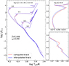 |
Fig. 7. Comparison of theoretical isochrones produced by the computed stellar tracks (red) and the interpolation algorithm (blue). The isochrones are for an initial metallicity of Z = 0.006, ωi = 0.90, and the ages are indicated in the plot. The right panels are zoomed in to the turn-off region (upper panel) and the lower-MS part (bottom panel) of the isochrones of log t/yr = 8.5. |
With the new tracks, we computed the corresponding isochrones, from which we also derived the absolute magnitudes by applying the bolometric corrections (BCs) by Girardi et al. 2019. These BCs were suitably computed for rotating stars as a function of the stellar inclination i. They were made available for the passbands of many different photometric systems (see Chen et al. 2019).
We note that the inclination-dependent BCs described by Girardi et al. 2019 cannot be computed for the coolest stars because current libraries of model atmospheres are limited. This is less of a problem in our case because ω of initially fast-rotating stars is reduced to values of ∼0.1 when the stars reach a mean effective temperature cooler than ∼5000 K. These stars deviate very little from spherical symmetry, and they can be described by a single Teff value. Therefore, for Teff < 5130 K, we adopted the BCs derived from non-rotating models (i.e. derived from plane-parallel model atmospheres, as in Girardi et al. 2002). In the interval from 5370 to 5130 K, we smoothly interpolated between the BCs derived from rotating stars and those derived from non-rotating stars.
Finally, a brief explanation of the quantities presented in the isochrone tables can be found in a dedicated document3. For the quantities presented in the track tables, we refer to anther dedicated document4.
5. Comparison with observations
In order to verify the quality of our models, we compared them with observations of the young cluster NGC 6067. The age of this cluster was estimated between 50 and 150 Myr Thackeray et al. 1962; Santos & Bica 1993; Majaess et al. 2013, and the metallicity varies from solar to supersolar value. For instance, Piatti et al. 1995 derived a mean metallicity of [Fe/H]= − 0.01 ± 0.07 dex, while Alonso-Santiago et al. 2017 suggested a mean value of 0.19 ± 0.05 dex. The metallicity of the renowned Cepheid V340 Nor in this cluster is estimated to be a near-solar value, for which different works agree well (e.g. Alonso-Santiago et al. 2017 claimed [Fe/H] = 0.09 ± 0.11 dex, and Genovali et al. 2014 claimed [Fe/H] = 0.07 ± 0.1 dex). The reddening and distance modulus of NGC 6067 are also well constrained in the literature. Recent studies reported a reddening E(B − V)≈0.34 ± 0.04 mag (e.g. An et al. 2007; Jackson et al. 2020, 2022). For the true distance modulus, Cantat-Gaudin et al. 2020 reported a value of (m − M)0 = 11.37 ± 0.2 mag, while Peña Ramírez et al. 2021 claimed a value of 11.74 ± 0.26 mag, and Jackson et al. 2022 provided an intermediate value of 11.62 ± 0.15 mag. Within the uncertainties, they tend to agree with each other.
Moreover, the recent Gaia DR3 data contain the broadening velocity (vbroad) derived with the Radial Velocity Spectrometer (RVS) for more than three million bright (G < 12 mag) targets Gaia Collaboration 2023. This broadening velocity includes the contributions of the projected rotational velocity and the macroturbulent velocity, as well as other effects. For rotating stars, vbroad was shown to be an excellent proxy for the projected rotational velocity, v sin i (see also Cordoni et al. 2024).
We compared the observed vbroad with the tangential velocity predicted in our models (see also Cordoni et al. 2024). Before we start, we note that the tangential velocity should be compared with the upper values of vbroad because the observed velocity is reduced by the (unknown) projection factor sin i.
Figure 8 shows the variation in vbroad versus the Gaia colour of stars in the cluster NGC 6067. The data were retrieved from the Gaia DR3 archive5 Frémat et al. 2023. In total, we found that only 53 stars from the NGC 6067 sample have available vbroad values because the catalogue is currently limited to GRVS < 12 mag. By selecting stars with a high membership probability of only (proba ≥ 0.89), we reduced the sample to 25 stars. Among these, stars at the MS turn-off show a wide range of vbroad values spanning from a few dozen km/s up to the extremely fast at ∼400 km/s. On the other hand, cool stars on the red side have significantly lower vbroad values (lower than ∼20 km/s), as expected from the significant expansion of their envelopes, which rapidly decreases the surface rotational velocity. We clarify that the Gaia vbroad < 10 km/s is unreliable because the measurements were limited (see Frémat et al. 2023). Nonetheless, the cepheid V340 Nor, which is very well studied and was used as a benchmark for many calibrations, is presented in the sample with vbroad ∼ 17.4 ± 9.3 km/s. In order to determine the location of V340 Nor in the plot, we cross-matched its (RA, Dec) from the sample of Alonso-Santiago et al. 2017 with the Gaia catalogue.
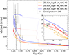 |
Fig. 8. Broadening velocity of 25 star members of NGC 6067. The surface tangential velocity from the isochrone models is shown with an inclination angle i = 90o (i = 0o stars have a similar range in colour and negligible vbroad). The solid line represents the upper MS evolution and after (Gmag < 14 mag). The dotted lines represent the lower MS part of the isochrones (Gmag > 14 mag). The inset panel zooms into the cool-stars region. |
In Fig. 8 we plot the tangential velocities predicted from our models are plotted as solid lines. Our extremely fast rotating model with ωi ≈ 0.95 reproduces the extremely high vbroad in the turn-off region very well. Stars with a milder vbroad at the turn-off are either stars with similar ωi observed at small inclination, or stars with ωi ≃ 0.64 observed at high inclination. The same ωi ≃ 0.64 values suffice to explain the vbroad of the cool stars, including 340_Nor, although models with higher ωi and a low inclination cannot be excluded. On the other hand, a significant group of four cool stars could be explained with a lower rotation rate, namely ωi = 0.43, implying that they might be observed at high inclination.
The CMD fit in the Gaia passbands is shown in Fig. 9 with the adopted data from Cantat-Gaudin & Anders 2020, where only members with the probability ≥0.89 are selected, together with the 25 stars whose published vbroad are shown as green triangles. The results of Alonso-Santiago et al. 2017 indicated a spread in metallicity within the observed stars in their sample. In particular, 4 of the 13 cool stars have [Fe/H] ≤ 0.1 dex, including the cepheid V340 Nor. The other stars have a mean value of about [Fe/H] ≈ 0.2 dex. By using the Padova isochrones Girardi et al. 2000 where rotation was not yet implemented, Alonso-Santiago et al. 2017 found no conclusive evidence of multiple populations in this cluster. In this work, we revisited the CMD of NGC 6067 with our rotating models and explored the multiple populations in this cluster.
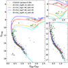 |
Fig. 9. CMD of NGC 6067. The data were adopted from the Gaia DR2 catalogue Cantat-Gaudin & Anders 2020, and stars with a membership probability ≥0.89 are shown. Stars with vbroad are shown as green triangles. The isochrones with the adopted metallicity (Z = 0.016), ages (log t/yr = 7.86 and 8.14), and initial rotational rates (ωi = 0.43, 0.64 and 0.95) are plotted as solid (i = 0°) and dotted lines (i = 90°). |
For this purpose, an intermediate true distance modulus of (m − M)0 = 11.50 mag was adopted from the literature (see Cantat-Gaudin et al. 2020; Peña Ramírez et al. 2021; Jackson et al. 2022). The extinction AV = 1.10 mag was selected so as to fit the position of MS stars (Gmag > 10). Although the metallicity spread found by Alonso-Santiago et al. 2017 is still debated, we chose a metallicity slightly above the solar value for our isochrones (Z = 0.016) and investigated whether a higher metallicity is needed. Our isochrone with an age of log(t/yr) = 8.14 (∼138 Myr), and ωi = 0.43 fits the cool stars best (with Gmag > 9), which are assumed to be in the core He-burning phase, and with the MS part of the cluster. For the most luminous stars (Cepheid V340 Nor and the K2 type 261 star), our isochrone with the same metallicity but with a younger age, log t = 7.86 (∼72 Myr) and higher ωi = 0.64 fits the data well. As mentioned above (Fig. 8), the choice of these rotating models explains the observed vbroad of these cool stars well. Models with extremely high rotation or non-rotating models, on the other hand, fail to reproduce the CMD of this cluster. In particular, the ωi = 0.95 model with log(t/yr) = 7.86 is too bright to reproduce the location of the luminous stars. Similarly, with the same choice of parameters, the non-rotating model fails to reproduce the He-burning stars.
As a result, the Gaia CMD fits show that no higher metallicity is required for NGC 6067. To further confirm the fits above, we performed the CMD fit based on the VISTA photometry system, as shown in Fig. 10. The upper panel shows the observed CMD for a total of 42 stars from Alonso-Santiago et al. 2017 (green dots), together with the sample of Peña Ramírez et al. 2021 in the background (grey dots). The best-fit models from Fig. 9 were adopted in this plot. The isochrones in the VISTA CMD agree well with our findings with the Gaia passbands.
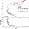 |
Fig. 10. Top panel: CMD of NGC 6067 in Vista photometry. The green dots are data adopted from Alonso-Santiago et al. 2017, and the grey dots are data adopted from Peña Ramírez et al. 2021. The superimposed isochrones are models with the same parameters as in Figs. 8 and 9. Bottom panel: Rotational velocity of stars from the Alonso-Santiago et al. 2017 catalogue, superimposed with the predictions from isochrone models (solid lines show the evolution with KS < 13 mag, and dotted lines show KS > 13 mag). Only stars with precise v sin i and ξ are presented in this plot. |
The location of the cepheid QZ Nor in Fig. 10 is not reproduced very well by the isochrones. Nonetheless, it is unclear whether QZ Nor is a member of NGC 6067 (see Peña Ramírez et al. 2021), and we thus chose not to rely on QZ Nor for our discussion of the model fits above.
The bottom panel of Fig. 10 shows the sum of the projected rotational velocity (v sin i) and the macroturbulent velocity (ξ) of the stars in the sample of Alonso-Santiago et al. 2017. We only selected non-binary stars with precise measured values in both velocities for the plot. The sum velocity of cepheid V340 Nor is 13 ± 5.6 km/s. Our rotating models fit its velocity very well. Most stars in the MS turn-off are reproduced by our best-fit models, with a velocity below 200 km/s. The B-type star with an emission line (Be-star) 294 is an exception. It has v sin i = 279.6 ± 9.1 km/s and ξ = 23.7 ± 19.4 km/s, which are well reproduced by our extremely fast-rotating models (ωi = 0.95) in general. Figs. 8 and 9 show, however, that this model fails to reproduce the observed CMD of the cluster in the Gaia and VISTA filters.
Similarly, Meilland et al. 2012 also found that Be-stars are extremely fast-rotating stars. They are surrounded by a gaseous circumstellar environment that might be the origin of their fast-rotating behaviour (see also Rivinius et al. 2006). Moreover, Granada et al. 2013 suggested a mass and/or Teff dependence on the rotational rate in order to explain the Be star phenomenon. A detailed model for the Be star phenomenon is beyond the scope of this paper, however.
Furthermore, Alonso-Santiago et al. 2017 reported the surface abundances of many cool stars in their sample. We paid particular attention to the oxygen abundance of these stars because our isochrone tables include the variation of three isotopes, 12C, 14N, and 16O. Figure 11 showed their observed [O/H] values, together with the prediction from our best-fit models. First of all, the measured [O/H] are clearly spread: Six stars have nearly solar values, but five stars are strongly depleted in oxygen. The isochrones with different ages indicate a very modest change in [O/H], while rotation enhances the depletion of the O abundance, as expected. Our best-fit ωi = 0.64 model is not enough to explain the four stars that are significantly depleted, however, even with their 1σ uncertainty. The model with a lower metallicity might be able to explain the strongly [O/H] depleted stars. The rotating GENEC model Ekström et al. 2012 with Z = 0.014 provides a similar prediction. The prediction from both models suggests that a lower metallicity is required in order to reproduce the significant depletion [O/H]. On the other hand, the result from the CMD fits above shows no clear evidence of a metallicity spread in this cluster. We also recall, however, that the data show large error bars. This makes it difficult to reach any firm conclusion on the properties of the cluster stars. A more thorough selection of their chemical abundances together with a more detailed analysis are required. We will address this in forthcoming works.
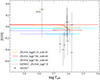 |
Fig. 11. Oxygen-hydrogen ratio of cool stars by Alonso-Santiago et al. 2017. The prediction from best-fit models is shown as solid lines. The prediction from the GENEC model (Z = 0.014, log t = 7.8, ωi = 0.59) is plotted for comparison. |
The discussion above illustrates the general difficulties of simultaneously interpreting current data for open clusters on photometry, projected velocities, and abundance variations. It also show that large sets of isochrones which include the effect of rotation are clearly needed in the era of Gaia data and of large spectroscopic surveys.
6. Summary and conclusion
We presented the new calculation of stellar evolutionary tracks and isochrones for seven metallicities to complement the first release of PARSEC v2.0 in Paper I. In total, we covered the metallicity range from Z = 0.0001 to 0.03. In order to be homogeneously consistent with the first release, we adopted the same input physics as Paper I for our calculations. We covered the mass range from ∼0.7 − 14 M⊙, with seven initial rotation rates spanning from ωi = 0.00 to 0.99 that depended on the initial masses. The details of the input physics are described in Sect. 2, and the impact of rotation on the stellar structure and evolution is studied in Sect. 3.
In this second release, we include the surface abundances of several more isotopes (from 1H to 60Zn) in the stellar track table. We simultaneously present five of them (1H, 4He, 12C, 14N, 16O) in the isochrone table, with the possibility of adding more isotopes upon request. We also upgrade the isochrone web-interface, in which the isochrones with an intermediate rotation rate between the computed values can now be archived by an interpolation scheme that is described in Sect. 4.
We verified the quality of our new computed models by comparisons with the observed data of the open cluster NGC 6067 in terms of broadening velocity, photometric colour-magnitude diagram, and oxygen abundances. The results indicate that rotating models are crucial for explaining the extremely fast-rotating stars in the turn-off region of the cluster. On the other hand, our rotating models suggest that at least two populations are harboured in the cluster, with a dispersion in age and initial rotation rate. The populations have the same metallicity. In contrast, the observed oxygen abundance of cool-star members requires a lower metallicity. The large uncertainty from the observed [O/H] prevented us from finding conclusive evidence in this regard.
Finally, to reiterate, all the stellar evolutionary tracks we discussed, including the previous database presented in Paper I, are available at a dedicated website6. The corresponding isochrones with the new interpolation in the initial rotational rate can be obtained at another dedicated website7.
We recall that surface abundances of other elements and isotopes (e.g., 18O, 13C, 7Li, etc.) can be added to the isochrones as well, upon reasonable request to the main authors.
Acknowledgments
We thank the referee (Devesh Nandal) for the thorough and constructive comments/suggestions. This project has received funding from the European Union’s Horizon 2020 research and innovation programme under grant agreement No 101008324 (ChETEC-INFRA). We also acknowledge the financial support from INAF Theory Grant 2022. We acknowledge the Italian Ministerial grant PRIN2022, “Radiative opacities for astrophysical applications”, no. 2022NEXMP8. GC acknowledges partial financial support from European Union–Next Generation EU, Mission 4, Component 2, CUP: C93C24004920006, project ‘FIRES’. The contribution by MT and GP is funded by the European Union – NextGenerationEU and by the University of Padua under the 2023 STARS Grants@Unipd programme (“CONVERGENCE: CONstraining the Variability of Evolved Red Giants for ENhancing the Comprehension of Exoplanets”). CTN acknowledges the support by INAF Mini grant 2024, “GALoMS – Galactic Archaeology for Low Mass Stars”. AJK acknowledges support by the Swedish National Space Agency (SNSA). GE acknowledges the contribution of the Next Generation EU funds within the National Recovery and Resilience Plan (PNRR), Mission 4 – Education and Research, Component 2 – From Research to Business (M4C2), Investment Line 3.1 – Strengthening and creation of Research Infrastructures, Project IR0000034 – “STILES - Strengthening the Italian Leadership in ELT and SKA”. YC acknowledges the Natural Science Research Project of Anhui Educational Committee No. 2024AH050049, National Natural Science Foundation of China (NSFC) No. 12003001, the Anhui Project (Z010118169)
References
- Abdurro’uf, Accetta, K., Aerts, C., et al. 2022, ApJS, 259, 35 [NASA ADS] [CrossRef] [Google Scholar]
- Alongi, M., Bertelli, G., Bressan, A., & Chiosi, C. 1991, A&A, 244, 95 [NASA ADS] [Google Scholar]
- Alonso-Santiago, J., Negueruela, I., Marco, A., et al. 2017, MNRAS, 469, 1330 [NASA ADS] [CrossRef] [Google Scholar]
- Amard, L., Palacios, A., Charbonnel, C., et al. 2019, A&A, 631, A77 [NASA ADS] [CrossRef] [EDP Sciences] [Google Scholar]
- An, D., Terndrup, D. M., & Pinsonneault, M. H. 2007, ApJ, 671, 1640 [Google Scholar]
- Asplund, M., Grevesse, N., & Sauval, A. J. 2005, in Cosmic Abundances as Records of Stellar Evolution and Nucleosynthesis, eds. I. Barnes, G. Thomas, & F. N. Bash, ASP Conf. Ser., 336, 25 [NASA ADS] [Google Scholar]
- Asplund, M., Grevesse, N., Sauval, A. J., & Scott, P. 2009, ARA&A, 47, 481 [NASA ADS] [CrossRef] [Google Scholar]
- Bastian, N., & de Mink, S. E. 2009, MNRAS, 398, L11 [NASA ADS] [CrossRef] [Google Scholar]
- Bertelli, G., Girardi, L., Marigo, P., & Nasi, E. 2008, A&A, 484, 815 [NASA ADS] [CrossRef] [EDP Sciences] [Google Scholar]
- Bjorkman, J. E., & Cassinelli, J. P. 1993, ApJ, 409, 429 [NASA ADS] [CrossRef] [Google Scholar]
- Böhm, K. H. 1958, ZAp, 46, 245 [Google Scholar]
- Borisov, S., Charbonnel, C., Prantzos, N., Dumont, T., & Palacios, A. 2024, A&A, 690, A245 [NASA ADS] [CrossRef] [EDP Sciences] [Google Scholar]
- Brandt, T. D., & Huang, C. X. 2015, ApJ, 807, 25 [NASA ADS] [CrossRef] [Google Scholar]
- Bressan, A. G., Chiosi, C., & Bertelli, G. 1981, A&A, 102, 25 [Google Scholar]
- Bressan, A., Marigo, P., Girardi, L., et al. 2012, MNRAS, 427, 127 [NASA ADS] [CrossRef] [Google Scholar]
- Brott, I., de Mink, S. E., Cantiello, M., et al. 2011, A&A, 530, A115 [NASA ADS] [CrossRef] [EDP Sciences] [Google Scholar]
- Buchmann, L. 1997, ApJ, 479, L153 [Google Scholar]
- Buder, S., Lind, K., Ness, M. K., et al. 2019, A&A, 624, A19 [NASA ADS] [CrossRef] [EDP Sciences] [Google Scholar]
- Caffau, E., Ludwig, H. G., Steffen, M., Freytag, B., & Bonifacio, P. 2011, Sol. Phys., 268, 255 [Google Scholar]
- Cantat-Gaudin, T., & Anders, F. 2020, A&A, 633, A99 [NASA ADS] [CrossRef] [EDP Sciences] [Google Scholar]
- Cantat-Gaudin, T., Anders, F., Castro-Ginard, A., et al. 2020, A&A, 640, A1 [NASA ADS] [CrossRef] [EDP Sciences] [Google Scholar]
- Cantiello, M., Mankovich, C., Bildsten, L., Christensen-Dalsgaard, J., & Paxton, B. 2014, ApJ, 788, 93 [Google Scholar]
- Casamiquela, L., Gebran, M., Agüeros, M. A., Bouy, H., & Soubiran, C. 2022, AJ, 164, 255 [NASA ADS] [CrossRef] [Google Scholar]
- Chen, Y., Girardi, L., Bressan, A., et al. 2014, MNRAS, 444, 2525 [Google Scholar]
- Chen, Y., Girardi, L., Fu, X., et al. 2019, A&A, 632, A105 [EDP Sciences] [Google Scholar]
- Chieffi, A., & Limongi, M. 2013, ApJ, 764, 21 [Google Scholar]
- Choi, J., Dotter, A., Conroy, C., et al. 2016, ApJ, 823, 102 [Google Scholar]
- Claret, A., & Torres, G. 2016, A&A, 592, A15 [NASA ADS] [CrossRef] [EDP Sciences] [Google Scholar]
- Claret, A., & Torres, G. 2017, ApJ, 849, 18 [Google Scholar]
- Claret, A., & Torres, G. 2018, ApJ, 859, 100 [Google Scholar]
- Claret, A., & Torres, G. 2019, ApJ, 876, 134 [Google Scholar]
- Coc, A., Goriely, S., Xu, Y., Saimpert, M., & Vangioni, E. 2012, ApJ, 744, 158 [NASA ADS] [CrossRef] [Google Scholar]
- Coc, A., Uzan, J.-P., & Vangioni, E. 2014, JCAP, 2014, 050 [Google Scholar]
- Cordoni, G., Milone, A. P., Marino, A. F., et al. 2018, ApJ, 869, 139 [CrossRef] [Google Scholar]
- Cordoni, G., Casagrande, L., Yu, J., et al. 2024, MNRAS, 532, 1547 [CrossRef] [Google Scholar]
- Costa, G., Girardi, L., Bressan, A., et al. 2019a, A&A, 631, A128 [NASA ADS] [CrossRef] [EDP Sciences] [Google Scholar]
- Costa, G., Girardi, L., Bressan, A., et al. 2019b, MNRAS, 485, 4641 [NASA ADS] [CrossRef] [Google Scholar]
- Costa, G., Bressan, A., Mapelli, M., et al. 2021, MNRAS, 501, 4514 [NASA ADS] [CrossRef] [Google Scholar]
- Costa, G., Shepherd, K. G., Bressan, A., et al. 2025, A&A, 694, A193 [NASA ADS] [CrossRef] [EDP Sciences] [Google Scholar]
- Cyburt, R. H., Hoffman, R., & Woosley, S. 2012, https://reaclib.jinaweb.org/labels.php?action=viewLabellabel=chw0 [Google Scholar]
- de Jager, C., Nieuwenhuijzen, H., & van der Hucht, K. A. 1988, A&AS, 72, 259 [NASA ADS] [Google Scholar]
- Ekström, S., Georgy, C., Eggenberger, P., et al. 2012, A&A, 537, A146 [Google Scholar]
- Ettorre, G., Mazzi, A., Girardi, L., et al. 2025, MNRAS, 539, 2537 [Google Scholar]
- Fanelli, C., Origlia, L., Mucciarelli, A., et al. 2022, ApJ, 931, 61 [Google Scholar]
- Frémat, Y., Royer, F., Marchal, O., et al. 2023, A&A, 674, A8 [NASA ADS] [CrossRef] [EDP Sciences] [Google Scholar]
- Friend, D. B., & Abbott, D. C. 1986, ApJ, 311, 701 [Google Scholar]
- Fu, X., Bressan, A., Molaro, P., & Marigo, P. 2015, MNRAS, 452, 3256 [CrossRef] [Google Scholar]
- Fu, X., Bressan, A., Marigo, P., et al. 2018, MNRAS, 476, 496 [NASA ADS] [CrossRef] [Google Scholar]
- Gaia Collaboration (Vallenari, A., et al.) 2023, A&A, 674, A1 [NASA ADS] [CrossRef] [EDP Sciences] [Google Scholar]
- Genovali, K., Lemasle, B., Bono, G., et al. 2014, A&A, 566, A37 [NASA ADS] [CrossRef] [EDP Sciences] [Google Scholar]
- Georgy, C., Ekström, S., Meynet, G., et al. 2012, A&A, 542, A29 [NASA ADS] [CrossRef] [EDP Sciences] [Google Scholar]
- Georgy, C., Ekström, S., Eggenberger, P., et al. 2013, A&A, 558, A103 [NASA ADS] [CrossRef] [EDP Sciences] [Google Scholar]
- Gilmore, G., Randich, S., Worley, C. C., et al. 2022, A&A, 666, A120 [NASA ADS] [CrossRef] [EDP Sciences] [Google Scholar]
- Girardi, L., Bressan, A., Bertelli, G., & Chiosi, C. 2000, A&AS, 141, 371 [NASA ADS] [CrossRef] [EDP Sciences] [Google Scholar]
- Girardi, L., Bertelli, G., Bressan, A., et al. 2002, A&A, 391, 195 [NASA ADS] [CrossRef] [EDP Sciences] [Google Scholar]
- Girardi, L., Groenewegen, M. A. T., Hatziminaoglou, E., & da Costa, L. 2005, A&A, 436, 895 [NASA ADS] [CrossRef] [EDP Sciences] [Google Scholar]
- Girardi, L., Costa, G., Chen, Y., et al. 2019, MNRAS, 488, 696 [CrossRef] [Google Scholar]
- Granada, A., Ekström, S., Georgy, C., et al. 2013, A&A, 553, A25 [NASA ADS] [CrossRef] [EDP Sciences] [Google Scholar]
- Groh, J. H., Ekström, S., Georgy, C., et al. 2019, A&A, 627, A24 [NASA ADS] [CrossRef] [EDP Sciences] [Google Scholar]
- Hastings, B., Langer, N., & Puls, J. 2023, A&A, 672, A60 [NASA ADS] [CrossRef] [EDP Sciences] [Google Scholar]
- He, C., Sun, W., Li, C., et al. 2022, ApJ, 938, 42 [Google Scholar]
- Iben, I., Jr 1967, ARA&A, 5, 571 [NASA ADS] [CrossRef] [Google Scholar]
- Imbriani, G., Costantini, H., Formicola, A., et al. 2005, Eur. Phys. J. A, 25, 455 [Google Scholar]
- Jackson, R. J., Jeffries, R. D., Wright, N. J., et al. 2020, MNRAS, 496, 4701 [NASA ADS] [CrossRef] [Google Scholar]
- Jackson, R. J., Jeffries, R. D., Wright, N. J., et al. 2022, MNRAS, 509, 1664 [Google Scholar]
- Karakas, A. I. 2017, in Handbook of Supernovae, eds. A. W. Alsabti, & P. Murdin, 461 [Google Scholar]
- Komatsu, E., Smith, K. M., Dunkley, J., et al. 2011, ApJS, 192, 18 [Google Scholar]
- Kunz, R., Fey, M., Jaeger, M., et al. 2002, ApJ, 567, 643 [CrossRef] [Google Scholar]
- Lagarde, N., Decressin, T., Charbonnel, C., et al. 2012, A&A, 543, A108 [NASA ADS] [CrossRef] [EDP Sciences] [Google Scholar]
- Limongi, M., & Chieffi, A. 2018, ApJS, 237, 13 [NASA ADS] [CrossRef] [Google Scholar]
- Lombardo, L., François, P., Bonifacio, P., et al. 2021, A&A, 656, A155 [NASA ADS] [CrossRef] [EDP Sciences] [Google Scholar]
- Lyubimkov, L. S., Lambert, D. L., Kaminsky, B. M., et al. 2012, MNRAS, 427, 11 [Google Scholar]
- Maeder, A. 2009, Physics, Formation and Evolution of Rotating Stars (Berlin Heidelberg: Springer) [Google Scholar]
- Magic, Z., Serenelli, A., Weiss, A., & Chaboyer, B. 2010, ApJ, 718, 1378 [NASA ADS] [CrossRef] [Google Scholar]
- Magrini, L., Lagarde, N., Charbonnel, C., et al. 2021, A&A, 651, A84 [NASA ADS] [CrossRef] [EDP Sciences] [Google Scholar]
- Majaess, D., Sturch, L., Moni Bidin, C., et al. 2013, Ap&SS, 347, 61 [NASA ADS] [CrossRef] [Google Scholar]
- Marigo, P., Girardi, L., Bressan, A., et al. 2017, ApJ, 835, 77 [Google Scholar]
- McQuillan, A., Mazeh, T., & Aigrain, S. 2014, ApJS, 211, 24 [Google Scholar]
- Meilland, A., Millour, F., Kanaan, S., et al. 2012, A&A, 538, A110 [CrossRef] [EDP Sciences] [Google Scholar]
- Meynet, G., & Maeder, A. 2000, A&A, 361, 101 [NASA ADS] [Google Scholar]
- Miglio, A., Brogaard, K., Stello, D., et al. 2012, MNRAS, 419, 2077 [Google Scholar]
- Milone, A. P., Marino, A. F., D’Antona, F., et al. 2017, MNRAS, 465, 4363 [NASA ADS] [CrossRef] [Google Scholar]
- Milone, A. P., Marino, A. F., Di Criscienzo, M., et al. 2018, MNRAS, 477, 2640 [Google Scholar]
- Mukhamedzhanov, A. M., Bém, P., Burjan, V., et al. 2008, Phys. Rev. C, 78, 015804 [Google Scholar]
- Nguyen, C. T., Costa, G., Girardi, L., et al. 2022, A&A, 665, A126 [NASA ADS] [CrossRef] [EDP Sciences] [Google Scholar]
- Nguyen, C. T., Bressan, A., Korn, A. J., et al. 2025, A&A, 696, A136 [NASA ADS] [CrossRef] [EDP Sciences] [Google Scholar]
- Paxton, B., Cantiello, M., Arras, P., et al. 2013, ApJS, 208, 4 [Google Scholar]
- Paxton, B., Smolec, R., Schwab, J., et al. 2019, ApJS, 243, 10 [Google Scholar]
- Peña Ramírez, K., González-Fernández, C., Chené, A. N., & Ramírez Alegría, S. 2021, MNRAS, 503, 1864 [CrossRef] [Google Scholar]
- Piatti, A. E., Claria, J. J., & Abadi, M. G. 1995, AJ, 110, 2813 [NASA ADS] [CrossRef] [Google Scholar]
- Reimers, D. 1975, Memoires of the Societe Royale des Sciences de Liege, 8, 369 [Google Scholar]
- Reimers, D. 1977, A&A, 61, 217 [NASA ADS] [Google Scholar]
- Richard, O., Michaud, G., & Richer, J. 2005, ApJ, 619, 538 [Google Scholar]
- Rivinius, T., Štefl, S., & Baade, D. 2006, A&A, 459, 137 [NASA ADS] [CrossRef] [EDP Sciences] [Google Scholar]
- Santos, J. F. C., Jr, & Bica, E. 1993, MNRAS, 260, 915 [Google Scholar]
- Sibony, Y., Shepherd, K. G., Yusof, N., et al. 2024, A&A, 690, A91 [NASA ADS] [CrossRef] [EDP Sciences] [Google Scholar]
- Spite, F., & Spite, M. 1982, A&A, 115, 357 [NASA ADS] [Google Scholar]
- Takeda, Y., Kawanomoto, S., Ohishi, N., et al. 2018, PASJ, 70, 91 [NASA ADS] [Google Scholar]
- Tang, J., Bressan, A., Rosenfield, P., et al. 2014, MNRAS, 445, 4287 [NASA ADS] [CrossRef] [Google Scholar]
- Thackeray, A. D., Wesselink, A. J., & Harding, G. A. 1962, MNRAS, 124, 445 [Google Scholar]
- Vink, J. S., de Koter, A., & Lamers, H. J. G. L. M. 2001, A&A, 369, 574 [NASA ADS] [CrossRef] [EDP Sciences] [Google Scholar]
- von Zeipel, H. 1924, MNRAS, 84, 684 [NASA ADS] [CrossRef] [Google Scholar]
- Yang, W., Bi, S., Meng, X., & Liu, Z. 2013, ApJ, 776, 112 [NASA ADS] [CrossRef] [Google Scholar]
- Yusof, N., Hirschi, R., Eggenberger, P., et al. 2022, MNRAS, 511, 2814 [NASA ADS] [CrossRef] [Google Scholar]
All Tables
Initial masses at the transition between distinct overshooting prescriptions as a function of initial metallicity.
Initial mass value at the transition from low- to intermediate-mass stars as a function of the initial metallicity and rotation rate.
Lowest masses in each set of rotation rates and metallicities (including the sets from Paper I).
All Figures
|
Fig. 1. Hertzsprung–Russell diagram of stellar mass models in three sets of initial rotation rates: ωi = 0.00, 0.60, and 0.90 for a given metallicity Z = 0.001, Y = 0.250. The colour bar indicates the evolution of the rotation rate (ω) of each single model. For the sake of clarity, the PMS evolution is cut off in this plot. |
| In the text | |
|
Fig. 2. Difference between rotating models and their non-rotating counterparts in He-core mass (top panel), He-core radius (middle panel) at the TAMS (Xc ∼ 10−7), and the MS lifetime ratios (bottom panel). Models from low- to intermediate-mass are shown here with an initial metallicity Z = 0.02. |
| In the text | |
|
Fig. 3. Impact of rotation on the HRD and several surface abundances normalised to their initial values. Models with a mass of 1.5 M⊙ are shown in the top row (panels a-e), and models with a mass of 6 M⊙ are shown in the second row (panels f-j). Different initial rotation rates are shown by different colours. The first column shows the HRD of the selected models. The second and third columns show the C-isotope ratio and the C/N ratio, respectively, with respect to the initial values. That is, we plot the quantity (X/Y)−(X/Y)ini, where X/Y = nX/nY is number density ratio of species X and Y, and the (X/Y)ini value is specified in the plot. The abundances of 16O and 7Li are shown in the fourth and fifth columns, respectively. In the latter cases, we plot the quantity A(X)−A(X)ini, where A(X) = log(nX/nH)+12 is the abundance of element X, and A(X)ini is its initial value, as specified in each panel. nH is the hydrogen density number. The models are shown from the ZAMS to the RGB tip for the 1.5 M⊙ model, and at the end of the He-burning phase for the 6 M⊙. The black dot marks the TAMS. |
| In the text | |
|
Fig. 4. Upper panel: Difference of the surface CNO abundances between the TAMS and initial value for 6 M⊙ stellar tracks with different metallicities and various initial rotation rates. Bottom panel: Initial values of the CNO abundances. The grey star indicates the initial abundances at solar metallicity. |
| In the text | |
|
Fig. 5. Same as Fig. 4, but for lithium. The upper panel shows the abundance difference for 6 M⊙ stars, the middle panel shows it for 1.5 M⊙ stars, and the bottom panel is the initial 7Li-abundance at a given metallicity. |
| In the text | |
|
Fig. 6. Comparison between the stellar tracks in terms of HRD evolution (left panel) and the surface oxygen mass fraction evolution (right panel). All tracks have an initial metallicity Z = 0.002 and initial mass Mi = 4 M⊙. Non-rotating tracks are shown as solid lines, and rotating tracks are shown as dotted lines. The colour-code indicates the tracks obtained from different databases. Rotating PARSEC v2.0 and GENEC tracks are with ωi = 0.59, and MIST is with ν/νcrit = 0.4. All stellar tracks begin from the ZAMS. The black dots mark the TAMS, and black stars mark the end of the He-burning phase. |
| In the text | |
|
Fig. 7. Comparison of theoretical isochrones produced by the computed stellar tracks (red) and the interpolation algorithm (blue). The isochrones are for an initial metallicity of Z = 0.006, ωi = 0.90, and the ages are indicated in the plot. The right panels are zoomed in to the turn-off region (upper panel) and the lower-MS part (bottom panel) of the isochrones of log t/yr = 8.5. |
| In the text | |
|
Fig. 8. Broadening velocity of 25 star members of NGC 6067. The surface tangential velocity from the isochrone models is shown with an inclination angle i = 90o (i = 0o stars have a similar range in colour and negligible vbroad). The solid line represents the upper MS evolution and after (Gmag < 14 mag). The dotted lines represent the lower MS part of the isochrones (Gmag > 14 mag). The inset panel zooms into the cool-stars region. |
| In the text | |
|
Fig. 9. CMD of NGC 6067. The data were adopted from the Gaia DR2 catalogue Cantat-Gaudin & Anders 2020, and stars with a membership probability ≥0.89 are shown. Stars with vbroad are shown as green triangles. The isochrones with the adopted metallicity (Z = 0.016), ages (log t/yr = 7.86 and 8.14), and initial rotational rates (ωi = 0.43, 0.64 and 0.95) are plotted as solid (i = 0°) and dotted lines (i = 90°). |
| In the text | |
|
Fig. 10. Top panel: CMD of NGC 6067 in Vista photometry. The green dots are data adopted from Alonso-Santiago et al. 2017, and the grey dots are data adopted from Peña Ramírez et al. 2021. The superimposed isochrones are models with the same parameters as in Figs. 8 and 9. Bottom panel: Rotational velocity of stars from the Alonso-Santiago et al. 2017 catalogue, superimposed with the predictions from isochrone models (solid lines show the evolution with KS < 13 mag, and dotted lines show KS > 13 mag). Only stars with precise v sin i and ξ are presented in this plot. |
| In the text | |
|
Fig. 11. Oxygen-hydrogen ratio of cool stars by Alonso-Santiago et al. 2017. The prediction from best-fit models is shown as solid lines. The prediction from the GENEC model (Z = 0.014, log t = 7.8, ωi = 0.59) is plotted for comparison. |
| In the text | |
Current usage metrics show cumulative count of Article Views (full-text article views including HTML views, PDF and ePub downloads, according to the available data) and Abstracts Views on Vision4Press platform.
Data correspond to usage on the plateform after 2015. The current usage metrics is available 48-96 hours after online publication and is updated daily on week days.
Initial download of the metrics may take a while.