| Issue |
A&A
Volume 701, September 2025
|
|
|---|---|---|
| Article Number | A151 | |
| Number of page(s) | 7 | |
| Section | The Sun and the Heliosphere | |
| DOI | https://doi.org/10.1051/0004-6361/202556105 | |
| Published online | 08 September 2025 | |
Effective polytropic index in stream interaction regions near L1 and the effect of temperature anisotropy and plasma β
1
Department of Physics, National and Kapodistrian University of Athens, Athens, Greece
2
Mullard Space Science Laboratory, University College London, Dorking, Surrey RH5 6NT, UK
3
Princeton University, Princeton, NJ 08544, USA
⋆ Corresponding author: This email address is being protected from spambots. You need JavaScript enabled to view it.
Received:
25
June
2025
Accepted:
5
August
2025
Abstract
Context. Stream interaction regions (SIRs) are large-scale solar wind structures that play a significant role in space weather in the near-Earth environment. Understanding their thermodynamic behaviour is essential to explaining the energy transfer processes governing their evolution.
Aims. We investigate in depth (for the first time to such an extent) the behaviour of both the total and partial proton polytropic indices in SIRs and the high-speed streams (HSSs).
Methods. To that end, we used a list of 186 SIRs identified from Wind measurements over more than two solar cycles (1995–2022), from which we derived the distributions of the polytropic index in the near-Earth space (L1).
Results. Our results show that the slow compressed solar wind region has a sub-adiabatic polytropic index, which indicates compression and turbulent heating. The HSS exhibits a super-adiabatic polytropic behaviour, which is consistent with a decrease in the effective degrees of freedom and/or an additional energy release mechanism. We discuss the consistency of our findings with the fluctuating-moment effect in large-scale compressive fluctuations as such an energy release mechanism.
Key words: Sun: heliosphere / solar wind
© The Authors 2025
 Open Access article, published by EDP Sciences, under the terms of the Creative Commons Attribution License (https://creativecommons.org/licenses/by/4.0), which permits unrestricted use, distribution, and reproduction in any medium, provided the original work is properly cited.
This article is published in open access under the Subscribe to Open model. This email address is being protected from spambots. You need JavaScript enabled to view it. to support open access publication.
1. Introduction
Stream interaction regions (SIRs) are large-scale structures in interplanetary space that are formed by the plasma compression arising from the interaction between the high-heliographic-latitude, fast solar wind emitted from coronal holes and the slow solar wind from lower heliographic latitudes. This leads to compressions of both the interplanetary magnetic field (IMF) and the plasma density in the interaction region (Jian et al. 2006). The fast wind that follows the SIR is called the high-speed stream (HSS) and is identified in in situ plasma measurements as an increase in the solar wind velocity, typically > 450 km/s (but it can reach > 800 km/s), that lasts for several days (Denton & Borovsky 2012; Grandin et al. 2019). When encountering the Earth’s magnetosphere, SIRs and the ensuing HSSs predominantly cause weak to moderate geomagnetic storms (Tsurutani et al. 2006; Borovsky & Denton 2006; Katsavrias et al. 2016). However, their impact on the trapped magnetospheric particle populations, especially the ring current and the outer radiation belt, is very important (Miyoshi & Kataoka 2008; Horne et al. 2018). The HSSs that follow the SIRs have been shown to be responsible for multi-MeV electron flux enhancements (Katsavrias et al. 2019; Nasi et al. 2022). The compression regions are also a source of broadband magnetospheric ultra-low frequency (ULF) wave power derived from intrinsic solar wind dynamic pressure fluctuations and can lead to a substantial loss of energetic particles (Kilpua et al. 2015; Turner et al. 2019).
Because of the strong influence of SIR–HSS events on terrestrial (and other planetary) environments, understanding internal SIR thermodynamic processes is an important step in advancing our space weather capabilities. Thermodynamic properties of SIRs can be studied using a polytropic state estimation. The polytropic behaviour is a macroscopic relationship between plasma moments – and any fluid-like system in general, i.e. density (n) versus pressure (P) or temperature (T) – that describes the transition of a plasma from one thermodynamical state to another under a constant specific heat (Parker 1963; Chandrasekhar 1957):
 (1)
(1)
Here, the polytropic index (γ) is characteristic for individual plasma streamlines; it can vary for different plasma species within different plasma regimes and thus indicate different thermodynamical states (Kartalev et al. 2006; Nicolaou et al. 2014a; Livadiotis 2016).
Through the polytropic equation, we can close the hierarchy of fluid equations or higher-order moments (such as temperature and pressure) of the velocity distribution function of plasma particles and plasma density (Kuhn et al. 2010). In addition, the polytropic relationship is directly related to plasma thermodynamics and provides insight into the plasma heating or cooling and the effective dimensionality of the system without the need to solve the energy equation, which can be very complicated (Kartalev et al. 2006). Several studies have analysed plasma observations and determined the polytropic index of different species throughout the heliosphere, in order to reveal their thermodynamic properties. Some studies use the term ‘effective polytropic index’ to imply that there are several terms of the energy equation combined into a single value. Relevant examples include the compression ratio of shocks (Livadiotis 2015; Scherer et al. 2016), planetary magnetospheres (Arridge et al. 2009; Dialynas et al. 2018), solar wind periodic density structures (Katsavrias et al. 2024a), interplanetary coronal mass ejections (Dayeh & Livadiotis 2022; Katsavrias et al. 2025a), the interplanetary space (Elliott et al. 2019), the inner (Nicolaou et al. 2020; Abraham et al. 2022; Dakeyo et al. 2022) and near outer heliosphere (Nicolaou et al. 2023), and the heliosheath (Livadiotis & McComas 2013).
In this study we investigated the proton polytropic behaviour of SIRs measured at 1 AU by investigating – for the first time, to our knowledge, to such an extent – the behaviour of the partial (with respect to the magnetic field) proton polytropic index within the SIRs and the HSS regions, as well as their dependence on the temperature anisotropy and plasma β.
2. Data
We used the solar wind proton number density (np) and the proton thermal speed elements of the temperature tensor (vth, ⊥ and vth, ∥) with their respective standard deviations, as well as the solar wind bulk speed from the Solar Wind Experiment instrument (Ogilvie et al. 1995) on board the Wind spacecraft near L1 with ≈92 sec resolution (the resolution varies over the course of the mission). We also obtained the solar wind magnetic field vector from the Magnetic Field Instrument (Lepping et al. 1995). The scalar temperature (T) was derived from the thermal speed tensor assuming a gyro-tropic plasma as  , where T∥ = mpvth, ∥2/2kb and T⊥ = mpvth, ⊥2/2kb (with kb the Boltzmann constant and mp the proton mass). Finally, the proton plasma β was derived as the ratio between the plasma thermal pressure (Pth = nkBT) and the magnetic field pressure (Pmag = B2/2μ0), where μ0 is the vacuum permeability, while temperature anisotropy was derived as α = T⊥/T∥. For the SIR events, we used the list in Katsavrias et al. (2025b), which spans the 1995–2022 time period and includes 186 SIR events (Katsavrias 2025). We further split the SIR interval into the slow (VSW < 450 km/s) and fast (VSW > 450 km/s) compressed solar wind part of the SIR (hereafter SCSW and FCSW, respectively).
3. Results
Figure 1 shows the enriched histograms of the normalised occurrence (with respect to the total number of data points) of the total, perpendicular, and parallel γ for all the SIR events on our list (see also Appendix B for a detailed description of the derivation of the polytropic index). As shown, the weighted κ-Gaussian fit in the case of the SCSW (top-left panel in Fig. 1) resulted in a sub-adiabatic  of ≈1.49. Furthermore, the temperature anisotropies and plasma β values (not shown here) were distributed with a mean near α ≈ 0.89 and β ≈ 0.53, respectively. The mean of the partial filtered polytropic index in the perpendicular direction (top-middle panel in Fig. 1) is slightly decreased (
 ), while that of the
  distribution is significantly increased (
 ), with a simultaneous broadening of the κ-Gaussian distribution.
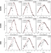 |
Fig. 1. Histograms of the normalised occurrence (black circles) and κ-Gaussian distributions (red lines) of the (from left to right) total, perpendicular, and parallel γ. From top to bottom: SCSW, FCSW, and HSS for all the SIR events on our list. The Pearson R and the root mean square error (RMSE) of the fitted κ-Gaussian versus the normalised histogram values are shown at the top of each panel. |
The weighted κ-Gaussian fit in the case of the FCSW (middle-left panel in Fig. 1) resulted in a nearly adiabatic  of ≈1.73 (assuming plasma with three degrees of freedom), while the partial polytropic index in the perpendicular and parallel direction has a
  of ≈1.62 and a
  of ≈1.81. The increase in
  is accompanied by an increase in both temperature anisotropy and plasma β (from 0.89 in the SCSW to 1.01 in the FCSW and from 0.53 to 0.74, respectively). The
  of the HSS, on the other hand, increased even more, to ≈1.86 (middle-left panel in Fig. 1), while the partial polytropic index in the perpendicular and parallel direction had a
  of ≈1.97 and a
  of ≈2.13. The super-adiabatic effective polytropic index in the HSS is accompanied by a small increase in the average temperature anisotropy and a decrease in the average plasma β (α ≈ 1.04 and β ≈ 0.64) compared to the FCSW.
We further investigated the dependence of the effective polytropic index during the HSS for different solar wind speed levels. Figure D.2 shows the weighted κ-Gaussian fit in the case of VSW > 500 km/s, VSW > 550 km/s, and VSW > 600 km/s. As shown, there is a gradual decrease in the effective polytropic index (left panels in Fig. D.2) as we isolate HSS intervals with increasing solar wind speed, from an average  of ≈1.86 in the entire HSS (VSW > 450 km/s) to an average
  of ≈1.49 in the very fast HSS (VSW > 600 km/s). This significant decrease in the effective polytropic index, from super-adiabatic to sub-adiabatic values, is accompanied by an increase in both temperature anisotropy (from α ≈ 1.04 to α ≈ 1.22) and plasma β (from β ≈ 0.64 to β ≈ 0.81).
4. Discussion
Our results regarding the polytropic behaviour of SIR and HSS are summarised in Table 1 and Fig. 2. The SCSW region contains more turbulent plasma compared to the FCSW and HSS (Tsurutani et al. 2006). This is also depicted in the sub-adiabatic values of the effective polytropic index, which are indicative of turbulent heating for three effective degrees of freedom. In contrast, the FCSW, comprising less compressed and faster plasma, has a near-adiabatic effective γ. However, both SIRs have decreased and increased partial γ in the perpendicular and parallel directions (with respect to the local magnetic field), respectively, (red and green lines in the left panel in Fig. 2). This is in agreement with the results of Katsavrias et al. (2024b), according to whom this variation is a result of the variation in the effective degrees of freedom (deff) in the corresponding direction (a decrease in deff leads to an increase in the effective γ and vice versa). Furthermore, this behaviour seems to be typical for compressed and/or turbulent regions like interplanetary coronal mass ejection sheaths (see also Fig. 7 in Katsavrias et al. 2025a).
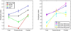 |
Fig. 2. Comparison of the total and partial polytropic index for the various SIRs and HSSs. Left panel: Entire Wind dataset (from Katsavrias et al. 2024b), SCSW, FCSW, and HSS in black, red, green, and blue, respectively. Right panel: HSSs with VSW > 450 km/s (blue), VSW > 500 km/s (magenta), VSW > 550 km/s (cyan), and VSW > 600 km/s (yellow). |
Effective  , anisotropy (α), and plasma β values for the various SIR classifications.
The polytropic index of the HSS is, on average, super-adiabatic, unlike the compressed solar wind. Our results indicate that there is a gradual decrease in the average effective γ in HSSs, from super-adiabatic to sub-adiabatic, if we isolate regions of increasing solar wind speed levels. The aforementioned result does not imply a dependence of the effective γ on the solar wind speed, but is rather an effect of the plasma β increase (see also Table 1). This anti-correlation between the effective polytropic index and the plasma β has been shown to be evident in observations from both Wind and Parker Solar Probe (Nicolaou et al. 2020). This dependence on plasma β is further supported by the fact that for increasing solar wind speed values (see the right panel in Fig. 2), the effective  tends to be lower than
  , indicating increased effective degrees of freedom in the parallel direction (Katsavrias et al. 2024b).
Our results for the total polytropic index are in agreement with those from Dayeh et al. (2025), who find that  , 1.66, and 1.77 for the SCSW, the FCSW, and the HSS, respectively. The minor differences between their results and ours can be explained by the different methodologies and SIR lists used in the two studies. Nevertheless, both studies describe a transition from a sub-adiabatic polytropic behaviour in the SCSW to a super-adiabatic in the HSS.
Following Katsavrias et al. (2024a), we further connected the derived polytropic indices with the entropy gradient and the turbulent heating gradient (Livadiotis et al. 2020) at 1 AU (see Appendix C for more details). Figure 3 shows the polytropic and entropy jump for the various SIRs. We assumed an adiabatic solar wind with a  of ≈1.67. This is of course purely theoretical and valid for slow solar wind streams with isotropic temperatures and three effective degrees of freedom. As shown, the entropic gradient jump (Δ(dS/dR)) from the theoretical adiabatic solar wind to the SCSW is ≈0.54, indicative of turbulent heating in compressed solar wind regions, while the entropic gradient jump from the SCSW to the FCSW and then to the HSS is ≈ − 0.84 and −0.27, respectively.
To further investigate the increase in the polytropic index in the HSS, we derived the distribution of the effective total  with respect to the temperature anisotropy and plasma β∥. The top panels in Fig. 4 show the two-dimensional histograms of the data points in the anisotropy–β∥ parameter space. As shown, the HSS exhibits a characteristic tail of high values of α and low values of plasma β∥ (top-right panel in Fig. 4) compared to the SCSW (top-left panel), which exhibits anisotropy values very close to 1. The bottom panels in Fig. 4 show the distribution of the effective total
  in each log10(α)–log10(β∥) bin. The total
  in each bin was derived using a κ–Gaussian fitting (similarly to Figs. 1 and D.2). As shown, the
  of the SCSW is, on average, sub-adiabatic and has a clear dependence on plasma β∥. The γ of the HSS is, on average, super-adiabatic. Furthermore, the maximum
  values, which are limited at log10(β∥) < 10−0.3, appear to be grouped in near-diagonal stripes (dashed white lines in the bottom-right panel in Fig. 4). Interestingly, this feature is very similar to the hodogram of a plasma parcel due to the effect of large-scale compressive slow-mode waves as described in Fig. 2 in Verscharen et al. (2016). Large-amplitude compressive fluctuations, which are a significant component of astrophysical plasma turbulence, lead to changes in the anisotropy and plasma β∥ and, consequently, to the plasma crossing one or more instability thresholds. As a result, energy can be transferred from the large-scale compressions to small-scale kinetic instabilities, which in terms of thermodynamics would result in a net energy loss from the compressions and, thus, a super-adiabatic polytropic index. Dayeh et al. (2025) suggest an additional mechanism that can drive the super-adiabatic value of the polytropic index in the HSS, which is the increasing Alfvén wave activity. A more detailed investigation of these mechanisms and their relative contribution will be revisited in a future work.
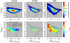 |
Fig. 4. Two-dimensional histograms of the temperature anisotropy with respect to the parallel plasma β (β∥) for the SCSW (left), FCSW (middle), and HSS (right). Overplotted are the mirror (solid lines), proton cyclotron (dotted lines), parallel (dashed lines), and oblique (dot-dashed lines) fire hose instabilities assuming a maximum growth rate of 10−3 (Hellinger et al. 2006). The dotted white line in the top panels corresponds to the most frequent value in each log10(β); the normalised occurrence in each bin is colour-coded, with red corresponding to 1. The bottom panels correspond to the distribution of the effective total |


5. Conclusions
We have performed a detailed investigation of the proton polytropic behaviour in SIRs using a list of 186 events identified from Wind measurements over more than two solar cycles (1995–2002). Our main conclusions are summarised as follows:
-
The SCSW part of SIRs is sub-adiabatic, consistent with turbulent plasma, while the FCSW part of SIRs is near-adiabatic. Both parts of the SIR have lower and higher partial effective
 values in the perpendicular and parallel direction, respectively, consistent with high temperature anisotropy.
 -
As we move to the uncompressed fast solar wind (HSS), the effective polytropic index reaches super-adiabatic values, indicating expansion and/or energy release. This behaviour is consistent with the scenario of large-amplitude compressive fluctuations leading to a net energy loss of the large-scale compression to small-scale instabilities.
-
The effective
 in the HSS decreases to sub-adiabatic values with increasing speed, while the partial effective
  in the parallel direction becomes lower than in the perpendicular direction, consistent with the increase in plasma β values.
 -
Assuming the transition from the theoretically adiabatic solar wind (
 ) to the SCSW, then to the FCSW and HSS and then back to the theoretically adiabatic solar wind, the entropic gradients (dS = dR) are 0.54 [kB/au], −0.84 [kB/au], −0.27 [kB/au], and 0.57 [kB/au], respectively.
The analysis carried out in this work could be extended to in situ measurements closer to the Sun (i.e. from Solar Orbiter and Parker Solar Probe) and thus enable a deeper physical understanding of the role of internal and ambient interactions of an SIR en route to Earth.
Acknowledgments
The authors thank the National Space Science Data Center of the Goddard Space Flight Center for the use permission of Wind data and the NASA CDAWeb team for making these data available at http://cdaweb.gsfc.nasa.gov/istp_public/. DV is supported by STFC Consolidated Grant ST/W001004/1.
References
- Abraham, J. B., Verscharen, D., Wicks, R. T., et al. 2022, ApJ, 941, 145 [NASA ADS] [CrossRef] [Google Scholar]
- Arridge, C., McAndrews, H., Jackman, C., et al. 2009, PSS, 57, 2032 [Google Scholar]
- Borovsky, J. E., & Denton, M. H. 2006, J. Geophys. Res., 111 [Google Scholar]
- Chandrasekhar, S. 1957, An Introduction to the Study of Stellar Structure, Astrophysical Monographs (Dover Publications) [Google Scholar]
- Dakeyo, J.-B., Maksimovic, M., Démoulin, P., Halekas, J., & Stevens, M. L. 2022, ApJ, 940, 130 [NASA ADS] [CrossRef] [Google Scholar]
- Dayeh, M. A., & Livadiotis, G. 2022, ApJ, 941, L26 [NASA ADS] [CrossRef] [Google Scholar]
- Dayeh, M. A., Starkey, M. J., Livadiotis, G., et al. 2025, ApJ, 984, L33 [Google Scholar]
- Denton, M. H., & Borovsky, J. E. 2012, J. Geophys. Res., 117, A9 [Google Scholar]
- Dialynas, K., Roussos, E., Regoli, L., et al. 2018, J. Geophys. Res., 123, 8066 [NASA ADS] [CrossRef] [Google Scholar]
- Elliott, H. A., McComas, D. J., Zirnstein, E. J., et al. 2019, ApJ, 885, 156 [Google Scholar]
- Grandin, M., Aikio, A. T., & Kozlovsky, A. 2019, J. Geophys. Res., 124, 3871 [Google Scholar]
- Hellinger, P., Trávnícek, P., Kasper, J. C., & Lazarus, A. J. 2006, GRL, 33, 9 [Google Scholar]
- Horne, R. B., Phillips, M. W., Glauert, S. A., et al. 2018, Space Weather, 16, 1202 [CrossRef] [Google Scholar]
- Jian, L., Russell, C. T., Luhmann, J. G., & Skoug, R. M. 2006, Sol. Phys., 239, 337 [NASA ADS] [CrossRef] [Google Scholar]
- Kartalev, M., Dryer, M., Grigorov, K., & Stoimenova, E. 2006, J. Geophys. Res., 111, A10 [Google Scholar]
- Katsavrias, C. 2025, https://doi/10.5281/zenodo.15225254 [Google Scholar]
- Katsavrias, C., Hillaris, A., & Preka-Papadema, P. 2016, ASR, 57, 22342244 [Google Scholar]
- Katsavrias, C., Sandberg, I., Li, W., et al. 2019, J. Geophys. Res., 124, 4402 [Google Scholar]
- Katsavrias, C., Nicolaou, G., Di Matteo, S., et al. 2024a, A&A, 686, L10 [NASA ADS] [CrossRef] [EDP Sciences] [Google Scholar]
- Katsavrias, C., Nicolaou, G., & Livadiotis, G. 2024b, A&A, 691, L11 [NASA ADS] [CrossRef] [EDP Sciences] [Google Scholar]
- Katsavrias, C., Nicolaou, G., Livadiotis, G., et al. 2025a, A&A, 695, A146 [NASA ADS] [CrossRef] [EDP Sciences] [Google Scholar]
- Katsavrias, C., Di Matteo, S., Kepko, L., & Viall, N. M. 2025b, A&A, 696, L20 [NASA ADS] [CrossRef] [EDP Sciences] [Google Scholar]
- Kilpua, E. K. J., Hietala, H., Turner, D. L., et al. 2015, GRL, 42, 3076 [Google Scholar]
- Kuhn, S., Kamran, M., Jelic, N., et al. 2010, AIP Conference Proceedings (AIP), 1306, 216 [Google Scholar]
- Lepping, R. P., Acũna, M. H., Burlaga, L. F., et al. 1995, Space Sci. Rev., 71, 207 [Google Scholar]
- Livadiotis, G. 2015, ApJ, 809, 111 [NASA ADS] [CrossRef] [Google Scholar]
- Livadiotis, G. 2016, ApJS, 223, 13 [NASA ADS] [CrossRef] [Google Scholar]
- Livadiotis, G. 2018a, Entropy, 20, 799 [NASA ADS] [CrossRef] [Google Scholar]
- Livadiotis, G. 2019a, Stats, 2, 416 [CrossRef] [Google Scholar]
- Livadiotis, G. 2019b, Entropy, 21, 1041 [NASA ADS] [CrossRef] [Google Scholar]
- Livadiotis, G. 2021, Res. Notes AAS, 5, 4 [Google Scholar]
- Livadiotis, G., & McComas, D. J. 2011, ApJ, 741, 88 [NASA ADS] [CrossRef] [Google Scholar]
- Livadiotis, G., & McComas, D. J. 2013, J. Geophys. Res., 118, 2863 [NASA ADS] [CrossRef] [Google Scholar]
- Livadiotis, G., & McComas, D. J. 2023, Sci. Rep., 13, 9033 [NASA ADS] [CrossRef] [Google Scholar]
- Livadiotis, G. P., Dayeh, M. A., & Zank, G. 2020, ApJ, 905, 137 [NASA ADS] [CrossRef] [Google Scholar]
- Miyoshi, Y., & Kataoka, R. 2008, J. Geophys. Res., 113, A3 [Google Scholar]
- Nasi, A., Katsavrias, C., Daglis, I. A., et al. 2022, Front. Astron. Space Sci., 9 [Google Scholar]
- Newbury, J. A., Russell, C. T., & Lindsay, G. M. 1997, GRL, 24, 1431 [NASA ADS] [CrossRef] [Google Scholar]
- Nicolaou, G., & Livadiotis, G. 2019a, ApJ, 884, 52 [NASA ADS] [CrossRef] [Google Scholar]
- Nicolaou, G., Livadiotis, G., & Moussas, X. 2014a, Sol. Phys., 289, 1371 [NASA ADS] [CrossRef] [Google Scholar]
- Nicolaou, G., Livadiotis, G., & Wicks, R. T. 2019b, Entropy, 21, 997 [NASA ADS] [CrossRef] [Google Scholar]
- Nicolaou, G., Livadiotis, G., Wicks, R. T., Verscharen, D., & Maruca, B. A. 2020, ApJ, 901, 26 [CrossRef] [Google Scholar]
- Nicolaou, G., Livadiotis, G., & Desai, M. I. 2021, Appl. Sci., 11, 4643 [Google Scholar]
- Nicolaou, G., Livadiotis, G., & McComas, D. J. 2023, ApJ, 948, 22 [CrossRef] [Google Scholar]
- Ogilvie, K. W., Chornay, D. J., Fritzenreiter, R. J., et al. 1995, Space Sci. Rev., 71, 55 [Google Scholar]
- Parker, E. 1963, Interplanetary Dynamical Processes, InterscienceMonographs and Texts in Physics and Astronomy (Interscience Publishers) [Google Scholar]
- Scherer, K., Fichtner, H., Fahr, H. J., Röken, C., & Kleimann, J. 2016, ApJ, 833, 38 [NASA ADS] [CrossRef] [Google Scholar]
- Siegel, A. F. 1982, Biometrika, 69, 242 [NASA ADS] [CrossRef] [Google Scholar]
- Tsurutani, B. T., Gonzalez, W. D., Gonzalez, A. L. C., et al. 2006, J. Geophys. Res., 111, A7 [Google Scholar]
- Turner, D. L., Kilpua, E. K. J., Hietala, H., et al. 2019, J. Geophys. Res., 124, 1013 [NASA ADS] [CrossRef] [Google Scholar]
- Verma, M. K., Roberts, D. A., & Goldstein, M. L. 1995, J. Geophys. Res., 100, 19839 [NASA ADS] [CrossRef] [Google Scholar]
- Verscharen, D., Chandran, B. D. G., Klein, K. G., & Quataert, E. 2016, ApJ, 831, 128 [NASA ADS] [CrossRef] [Google Scholar]
Appendix A: SIR list
The SIR list used in this study is a refinement and extension of the Grandin et al. (2019) list. In detail, we have excluded all events that had embedded coronal mass ejections and kept only single and isolated events without preconditioning, requiring the average solar wind speed and number density to be less than 400 km/s and 15 cm−3, respectively, for at least 12 hr before the start of the event. The start and end time of the interaction region is identified as the time period where the density increases above 10 particles/cm−3, accompanied by an increase in the IMF magnitude and the proton density gradient (dnp/dt). Similarly, the HSS start time is identified as the time when solar wind speed exceeds 450 km/s, while the HSS end time corresponds to the first time when the solar wind speed drops below 400 km/s after reaching its maximum value. Figure D.1 shows an example of an SIR event on our list.
Appendix B: Derivation of the polytropic index
The steps towards a valid derivation of γ, were first introduced in Katsavrias et al. (2024a) and are summarised below:
-
We analysed sufficiently short sub-intervals, using a sliding window of ≈10 min, in order to minimise the possibility of mixing measurements of different streamlines (Kartalev et al. 2006; Livadiotis 2018a; Nicolaou & Livadiotis 2019a).
-
In each sub-interval, we performed a repeated median regression (Siegel 1982), which is a variation of the Theil–Sen estimator, to the logarithm of the right hand side of Eq. 1 for solar wind protons. The repeated median regression offers a more robust option over the more common least-squares linear fit, given the small number of data points per window. It is also much less sensitive to outliers.
-
We further examined the stability of Bernoulli’s integral (again at each sub-interval) by requiring the standard deviation over the mean to be less than 2%. This condition is particularly important, as it enhances the possibility that the analysed sub-intervals correspond to individual streamlines, where the polytropic relation is valid (Kartalev et al. 2006). We note that we have ignored the contribution of electrons in the estimation of the Bernoulli’s integral. Nevertheless, we expect negligible differences since the contribution of the thermal pressure to the Bernoulli’s integral near L1 is very small compared to the dynamic pressure term (Nicolaou et al. 2021).
-
We further filtered the derived polytropic indices by requiring a) the Pearson correlation coefficient of the regressed versus the measured data points to be higher than 0.8 and b) each special polytropic index (vinv), which corresponds to the inverse spectrum regression (see also Nicolaou et al. 2019b; Livadiotis 2019a) to differ no more than 0.1 from the corresponding γ.
We further determined the average anisotropy and plasma β values as well as solar wind bulk speed for each ten-minute sub-interval, in order to examine possible correlations between them. The estimation of γ by fitting in lnT versus lnn is much more straightforward since it is based directly on measured quantities (Newbury et al. 1997; Kartalev et al. 2006). In contrast, fitting in lnP versus lnn would result in artifacts (biased correlations due to the fact that P is constructed from the measured n, thus not independently measured), and furthermore, the error propagation would result in significantly higher uncertainty.
Finally, following Livadiotis & McComas (2011) and Nicolaou et al. (2014a), we fitted a κ-Gaussian distribution given by
![Mathematical equation: $$ \begin{aligned} f(\gamma ,\overline{\gamma },\kappa _{0},\sigma ) \propto \left[ 1 + \frac{\left( \gamma - \overline{\gamma }\right)^{2}}{\kappa _{0}\cdot \sigma ^{2}} \right]^{-\kappa _{0}-3/2}, \end{aligned} $$](/articles/aa/full_html/2025/09/aa56105-25/aa56105-25-eq37.gif) (B.1)
(B.1)
where  is the average polytropic index. We emphasise that the fitting was performed on the enriched γ histograms, which allow for both the binned values and their uncertainties to be taken into account. Specifically, for each γ (and after the filtering discussed in the previous section), we generated a normally distributed set of 1000 values with a mean and sigma values corresponding to the original value and its uncertainty (see also Livadiotis 2016, and discussion therein).
Appendix C: Connection of the polytropic index to the entropy gradient
The proton entropy can be expressed in terms of proton density and temperature (Livadiotis 2019b, 2021) as
 (C.1)
(C.1)
where S is the Boltzmann-Gibbs entropic measure, deff are the effective degrees of freedom, n is the number density, and kB the Boltzmann constant (Livadiotis & McComas 2023). Furthermore, the density drop can be approximated as
 (C.2)
(C.2)
where R is the radial distance, while the polytropic relation for isotropic temperature is
 (C.3)
(C.3)
Combining Eqs. C.1, C.2, and C.3, we obtain
 (C.4)
(C.4)
where γα = 1 + 2/deff so that deff = 3 and γα = 5/3. Combining these equations, we express the entropy gradient as
 (C.5)
(C.5)
On the other hand, the gradient of the turbulent heating Et of the proton plasma (per mass), normalised by the thermal energy, is also equal to the deviation of the polytropic index from its adiabatic value (Verma et al. 1995; Livadiotis 2019a,b),
 (C.6)
(C.6)
The adiabatic polytropic index can be written as a function of the effective kinetic degrees of freedom as γα = 1 + 2/deff. Assuming that deff = 3 and γα = 5/3, the entropic gradient jump is three times the polytropic jump. Here we have assumed a constant γα, ignoring its dependence in anisotropy (Katsavrias et al. 2024a). However, the average change in γα due to the anisotropy change in the SCSW–FCSW–HSS transition (see also table 1) is less than 1% and therefore can be neglected.
Appendix D: Supplementary figures
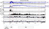 |
Fig. D.1. Example of an SIR event on November 2008. From top to bottom: IMF and its z component (black and blue lines, respectively), proton number density and solar wind bulk speed (black and blue lines, respectively), proton density gradient, solar wind speed gradient, temperature anisotropy, and plasma β. The vertical dashed red lines show the SIR start and end time as well as the HSS end time. |
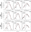 |
Fig. D.2. Same as Fig. 1 but for different solar wind speed levels inside the HSS. From top to bottom: VSW> 500 km/s, VSW> 550 km/s, and VSW> 600 km/s. |
All Tables
Effective , anisotropy (α), and plasma β values for the various SIR classifications.
All Figures
|
Fig. 1. Histograms of the normalised occurrence (black circles) and κ-Gaussian distributions (red lines) of the (from left to right) total, perpendicular, and parallel γ. From top to bottom: SCSW, FCSW, and HSS for all the SIR events on our list. The Pearson R and the root mean square error (RMSE) of the fitted κ-Gaussian versus the normalised histogram values are shown at the top of each panel. |
| In the text | |
|
Fig. 2. Comparison of the total and partial polytropic index for the various SIRs and HSSs. Left panel: Entire Wind dataset (from Katsavrias et al. 2024b), SCSW, FCSW, and HSS in black, red, green, and blue, respectively. Right panel: HSSs with VSW > 450 km/s (blue), VSW > 500 km/s (magenta), VSW > 550 km/s (cyan), and VSW > 600 km/s (yellow). |
| In the text | |
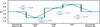 |
Fig. 3. Estimated polytropic and entropic gradient jumps according to Eq. (C.6) at 1 AU. |
| In the text | |
|
Fig. 4. Two-dimensional histograms of the temperature anisotropy with respect to the parallel plasma β (β∥) for the SCSW (left), FCSW (middle), and HSS (right). Overplotted are the mirror (solid lines), proton cyclotron (dotted lines), parallel (dashed lines), and oblique (dot-dashed lines) fire hose instabilities assuming a maximum growth rate of 10−3 (Hellinger et al. 2006). The dotted white line in the top panels corresponds to the most frequent value in each log10(β); the normalised occurrence in each bin is colour-coded, with red corresponding to 1. The bottom panels correspond to the distribution of the effective total |
| In the text | |
|
Fig. D.1. Example of an SIR event on November 2008. From top to bottom: IMF and its z component (black and blue lines, respectively), proton number density and solar wind bulk speed (black and blue lines, respectively), proton density gradient, solar wind speed gradient, temperature anisotropy, and plasma β. The vertical dashed red lines show the SIR start and end time as well as the HSS end time. |
| In the text | |
|
Fig. D.2. Same as Fig. 1 but for different solar wind speed levels inside the HSS. From top to bottom: VSW> 500 km/s, VSW> 550 km/s, and VSW> 600 km/s. |
| In the text | |
Current usage metrics show cumulative count of Article Views (full-text article views including HTML views, PDF and ePub downloads, according to the available data) and Abstracts Views on Vision4Press platform.
Data correspond to usage on the plateform after 2015. The current usage metrics is available 48-96 hours after online publication and is updated daily on week days.
Initial download of the metrics may take a while.