| Issue |
A&A
Volume 701, September 2025
|
|
|---|---|---|
| Article Number | A287 | |
| Number of page(s) | 9 | |
| Section | Atomic, molecular, and nuclear data | |
| DOI | https://doi.org/10.1051/0004-6361/202556110 | |
| Published online | 25 September 2025 | |
Broadband spectroscopy of astrophysical ice analogues
III. Scattering properties and porosity of CO and CO2 ices
1
Prokhorov General Physics Institute of the Russian Academy of Sciences,
119991
Moscow,
Russia
2
Max-Planck-Institut für Extraterrestrische Physik,
Gießenbachstraße 1,
Garching
85748,
Germany
3
Department of Engineering Physics, Polytechnique Montréal,
Montreal,
Quebec,
H3C 3A7,
Canada
★ Corresponding author: This email address is being protected from spambots. You need JavaScript enabled to view it.
Received:
26
June
2025
Accepted:
12
August
2025
Abstract
Context. The quantification of the terahertz (THz) and IR optical properties of astrophysical ice analogs, which have different molecular compositions, phases, and structural properties, is required to model both the continuum emission by the dust grains covered with thick icy mantles and the radiative transfer in the dense cold regions of the interstellar medium.
Aims. We developed a model to define a relationship between the THz-IR response and the ice porosity. It includes the reduced effective optical properties of porous ices and the additional wave extinction due to scattering on pores. The model is applied to analyze the measured THz-IR response of CO and CO2 laboratory ices and to estimate their scattering properties and porosity.
Methods. Our model combines the Bruggeman effective medium theory, the Lorentz-Mie and Rayleigh scattering theories, and the radiative transfer theory to analyze the measured THz-IR optical properties of laboratory ices.
Results. We apply this model to show that the electromagnetic-wave scattering in studied laboratory ices occurs mainly in the Rayleigh regime at frequencies below 32 THz. We conclude that pores of different shapes and dimensions can be approximated by spheres of effective radius. By comparing the measured broadband response of our laboratory ices with those of reportedly compact ices from earlier studies, we quantify the scattering properties of our CO and CO2 ice samples. Their porosity is shown to be as high as 15 and 22%, respectively. Underestimating the ice porosity in the data analysis leads to a proportional relative underestimate of the THz-IR optical constants.
Conclusions. The scattering properties and porosity of ices have to be quantified along with their THz-IR response in order to adequately interpret astrophysical observations. The developed model paves the way for solving this demanding problem of laboratory astrophysics.
Key words: astrochemistry / methods: laboratory: solid state / techniques: spectroscopic / ISM: clouds / dust, extinction
The two authors contributed equally to this work.
© The Authors 2025
 Open Access article, published by EDP Sciences, under the terms of the Creative Commons Attribution License (https://creativecommons.org/licenses/by/4.0), which permits unrestricted use, distribution, and reproduction in any medium, provided the original work is properly cited.
This article is published in open access under the Subscribe to Open model.
Open Access funding provided by Max Planck Society.
1 Introduction
Solving many problems in astrophysics and astrochemistry requires knowledge of the physical properties of interstellar and circumstellar ices (Boogert et al. 2015). These problems include, in particular, the evolution of molecular clouds and the formation of stellar systems (Dominik & Tielens 1997; Öberg & Bergin 2021; Caselli et al. 2022), and the formation of new molecular species in space and their abundances (Mifsud et al. 2021a; Jørgensen et al. 2020; Mifsud et al. 2021b). Measurements of the continuum emission in the millimeter, terahertz (THz), and far-IR ranges (Jørgensen et al. 2020; Widicus Weaver 2019) are major sources of observational data for astrophysical ices. Hence, there is a need for equivalent laboratory measurements and the resulting databases of broadband optical properties for different analogs of interstellar and circumstellar ices, including water (H2O), carbon monoxide (CO), and carbon dioxide (CO2), as well as a few other main constituents and their mixtures (Widicus Weaver 2019; Giuliano et al. 2019; Gavdush et al. 2022; Allodi et al. 2014; Ioppolo et al. 2014; McGuire et al. 2016).
Most of the ongoing laboratory research is concentrated on studying astrophysical ice analogs of different compositions, while substantially fewer efforts have been put into obtaining information on structural features, such as porosity. These features depend on the experimental methodology of growing ice films, including different approaches and conditions (i.e., temperature, pressure, growth rate, etc.) of depositing ice on a cold substrate from the gas phase (Cartwright et al. 2008; Loeffler et al. 2016; Millán et al. 2019). Annealing at different temperatures affects the structure of ice samples, promoting phase transition (Isokoski et al. 2014; Cazaux et al. 2015; Schiltz et al. 2024). In the laboratory, the thickness of ice samples is usually varied between ~100 nm and 10 µm for IR measurements, and from ~10 µm to 1 mm for THz and millimeter measurements, with the aim of ensuring the spectroscopic measurements are sufficiently sensitive (Gavdush et al. 2022). Ice porosity generally increases with the thickness, ranging from several to tens of percent by volume (Millán et al. 2019; Loeffler et al. 2016; Westley et al. 1998). High porosity impacts the THz-IR response of laboratory ices, leading to a reduction in the effective optical constants (Millán et al. 2019; Loeffler et al. 2016), a broadening of absorption peaks, and a reduction in their amplitude (Loeffler et al. 2016; Schiltz et al. 2024), or even to the dielectric spectrum redistribution and formation of additional absorption bands due to crystalline lattice disordering, such as the Boson peaks (Gavdush et al. 2022; Lunkenheimer & Loidl 2003; Dyre & Schrøder 2000). At higher frequencies, porosity induces a strong scattering of electromagnetic waves, which makes ice samples optically opaque. This effect restrains the spectral range of ice characterization, leading to profound differences between the THz-IR responses of compact and porous samples, which should be taken into account in both laboratory measurements and subsequent calculations of radiative transfer in the interstellar medium (ISM; Mitchell et al. 2017; Rocha et al. 2024; Schiltz et al. 2024).
While it is broadly believed that porous ices are rare in the ISM (Keane et al. 2001) because of their thermal annealing, exposure to cosmic rays and vacuum ultraviolet, or H-atom bombardment (Palumbo 2006; Raut et al. 2007, 2008; Palumbo et al. 2010; Accolla et al. 2011), there is still no complete consensus on this issue. Relying on the available observations, it is challenging to determine the actual porosity of interstellar and circumstellar ices. Among the main arguments in favor of compact ices is the common absence of dangling OH features, which trace unbound water molecules. However, some laboratory data have also revealed the absence of such modes for porous samples (Raut et al. 2007; Isokoski et al. 2014; He et al. 2022). At the same time, the recent work by Noble et al. (2024) shows a detection of the dangling OH features with the JWST NIRCam in Chamaeleon I, which could be an indication of a porous ice structure.
If porous ices were present in the ISM, their structural properties would play an important role in a number of processes, such as accretion, desorption, segregation, and diffusion. Because of the larger effective surface area, porous ices are expected to be more chemically reactive, enabling the trapping of volatiles and the freezing out of additional atoms and molecules. The possible existence of porous ices in the ISM would stimulate the formation of various complex organic molecules, photodesorption processes (Öberg et al. 2009b,a; Fayolle et al. 2011), and exothermic solid-state reactions (Cazaux et al. 2010; Dulieu et al. 2013). Thereby, knowledge of the structural features and porosity of ices from laboratory experiments, as well as from the related models of their dielectric response, is needed to assist in the interpretation of astronomical observations (Westley et al. 1998; Accolla et al. 2011; Bossa et al. 2014; Isokoski et al. 2014; Loeffler et al. 2016; Millán et al. 2019; Rocha et al. 2024).
A few available works on the porosity of astrophysical ice analogs present results for H2O, CO, CO2, and their mixtures. Often, a quartz-crystal microbalance is used to estimate the density of ices, while interferometry is applied to quantify their refractive index in the visible and near-IR ranges (Westley et al. 1998; Loeffler et al. 2016; Millán et al. 2019). For this purpose, information about the density and refractive index of bulk is usually taken from the literature (Maass & Barnes 1926; Schulze & Abe 1980; Warren 1986; Westley et al. 1998; Dohnálek et al. 2003). Another option is to use diffraction measurements to directly obtain the density of bulk regions in a porous sample (Millán et al. 2019). Although the effective medium theory (EMT) makes it possible to estimate porosity from spectroscopic data (Bossa et al. 2014; Millán et al. 2019), it requires a priori knowledge of the properties of compact ices, typically taken from the literature. Additional IR measurements can be applied to check the specific modes expected for porous ices (Bossa et al. 2014; Isokoski et al. 2014; Mitchell et al. 2017; Nagasawa et al. 2021; Rocha et al. 2024). Less frequently, scanning electron microscopy (Cartwright et al. 2008), Monte Carlo simulations (Cazaux et al. 2015; Clements et al. 2018), and other experimental and theoretical techniques are applied to study the morphology of laboratory ices.
This series of papers is focused on measurements and analysis of the broadband optical properties of laboratory ices. In Giuliano et al. (2019), we developed the experimental setup and methods to grow laboratory ice samples, measure their THz complex transmission (using the THz pulsed spectrometer), and retrieve their THz optical properties from the measured data. In Gavdush et al. (2022), we describe the method for merging the data of THz pulsed spectroscopy and Fourier-transform IR (FTIR) spectroscopy for the broadband characterization of ices, which was then applied to study the THz-IR response of CO and CO2 ices. In these broadband measurements, the high-frequency edge of the analyzed spectral bands was limited to 12 THz (Gavdush et al. 2022); higher frequencies were excluded from the analysis due to monotonically increasing extinction, attributed to scattering. Also, for both CO and CO2 ices, we observe low-intensity absorption peaks at higher frequencies that originate from a disordered crystal lattice and disappear upon annealing (Gavdush et al. 2022). These spectroscopic features further motivated our research into the effects of scattering and porosity.
In the present paper, we develop a model to derive the relationship between the THz-IR optical properties of ices and their porosity. A combined use of the Bruggeman EMT, Lorentz-Mie, and Rayleigh scattering theories, as well as the radiative transfer theory, enabled the characterization of both the reduced effective optical properties of porous ices (occurring at all frequencies) and the additional wave extinction due to scattering on pores (which increases with frequency). This model shows that scattering in the studied ice samples occurs mainly in the Rayleigh regime for frequencies of up to 32 THz. We conclude that pores of different shapes and dimensions can be approximated by spheres of effective radius. The scattering properties and porosity were determined by comparing the measured broad-band response of our CO and CO2 laboratory ices with the literature data on reportedly compact ices. The porosity of the CO and CO2 ice samples in our experiments is about 15% and 22%, respectively. Neglecting the porosity in the data analysis leads to a proportional underestimate of the optical properties.
2 Methods
2.1 THz-IR data on porous CO and CO2 ices
To analyze scattering characteristics and porosity of CO and CO2 ices, we used their THz-IR optical properties as reported by Gavdush et al. (2022) for a limited spectral range below 12 THz. In the present study, we extended the spectral range to 32 THz, which allowed us to take scattering fingerprints into account. Details on the ice growth process and THz-IR measurements are presented in Giuliano et al. (2019) and Gavdush et al. (2022).
Given the apparent scattering signatures seen in the collected data, we concluded that the studied ices are porous and thus kept in mind the following two main effects peculiar to porous analytes:
In the entire spectral range, porous samples possess reduced refractive index and absorption coefficient (compared to that of a compact sample). These are referred to as the effective optical properties commonly defined within the EMT theory (Niklasson et al. 1981; Smolyanskaya et al. 2018; Millán et al. 2019).
The scattering increases monotonically with frequency until the analyte becomes opaque. The total extinction is usually defined as a superposition of the power absorption and scattering coefficients, µtotal = µα + µs (Bohren & Huffman 1998).
Below we treat the THz-IR results reported earlier for CO and CO2 ices as effective optical constants of the respective compact ices, and summarize the methods to describe the aforementioned effects and to quantify the scattering properties, porosity, and effective pore radius of ices.
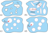 |
Fig. 1 Pores of arbitrary shapes (a) can be approximated by spheroids (b) or spheres (c) of different sizes, or spheres of the same effective radius, Reff (d). |
2.2 The Bruggeman EMT model
Following our previous papers (Giuliano et al. 2019; Gavdush et al. 2022), we describe the THz-IR response of ices by the refractive index (n) and absorption coefficient α (by field). These are related to the complex refractive index ñ = n′ − in″and complex dielectric permittivity  via
via  , where n ≡ n′, v is the frequency, and c0 is the speed of light in vacuum. We point out that the power absorption coefficient (within the radiative transfer theory) is given by µα = 2α.
To define a relation between the compact and porous analytes at a given THz-IR frequency, we used the Bruggeman EMT model (Bruggeman 1935), derived for the optically isotropic two-component mixtures of compact host medium and sub-wavelength (≪ λ) spheres. Although this model is considered to be applicable for spherical particles with the volume fraction of 1/3 ≤ P ≤ 2/3 (Bergman 1982; Smolyanskaya et al. 2018), it appears to be relevant also for particles of a more complex shape and a wider range of volume fractions (up to 0 ≤ P ≤ 1). In particular, the model was shown to be suitable for describing the dielectric response of complex biological objects (Chernomyrdin et al. 2021) and porous materials (Sela & Haspel 2020; Ulitko et al. 2020; Chapdelaine et al. 2022). Also, it can be extended to describe the response of multicomponent systems (Smolyanskaya et al. 2018). If an analyzed medium is a compact material filled with empty pores, Fig. 1a, the model is given by
 (1)
(1)
where  is the effective complex dielectric permittivity of a porous medium, ɛpore = 1 is the dielectric permittivity of pores (empty space) and P is their volume fraction, while
  is the dielectric permittivity of the compact material.
In fact, considering some prior knowledge on the structural properties of an analyte, one can also apply other EMT models of complex dielectric permittivity (Golovan et al. 2007; Smolyanskaya et al. 2018), such as the Maxwell-Garnett (Markel 2016) and Landau-Lifshitz-Looyenga (Landau & Lifshitz 1984; Looyenga 1965) approximations, equation for porous composites proposed by Bergman (1982), and simple linear decomposition of dielectric spectra (Yamaguchi et al. 2016). At a level set by typical ~1% confidence interval for spectroscopic measurements, predictions of these EMT models are very close for a wide range of dimensions, dielectric constants, and volume fractions of scatterers, with the Bruggeman and Landau-Lifshitz-Looyenga models providing somewhat better fits (Millán et al. 2019; Hernandez-Cardoso et al. 2020). Dealing with optically anisotropic media, one can apply the approximation of elliptical particles (Polder & van Santeen 1946) or Lichtenecker model (Lichtenecker 1926; Lichtenecker & Rother 1931; Simpkin 2010), since structural anisotropy and the resulting birefringence can considerably affect the measured data (Chen et al. 2021; Chen & Pickwell-MacPherson 2022; Chernomyrdin et al. 2023).
2.3 Modeling THz-IR scattering in ices
Laboratory ices deposited from gas phase on a cold substrate are intrinsically porous. The structure of pores is generally quite complex and their dimensions can vary broadly, as sketched in Fig. 1a. A prior knowledge or assumptions about characteristic size and volume fraction of pores as well as about the dielectric contrast between the pores and compact ice are required to adequately select the level of simplification and then accurately model the radiative transfer. Geometry of pores is commonly simplified to spheroids or spheres of different dimensions; see Figs. 1b and 1c, respectively.
Although our knowledge on the porosity of ices is limited, some robust assumptions can be introduced.
First, laboratory ices are usually transparent in a wide spectral range spanning the THz and IR bands, down to the wavelengths of λ ~ 1–10 µm (Gavdush et al. 2022). This implies fairly small pores compared to the wavelength scale (Rpore ≪ λ). In such cases, the Rayleigh theory can be applied to accurately describe the scattering properties of ices (Bohren & Huffman 1998).
Second, the average pore size cannot be smaller than the measured diffusion length in the ice. For diffusion of various gases in amorphous solid water ice, this length can be as small as ~10 nm (Furuya et al. 2022), while similar values are expected for ices of other molecular compositions. This exceeds typical scales of ice molecules or crystalline lattices, suggesting the minimum size scale for a single pore.
We assumed the intrinsic absorption of compact ice to be negligible in the spectral range of the scattering analysis (otherwise, the scattering coefficient cannot by rigorously defined; see Mishchenko & Yang 2018; Kucheryavenko et al. 2023). Also, we used the single scattering approximation that is relevant in the case of small volume fractions of pores and low dielectric contrast between the scatterer and the host medium. Then one can write the scattering coefficient µs for a given wavelength in the following form:
 (2)
(2)
where dρ (V) /dV is the unknown volume distribution of pores, Csca (V) = cscaV2 is the Rayleigh scattering cross section with csca describing the wavelength and shape dependence (see Sect. 2.3.1), Vmin and Vmax are the minimum and maximum volumes of pores. Assuming the volume distribution has a power-law spectrum with the exponent −γ, it can be conveniently normalized to the porosity (P; which is the first moment of the distribution),
 (3)
(3)
where condition γ < 2 ensures that the value of P is dominated by bigger pores. Then the scattering coefficient takes the form
 (4)
(4)
where Csca is calculated for a pore of maximum volume Vmax and NV ≡ P/Vmax is the number of such pores per unit volume. Hence, the scattering effects are dominated by larger pores.
We see that, even without a prior knowledge about ice porosity, we can limit our analysis to effective characterization of large-scale pores of the volume  ; see Fig. 1d. For such pores, the scattering coefficient is reduced to the common form (Bohren & Huffman 1998):
 (5)
(5)
where the unknown factor (2 − γ) / (3 − γ) ~ 1 present in Eq. (4) is absorbed in Veff.
Next, we summarize essential facts regarding the Rayleigh and Lorentz-Mie scattering theories and the related approaches to defining scattering parameters that are required to analyze the ice porosity.
2.3.1 Scattering cross section and scattering coefficient based on the Rayleigh approximation
In the Rayleigh limit, the scattering cross section Csca in Eq. (5) depends on the pore polarizability αp as
 (6)
(6)
where k = 2πnbulk/λ is the wavenumber in a bulk medium. For spherical pores of radius Rpore (see Fig. 1c), the polarizability αp is
 (7)
(7)
while for spheroidal pores with semi-axes a, b, c and the equivalent radius (abc)1/3 (see Fig. 1b), it is defined by the polarizability components along the principal axes,
 (8)
(8)
where Li are the corresponding geometrical factors and  . For prolate pores with the semi-axes a > b = c and the geometrical factors L2 = L3, we have
![Mathematical equation: $\eqalign{ & {L_1} = {{1 - {e^2}} \over {{e^2}}}\left[ { - 1 + {1 \over {2e}}\,\ln \left( {{{1 + e} \over {1 - e}}} \right)} \right], \cr & {e^2} = 1 - {{{c^2}} \over {{a^2}}}, \cr} $](/articles/aa/full_html/2025/09/aa56110-25/aa56110-25-eq15.png) (9)
(9)
while for oblate pores with a = b > c and L1 = L2,
 (10)
(10)
For randomly oriented spheroids, the average scattering cross section is given by
 (11)
(11)
In the Rayleigh approximation, the scattering coefficient is proportional to the fourth power of frequency, µs = Av4, where A is a function of the relative dielectric permittivity of compact ice  , the pore shape and size distribution, and the porosity (P). In this way, analysis of experimental spectroscopic data makes it possible to estimate A and thus to obtain information about porosity.
2.3.2 Scattering cross section and scattering coefficient based on rigorous Lorentz-Mie theory
The cross section of a spherical pore of arbitrary radius Rpore (see Fig. 1c) is defined within the general Lorentz-Mie scattering theory (Bohren & Huffman 1998),
 (12)
(12)
where
 (13)
(13)
are the Mie scattering coefficients, ψn(x) and ξn(x) are the Riccati-Bessel functions,  , and x = kRpore. Relying on the Lorentz-Mie cross section, the scattering coefficient µs is usually defined using Eq. (5). We should stress, however, that such a definition should be used cautiously – in fact, it is only applicable if scattering pores are still quite small and their scattering phase functions are overall isotropic (i.e., the Rayleigh-like; see Kucheryavenko et al. 2023). Otherwise, the parameter µs loses its physical meaning and is no longer relevant to describe the radiative transport in porous media.
The limits of applicability of the aforementioned Rayleigh and Lorentz-Mie scattering theories (in terms of the pore sizes and the character of scattering phase function) depend on a number of factors, and are commonly examined experimentally or by numerical analysis (Kucheryavenko et al. 2023).
3 Results
The scattering effects were observed in our previous measurements of CO and CO2 ices at frequencies above v = 12 THz, corresponding to the wavelengths below λ ≈ 25 µm (Gavdush et al. 2022). These ice films were transparent or translucent at frequencies up to v = 32 THz (or at wavelengths down to λ ≈ 9.4 µm). Above the frequency of 18 THz, some narrow frequency bands are excluded from the analysis due to the non-transparency of a beamsplitter in our FTIR spectrometer. Even though quantification of a broadband complex dielectric permittivity based on IR data and the Kramers-Kronig transform (Gavdush et al. 2022) is generally problematic if some spectral fragments are missing, in the present study we obtained robust estimates for the ice scattering coefficient at frequencies up to 32 THz (while neglecting some spectral bands with no FTIR signal and intense absorption by ice). Such scattering can be induced by pores of sizes much smaller than the aforementioned wavelengths, i.e., ≲1 µm, which highlights the need to justify applicability of the Rayleigh scattering regime, as elaborated below.
 |
Fig. 2 Ratio of the Rayleigh scattering cross section of a randomly oriented oblate or prolate spheroid, |


3.1 Approximating pores using effective spheres
Since the actual shape of pores is unknown, we calculated the Rayleigh scattering cross sections Csca for a sphere of volume  and for spheroids with varying c/a ratio but fixed volume
  , equal to that of a sphere. In our analysis, the dielectric permittivity of pores corresponds to that of free space (εpore = 1), while that of bulk host medium is set to εbulk = 2, which is reportedly close to the value for compact CO2 ice (Warren 1986; Gerakines & Hudson 2020).
Figure 2 shows the scattering cross section  of randomly oriented prolate and oblate spheroids, normalized to that of a sphere
  and plotted versus the ratio c/a. We notice that the difference between the scattering cross section of prolate spheroids and a sphere is less than 5% in a wide range of c/a = 0.01–1.0, while that of oblate spheroids and a sphere is less than 10% for c/a = 0.25–1.0. Thus, when such anisotropic pores are randomly oriented, their net contribution is essentially determined by their volume, and the scattering cross section Csca can be reasonably approximated by that of a sphere.
Regarding our laboratory ice films (Gavdush et al. 2022), they were assumed to be isotropic due to the diffuse regime of ice growth, attributed to a sufficiently high deposition pressure in the chamber (Giuliano et al. 2019). This allowed us to exclude any residual anisotropy of pores from our further analysis and treat them as equivalent spheres.
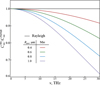 |
Fig. 3 Frequency-dependent ratio of the Lorentz-Mie ( |


3.2 Justifying the Rayleigh scattering regime
Next, we compared the scattering cross section (Csca) of spherical pores of radius Rpore obtained from the Rayleigh (Eqs. (6) and (7)) and Lorentz-Mie [Eqs. (12) and (13)] scattering theories. In Fig. 3, the ratio of the Lorentz-Mie  and Rayleigh
  scattering cross sections is plotted in the frequency range of 0-30 THz for pores of Rpore = 0.4, 0.6, 0.8, and 1 µm. The discrepancy seen between the two theories naturally increases with v and Rpore, which allowed us to describe crossover between the Rayleigh and Mie scattering regimes in our spectral data. For frequencies v < 15 THz, where the discrepancy is less than 10% for Rpore ≤ 0.8 µm, one can claim that the two theories give similar predictions.
The general Lorentz-Mie theory is applicable for arbitrary ratios of the pore radius Rpore and the wavelengths λ, while the Rayleigh approximation only works in the limit of small pores, Rpore ≪ λ. Fortunately, values of the ice dielectric constants as well as ranges of frequencies and pore sizes relevant for our laboratory ices are such that the Rayleigh theory can still be used. In the following, we use it to model the scattering cross section Csca (Eqs. (6) and (7)) and estimate the scattering coefficient µs of laboratory ices (Eq. (5)).
3.3 Porosity, scattering properties, and effective pore radius for laboratory ices
The described methods of the EMT and Rayleigh scattering theory are applied to analyze the scattering properties, effective pore radii (Rpore), and porosity (P) of our CO and CO2 ices (Gavdush et al. 2022). The results are summarized in Fig. 4. We excluded from the analysis the aforementioned spectral bands of low signal (gray-shaded areas), as well as those with resonant absorption peaks (blue-colored areas), attributed to the vibrational modes of ices.
In Fig. 4b we compare the THz-IR refractive index (n) of our CO ices at lower frequencies (≤18 THz) with that at higher frequencies (≳45 THz), reported in Gerakines et al. (2023) for thin compact samples. Taking into account the fact that the refractive index of dielectric materials shows increase with decreasing frequency only while passing the spectral absorption features (as governed by the Kramers-Kronig relations; see Martin 1967), and given the absence of pronounced absorption peaks for CO ice in the frequency gap between 18 and 45 THz, we expect the refractive index of CO ice to be constant within this gap. This allowed us to use the high-frequency refractive index of compact CO ice from Gerakines et al. (2023) to calibrate our THz-IR spectra. In this way, the refractive indices measured at 18 THz and reported at 45 THz are used with the Bruggeman EMT model, Eq. (1), to estimate the porosity of our CO ice: the resulting value is found to be P ≈ 15%. In Fig. 4b we also estimate the broadband refractive index of compact CO ice at lower frequencies ≲18 THz (using our experimental data for porous ice, the retrieved value of porosity, and the Bruggeman model), as well as at higher frequencies (based on the data from Gerakines et al. 2023).
In Fig. 4c we present the absorption coefficient α of our CO ices. The curve increases monotonically with v due to scattering. It is fitted by one half of the scattering coefficient (µs) defined within the Rayleigh formalism,
 (14)
(14)
where A1 is a free parameter that accounts for noise level in our spectroscopic data (Gavdush et al. 2022), while  is also a function of εbulk. The absorption coefficient α (by field) is fitted by µs/2 in order to ensure consistency between our experimental data and the Rayleigh theory. One can see that experimental curve is described well by the model at ≲23 THz, while at higher frequencies a growing deviation becomes evident. The fitting procedure allowed us to quantify the effective pore radius in CO ice, which turned out to be as high as Reff ≈ 0.9 µm. Such large pores cause cross-over between the Rayleigh and Mie scattering regimes at higher frequencies, which explains the origin of the observed deviation.
The results of similar analysis for CO2 ices are presented in Figs. 4e and 4f. Here, substantially more data on the THz–IR refractive index (n) of compact ices were reported earlier (Warren 1986; Baratta & Palumbo 1998; Gerakines & Hudson 2020). In panel e we use the most recent results (Gerakines & Hudson 2020), measured at higher frequencies and overlapping with our spectra in the range of 15–18 THz, which allowed us to calibrate our experimental data and estimate the porosity of our CO2 ice. The derived value is P ≈ 22%, which is even larger than that of our CO ice. In panel f we fit the experimental absorption curve α with the theoretical scattering coefficient µs/2. The resulting effective pore radius of Reff ≈ 0.5 µm is, in turn, smaller than that derived for CO ices. The theory describes our experimental data for CO2 ices well, justifying that scattering occurs in the Rayleigh regime for frequencies below 32 THz – which, in turn, is in overall agreement with Fig. 3.
Summing up, the computed effective pore radii Reff for CO and CO2 ices are in the submicron range, and scattering occurs mostly in the Rayleigh regime. Our estimates for the ice porosity (P) are also quite reasonable, in a range from several to tens of percent, which is typical for laboratory ices deposited from a gas phase on a cold substrate (Millán et al. 2019; Loeffler et al. 2016; Westley et al. 1998).
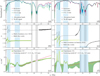 |
Fig. 4 THz-IR optical properties of the studied CO and CO2 ices along with the estimates of scattering parameters. Panel a: examples of the reference and sample IR signals for CO ices. The blue-shaded stripes indicate the absorption bands, and the gray-shaded stripes the ranges of low IR signal. Panels b and c: refractive index (n) and absorption coefficient (α; by field, plotted in log scale) of our CO ices. We show the mean value (solid yellow lines) with the ±1.5σ confidence interval (green shading) for the measurements, as well as the calibrated value for n (dashed black line). The results overlap with the literature data for high-frequency n of compact CO ice from Gerakines et al. (2023), and with the modeled scattering coefficient µs/2, corresponding to P ≈ 15% and Reff ≈ 0.9 µm. Panels d–f: same but for CO2 ices. Here µs/2 corresponds to P ≈ 22% and Reff ≈ 0.5 µm, and the literature data for compact CO2 ice are taken from Gerakines & Hudson (2020). |
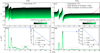 |
Fig. 5 Bruggeman model-based predictions of the THz-IR optical properties of CO and CO2 ices for different values of porosity (P). Panels a and b: refractive index (n) and absorption coefficient (α; by field) of CO ice. Panels c and d: same but for CO2 ice. The inserts in panels b and d depict the maximum amplitude of α for the most intense absorption peak in CO (at 1.5 THz) and CO2 (at 3.5 THz), respectively, plotted versus P. The dashed red rectangles in panels b and d indicate the absorption peaks disappearing upon annealing (presumably caused by the morphological features of porous ice). In panel c, the estimated refractive index of compact (P = 0) CO2 ice is compared with that of reportedly compact samples (Baratta & Palumbo 1998; Gerakines & Hudson 2020). |
3.4 Optical properties of porous and compact laboratory ices
The porosity of P = 15 and 22% derived for our CO and CO2 ices, respectively, makes their responses considerably different from those of compact ices. To quantify this difference for each ice, we modeled the response for P in a range between the respective derived value and P = 0 (compact ice), using the Bruggeman model (Eq. (1)). Color-coded results for n and α are plotted in Fig. 5, showing an evident decrease in both n and α with P. The inserts in panels b and d illustrate the modeled dependences for the most intense absorption peaks in CO (at 1 .5 THz) and CO2 (at 3.5 THz) ices, respectively. The Bruggeman model predicts an almost linear decrease in absorption, which is common for most EMT approximations (Golovan et al. 2007; Smolyanskaya et al. 2018; Markel 2016; Landau & Lifshitz 1984; Looyenga 1965; Bergman 1982; Yamaguchi et al. 2016).
While the EMT has a potential to estimate the ice porosity and predict the optical properties of the bulk, as illustrated in Fig. 5, it does not include several important effects underlying the response of porous samples with disordered crystalline lattice. In fact, the EMT is only able to predict the scaling dependences (Millán et al. 2019; Loeffler et al. 2016), while it does not account for redistribution of the absorption peaks (such as changes in their magnitude, width, shape, and spectral position; see Loeffler et al. 2016; Schiltz et al. 2024) and for the formation of new absorption contours (inherent to disordered systems; see Gavdush et al. 2022; Lunkenheimer & Loidl 2003; Dyre & Schrøder 2000). In Figs. 5b and d, such peaks can be seen near v = 8.11 THz for CO ice, and near v = 7.16 and 8.88 THz for CO2 ice: in Gavdush et al. (2022) they were shown to vanish upon low-temperature annealing, which leads to compaction of ices. We see that our model still recovers these peaks for P = 0, which highlights limitations of the oversimplified EMT approaches.
In Fig. 5c we compare the EMT-based predictions for the refractive index of compact CO2 ice with the high-frequency literature data reported for compact samples (Baratta & Palumbo 1998; Gerakines & Hudson 2020). In contrast to the literature, our experimental curves and the EMT-based predictions do not show the dispersion at 15–18 THz, which is caused by the side lobes of the known vibrational modes of CO2 ice near 20 THz. This apparent discrepancy is simply a result of edge effects in the method applied to derive the optical constants (Gavdush et al. 2022): in the FTIR spectroscopy, the phase information (and, thus, the refractive index of the analyte) is retrieved from the transmission amplitude using the Kramers-Kronig transform. This requires the absorption features to be located well within the spectral range over which the integral is computed – otherwise, the side effects can become dominant.
4 Discussion and conclusion
We have shown that unaccounted for ice porosity can lead to significantly underestimated optical constants in the THz-IR range. Considering the porosity values derived from our experiments as well as from other literature sources reporting on laboratory ices – all in the range between a few to a few dozen percent (Millán et al. 2019; Loeffler et al. 2016; Westley et al. 1998) – we stress that such underestimations should be taken into account when using laboratory data to interpret astrophysical observations.
Our findings highlight the necessity for novel methods and protocols of laboratory ice growth and further thermal processing, which would facilitate ice compaction. Our results also reveal the need for a better understanding the THz-IR response of ices in porous and compact states, including the development of adequate models of broadband complex dielectric permittivity of ices as a function of porosity. Such models would be useful to describe continuum emission and radiative transfer in dense cold regions of the ISM, where thick icy mantles covering dust grains may be porous. Furthermore, porosity may increase with the mantle thickness, which is believed to vary over a broad range, from between a fraction of a nanometer to a fraction of a micron (Boogert et al. 2015), and therefore the broadband optical properties of such mantles could vary dramatically too.
We point out that the method developed to analyze the ice porosity, based on the measured broadband optical properties, is quite generic. It can be useful in both laboratory astrophysics and other fundamental and applied branches of optical spectroscopy involving studies of porous samples.
To summarize, we have developed a model that yields a relationship between the THz-IR responses of compact and porous ices. The model was used to analyze the measured THz-IR response of CO and CO2 laboratory ices, with the aim to estimate their scattering properties and porosity. We have shown that the THz-IR scattering in laboratory ices occurs in the Rayleigh regime, and that the pores of different shapes and dimensions can be approximated by spheres of the same effective radius. By comparing the measured responses of porous CO and CO2 ices with the data available on compact ices, the porosity was found to be as high as ≈15 and ≈22%, respectively. The porosity correction derived in the present paper should be used for the results presented in Giuliano et al. (2019) and Gavdush et al. (2022): neglecting it leads to an almost proportional relative error when estimating the THz-IR optical constants of compact ices. Our findings suggest that the scattering properties and porosity of laboratory ices should be quantified and included in their THz-IR response, to correctly employ these data for interpreting astrophysical observations.
Acknowledgements
A.V.I, B.M.G., and P.C. gratefully acknowledge the support of the Max Planck Society. The work of A.A.G., I.N.D., S.V.G., and K.I.Z. on processing of the THz pulsed spectroscopy and FTIR data, analysis of porosity and scattering properties of ices was supported by the RSF project # 25–79–30006.
References
- Accolla, M., Congiu, E., Dulieu, F., et al. 2011, Phys. Chem. Chem. Phys., 13, 8037 [Google Scholar]
- Allodi, M., Ioppolo, S., Kelley, M., McGuire, B., & Blake, G. 2014, Phys. Chem. Chem. Phys., 16, 3442 [NASA ADS] [CrossRef] [Google Scholar]
- Baratta, G., & Palumbo, M. 1998, JOSAA, 15, 3076 [NASA ADS] [CrossRef] [Google Scholar]
- Bergman, D. 1982, Ann. Phys., 138, 78 [Google Scholar]
- Bohren, C. F., & Huffman, D. R. 1998, Absorption and Scattering of Light by Small Particles (Hoboken: Wiley) [Google Scholar]
- Boogert, A. C. A., Gerakines, P. A., & Whittet, D. C. B. 2015, ARA&A, 53, 541 [Google Scholar]
- Bossa, J.-B., Isokoski, K., Paardekooper, D. M., et al. 2014, A&A, 561, A136 [NASA ADS] [CrossRef] [EDP Sciences] [Google Scholar]
- Bruggeman, D. 1935, Ann. Phys., 416, 636 [NASA ADS] [CrossRef] [Google Scholar]
- Cartwright, J. H. E., Escribano, B., & Sainz-Diaz, C. I. 2008, ApJ, 687, 1406 [Google Scholar]
- Caselli, P., Pineda, J. E., Sipilä, O., et al. 2022, ApJ, 929, 13 [NASA ADS] [CrossRef] [Google Scholar]
- Cazaux, S., Cobut, V., Marseille, M., Spaans, M., & Caselli, P. 2010, A&A, 522, A74 [NASA ADS] [CrossRef] [EDP Sciences] [Google Scholar]
- Cazaux, S., Bossa, J.-B., Linnartz, H., & Tielens, A. G. G. M. 2015, A&A, 573, A16 [NASA ADS] [CrossRef] [EDP Sciences] [Google Scholar]
- Chapdelaine, Q., Nallappan, K., Cao, Y., et al. 2022, Opt. Mater. Express, 12, 3015 [Google Scholar]
- Chen, X., & Pickwell-MacPherson, E. 2022, APL Photonics, 7, 071101 [Google Scholar]
- Chen, X., Sun, Q., Wang, J., Lindley-Hatcher, H., & Pickwell-MacPherson, E. 2021, Adv. Photonics Res., 2, 2000024 [Google Scholar]
- Chernomyrdin, N., Il'enkova, D., Zhelnov, V., et al. 2023, Sci. Rep., 13, 16596 [Google Scholar]
- Chernomyrdin, N. V., Skorobogatiy, M., Gavdush, A. A., et al. 2021, Optica, 8, 1471 [Google Scholar]
- Clements, A. R., Berk, B., Cooke, I. R., & Garrod, R. T. 2018, Phys. Chem. Chem. Phys., 20, 5553 [Google Scholar]
- Dohnálek, Z., Kimmel, G. A., Ayotte, P., Smith, R. S., & Kay, B. D. 2003, J. Chem. Phys., 118, 364 [CrossRef] [Google Scholar]
- Dominik, C., & Tielens, A. G. G. M. 1997, ApJ, 480, 647 [Google Scholar]
- Dulieu, F., Congiu, E., Noble, J., et al. 2013, Sci. Rep., 3, 1338 [Google Scholar]
- Dyre, J., & Schrøder, T. 2000, Rev. Mod. Phys., 72, 873 [NASA ADS] [CrossRef] [Google Scholar]
- Fayolle, E. C., Bertin, M., Romanzin, C., et al. 2011, ApJ, 739, L36 [Google Scholar]
- Furuya, K., Hama, T., Oba, Y., et al. 2022, ApJ, 933, L16 [CrossRef] [Google Scholar]
- Gavdush, A. A., Kruczkiewicz, F., Giuliano, B. M., et al. 2022, A&A, 667, A49 [NASA ADS] [CrossRef] [EDP Sciences] [Google Scholar]
- Gerakines, P. A., & Hudson, R. L. 2020, ApJ, 901, 52 [NASA ADS] [CrossRef] [Google Scholar]
- Gerakines, P. A., Materese, C. K., & Hudson, R. L. 2023, MNRAS, 522, 3145 [NASA ADS] [CrossRef] [Google Scholar]
- Giuliano, B., Gavdush, A., Müller, B., et al. 2019, A&A, 629, A112 [NASA ADS] [CrossRef] [EDP Sciences] [Google Scholar]
- Golovan, L., Timoshenko, V., & Kashkarov, P. 2007, Phys. Usp., 50, 595 [Google Scholar]
- He, J., Perotti, G., Emtiaz, S. M., et al. 2022, A&A, 668, A76 [NASA ADS] [CrossRef] [EDP Sciences] [Google Scholar]
- Hernandez-Cardoso, G. G., Singh, A. K., & Castro-Camus, E. 2020, Appl. Opt., 59, D6 [Google Scholar]
- Ioppolo, S., McGuire, B., Allodi, M., & Blake, G. 2014, Faraday Discuss., 168, 461 [NASA ADS] [CrossRef] [Google Scholar]
- Isokoski, K., Bossa, J.-B., Triemstra, T., & Linnartz, H. 2014, Phys. Chem. Chem. Phys., 16, 3456 [NASA ADS] [CrossRef] [Google Scholar]
- Jørgensen, J., Belloche, A., & Garrod, R. 2020, ARA&A, 58, 727 [CrossRef] [Google Scholar]
- Keane, J. V., Boogert, A. C. A., Tielens, A. G. G. M., Ehrenfreund, P., & Schutte, W. A. 2001, A&A, 375, L43 [NASA ADS] [CrossRef] [EDP Sciences] [Google Scholar]
- Kucheryavenko, A., Dolganova, I., Zhokhov, A., et al. 2023, Phys. Rev. Appl., 20, 054050 [Google Scholar]
- Landau, L., & Lifshitz, E. 1984, Electrodynamics of Continuous Media, 2nd edn. (Amsterdam, The Netherlands: Pergamon) [Google Scholar]
- Lichtenecker, K. 1926, Phys. Z., 27, 115 [Google Scholar]
- Lichtenecker, K., & Rother, K. 1931, Phys. Z., 32, 255 [Google Scholar]
- Loeffler, M. J., Moore, M. H., & Gerakines, P. A. 2016, ApJ, 827, 98 [Google Scholar]
- Looyenga, H. 1965, Phys., 31, 401 [Google Scholar]
- Lunkenheimer, P., & Loidl, A. 2003, Phys. Rev. Lett., 91, 207601 [NASA ADS] [CrossRef] [Google Scholar]
- Maass, O., & Barnes, W. H. 1926, Proc. R. Soc. Lond. A, 111, 224 [Google Scholar]
- Markel, V. 2016, JOSAA, 33, 1244 [Google Scholar]
- Martin, P. 1967, Phys. Rev., 161, 143 [NASA ADS] [CrossRef] [Google Scholar]
- McGuire, B., Ioppolo, S., Allodi, M., & Blake, G. 2016, Phys. Chem. Chem. Phys., 18, 20199 [NASA ADS] [CrossRef] [Google Scholar]
- Mifsud, D., Hailey, P., Traspas Muiña, A., et al. 2021a, Front. Astron. Space Sci., 8, 757619 [CrossRef] [Google Scholar]
- Mifsud, D. V., Kanuchová, Z., Herczku, P., et al. 2021b, Space Sci. Rev., 217, 14 [CrossRef] [Google Scholar]
- Millán, C., Santonja, C., Domingo, M., Luna, R., & Satorre, M. Á. 2019, A&A, 628, A63 [NASA ADS] [CrossRef] [EDP Sciences] [Google Scholar]
- Mishchenko, M., & Yang, P. 2018, JQSRT, 205, 241 [Google Scholar]
- Mitchell, E. H., Raut, U., Teolis, B. D., & Baragiola, R. A. 2017, Icarus, 285, 291 [NASA ADS] [CrossRef] [Google Scholar]
- Nagasawa, T., Sato, R., Hasegawa, T., et al. 2021, ApJ, 923, L3 [NASA ADS] [CrossRef] [Google Scholar]
- Niklasson, G. A., Granqvist, C. G., & Hunderi, O. 1981, Appl. Opt., 20, 26 [Google Scholar]
- Noble, J. A., Fraser, H. J., Smith, Z. L., et al. 2024, Nat. Astron., 8, 1169 [NASA ADS] [CrossRef] [Google Scholar]
- Öberg, K. I., & Bergin, E. A. 2021, Phys. Rep., 893, 1 [Google Scholar]
- Öberg, K. I., Garrod, R. T., van Dishoeck, E. F., & Linnartz, H. 2009a, A&A, 504, 891 [NASA ADS] [CrossRef] [EDP Sciences] [Google Scholar]
- Öberg, K. I., van Dishoeck, E. F., & Linnartz, H. 2009b, A&A, 496, 281 [NASA ADS] [CrossRef] [EDP Sciences] [Google Scholar]
- Palumbo, M. E. 2006, A&A, 453, 903 [NASA ADS] [CrossRef] [EDP Sciences] [Google Scholar]
- Palumbo, M., Baratta, G., Leto, G., & Strazzulla, G. 2010, J. Mol. Struct., 972, 64 [NASA ADS] [CrossRef] [Google Scholar]
- Polder, D., & van Santeen, J. 1946, Phys., 12, 257 [Google Scholar]
- Raut, U., Teolis, B. D., Loeffler, M. J., et al. 2007, J. Chem. Phys., 126, 244511 [NASA ADS] [CrossRef] [Google Scholar]
- Raut, U., Famá, M., Loeffler, M. J., & Baragiola, R. A. 2008, ApJ, 687, 1070 [NASA ADS] [CrossRef] [Google Scholar]
- Rocha, W. R. M., Rachid, M. G., McClure, M. K., He, J., & Linnartz, H. 2024, A&A, 681, A9 [NASA ADS] [CrossRef] [EDP Sciences] [Google Scholar]
- Schiltz, L., Escribano, B., Muñoz Caro, G. M., et al. 2024, A&A, 688, A155 [NASA ADS] [CrossRef] [EDP Sciences] [Google Scholar]
- Schulze, W., & Abe, H. 1980, Chem. Phys., 52, 381 [Google Scholar]
- Sela, M., & Haspel, C. 2020, Appl. Opt., 59, 8822 [Google Scholar]
- Simpkin, R. 2010, IEEE Trans. Microw. Theory Tech., 58, 545 [Google Scholar]
- Smolyanskaya, O., Chernomyrdin, N., Konovko, A., et al. 2018, Prog. Quantum Electron., 62, 1 [Google Scholar]
- Ulitko, V., Zotov, A., Gavdush, A., et al. 2020, Opt. Mater. Express, 10, 2100 [Google Scholar]
- Warren, S. G. 1986, Appl. Opt., 25, 2650 [NASA ADS] [CrossRef] [Google Scholar]
- Westley, M. S., Baratta, G. A., & Baragiola, R. A. 1998, J. Chem. Phys., 108, 3321 [NASA ADS] [CrossRef] [Google Scholar]
- Widicus Weaver, S. 2019, ARA&A, 57, 79 [NASA ADS] [CrossRef] [Google Scholar]
- Yamaguchi, S., Fukushi, Y., Kubota, O., et al. 2016, Phys. Med. Biol., 61, 6808 [Google Scholar]
All Figures
|
Fig. 1 Pores of arbitrary shapes (a) can be approximated by spheroids (b) or spheres (c) of different sizes, or spheres of the same effective radius, Reff (d). |
| In the text | |
|
Fig. 2 Ratio of the Rayleigh scattering cross section of a randomly oriented oblate or prolate spheroid, |
| In the text | |
|
Fig. 3 Frequency-dependent ratio of the Lorentz-Mie ( |
| In the text | |
|
Fig. 4 THz-IR optical properties of the studied CO and CO2 ices along with the estimates of scattering parameters. Panel a: examples of the reference and sample IR signals for CO ices. The blue-shaded stripes indicate the absorption bands, and the gray-shaded stripes the ranges of low IR signal. Panels b and c: refractive index (n) and absorption coefficient (α; by field, plotted in log scale) of our CO ices. We show the mean value (solid yellow lines) with the ±1.5σ confidence interval (green shading) for the measurements, as well as the calibrated value for n (dashed black line). The results overlap with the literature data for high-frequency n of compact CO ice from Gerakines et al. (2023), and with the modeled scattering coefficient µs/2, corresponding to P ≈ 15% and Reff ≈ 0.9 µm. Panels d–f: same but for CO2 ices. Here µs/2 corresponds to P ≈ 22% and Reff ≈ 0.5 µm, and the literature data for compact CO2 ice are taken from Gerakines & Hudson (2020). |
| In the text | |
|
Fig. 5 Bruggeman model-based predictions of the THz-IR optical properties of CO and CO2 ices for different values of porosity (P). Panels a and b: refractive index (n) and absorption coefficient (α; by field) of CO ice. Panels c and d: same but for CO2 ice. The inserts in panels b and d depict the maximum amplitude of α for the most intense absorption peak in CO (at 1.5 THz) and CO2 (at 3.5 THz), respectively, plotted versus P. The dashed red rectangles in panels b and d indicate the absorption peaks disappearing upon annealing (presumably caused by the morphological features of porous ice). In panel c, the estimated refractive index of compact (P = 0) CO2 ice is compared with that of reportedly compact samples (Baratta & Palumbo 1998; Gerakines & Hudson 2020). |
| In the text | |
Current usage metrics show cumulative count of Article Views (full-text article views including HTML views, PDF and ePub downloads, according to the available data) and Abstracts Views on Vision4Press platform.
Data correspond to usage on the plateform after 2015. The current usage metrics is available 48-96 hours after online publication and is updated daily on week days.
Initial download of the metrics may take a while.