| Issue |
A&A
Volume 701, September 2025
|
|
|---|---|---|
| Article Number | A167 | |
| Number of page(s) | 10 | |
| Section | Stellar structure and evolution | |
| DOI | https://doi.org/10.1051/0004-6361/202556355 | |
| Published online | 12 September 2025 | |
Survey of (sub)millimeter water masers in low-mass star-forming regions
1
Departamento de Astronomia, Instituto de Astronomia, Geofísica e Ciências Atmosféricas da USP, Cidade Universitária, 05508-090 São Paulo, SP, Brazil
2
Dipartimento di Fisica, Università degli Studi di Cagliari, SP Monserrato-Sestu km 0.7, I-09042 Monserrato (CA), Italy
3
INAF – Osservatorio Astronomico di Cagliari, Via della Scienza 5, I-09047 Selargius (CA), Italy
4
Instituto Nacional de Astrofísica, Óptica y Electrónica, Apartado Postal 51 y 216, 72000 Puebla, México
5
Tecnologico de Monterrey, Escuela de Ingeniería y Ciencias, Avenida Eugenio Garza Sada 2501, Monterrey 64849, Mexico
6
ISM, Université de Bordeaux – CNRS, UMR 5255, F-33400 Talence, France
⋆ Corresponding author: This email address is being protected from spambots. You need JavaScript enabled to view it.
Received:
10
July
2025
Accepted:
1
August
2025
Abstract
Context. Water masers are common in star-forming regions (SFRs), with the 22.235 GHz transition widely detected in both high- and low-mass protostars. In contrast, (sub)millimeter water maser transitions remain poorly studied, especially in low-mass SFRs, due to atmospheric limitations and a lack of systematic surveys.
Aims. We searched for millimeter water masers in a sample of low-mass SFRs previously known to exhibit 22 GHz emission. Specifically, we targeted the 31, 3 − 22, 0, 102, 9 − 93, 6, and 51, 5 − 42, 2 transitions at 183.3, 321.2, and 325.2 GHz, respectively. We also examined their potential as probes of evolutionary stage by comparing them with previously reported Class I methanol masers (MMs).
Methods. We used the SEPIA 180 and 345 receivers on the APEX 12 m telescope to carry out the observations. To assess the evolutionary stage of each source, we modeled their spectral energy distributions using archival data and used the derived dust temperatures as proxies of ages. We then compared the occurrence of water and MMs across the sample.
Results. We detected 183.3 GHz water masers in 5 out of 18 sources. Among these, Serpens FIRS 1 also exhibits the 321.2 GHz transition line, and IRAS 16293–2422 shows all three targeted transitions (at 183.3, 321.2, and 325.2 GHz). The 325.2 GHz transition was detected only in IRAS 16293–2422. Despite excellent observing conditions, detection rates drop with increasing frequency, reflecting both intrinsic line weakness and variability. Notably, the brightest (sub)millimeter masers can reach flux densities comparable to those of the 22 GHz line. Comparisons of velocity profiles show that different transitions often trace distinct gas components. Water masers generally appear at earlier or comparable evolutionary stages than MMs, suggesting no universal maser-based age sequence.
Conclusions. Our results demonstrate the detectability of submillimeter water in low-mass SFRs, although their occurrence is rare. Velocity overlap between some centimeter and millimeter components suggests partial spatial coincidence, but many features appear uniquely in one frequency regime, indicating that different transitions often trace distinct gas regions with varying physical conditions.
Key words: masers / stars: evolution / stars: formation / stars: low-mass / stars: protostars
© The Authors 2025
 Open Access article, published by EDP Sciences, under the terms of the Creative Commons Attribution License (https://creativecommons.org/licenses/by/4.0), which permits unrestricted use, distribution, and reproduction in any medium, provided the original work is properly cited.
This article is published in open access under the Subscribe to Open model. This email address is being protected from spambots. You need JavaScript enabled to view it. to support open access publication.
1. Introduction
Water masers are widely observed in star-forming regions (SFRs), where they trace shocked gas associated with collimated jets, disk winds, and outflows driven during the earliest stages of protostellar evolution (e.g., Goddi et al. 2005; Greenhill et al. 2013; Moscadelli et al. 2019). In particular, the J = 61, 6 − 52, 3 rotational transition of ortho-H2O at 22.235 GHz has been detected in hundreds of sources, both in high- and low-mass SFRs (Furuya et al. 2003; Moscadelli et al. 2006, 2016). Owing to their exceptional brightness and compactness, 22 GHz water masers are ideal targets for very long baseline interferometry observations, which have been critical for probing the dense gas and dynamical processes around young stellar objects (YSOs) (e.g., Goddi et al. 2006; Moscadelli et al. 2020).
Other masing transitions of H2O occur in the (sub)millimeter and far-infrared (FIR) bands (Neufeld & Melnick 1991), but are less studied largely due to the observational challenges posed by atmospheric absorption, especially near 183 and 325 GHz (see, e.g., Peck & Impellizzeri 2018). In high-mass SFRs, water maser emission has been detected at 183, 232, 321, 325, 439, 471, and 658 GHz (Humphreys 2007; Hirota et al. 2012, 2016), while para-H2O transitions at 183 and 325 GHz have also been observed in low-mass SFRs (Menten et al. 1990; Humphreys 2007). To date, (sub)millimeter water masers have been identified in only a handful of sources, and the physical conditions required for their excitation remain poorly constrained. The 22 and 321 GHz ortho-H2O masers are believed to originate in regions with distinct physical properties (Neufeld & Melnick 1990, 1991). In particular, the 321 GHz transition is thought to arise in warmer environments than the 22 GHz masers (Patel et al. 2007). Conversely, the 325 GHz emission appears to trace material across a broad range of densities, including low- and high-density regions (Cernicharo et al. 1999; Niederhofer et al. 2012). In Orion BN/KL, the 183 GHz and 325 GHz maser emissions are more extended than the 22 GHz emission, with 183 GHz showing the widest distribution (Cernicharo et al. 1999). This is consistent with their excitation requirements: the 183 GHz line (upper energy level at 205 K) can arise in cooler, less dense gas than the 22 GHz line (644 K), and the 325 GHz transition (470 K) lies in between.
Most previous searches for (sub)millimeter water masers have focused on high-mass SFRs, including well-known regions such as Orion, W49N, Cep A, W3(OH), W51, and Sgr B2 (e.g., Humphreys 2007; Wang et al. 2023). In contrast, only a limited number of studies have targeted low-mass SFRs, with observations toward sources such as Orion, HH,7–11, L1448IRS3, L1448–mm, IRAS 16293–2422, and Serpens-SMM1 (Menten et al. 1990; Cernicharo et al. 1990, 1996; van Kempen et al. 2009; Kang et al. 2013). These studies have shown that the flux densities of the 183 GHz and 325 GHz maser transitions are comparable to those observed in the 22 GHz line.
In this paper, we present a systematic search for submillimeter water masers in low-mass SFRs. We compiled a comprehensive list of objects known to host 22 GHz water maser emission and selected 18 sources with declinations δ < 20° (Furuya et al. 2003; Kang et al. 2013; de Gregorio-Monsalvo et al. 2006; Wilking et al. 1994; Healy et al. 2004). Among them are four newly discovered 22 GHz maser sources associated with Class 0 and Class I protostars in the Serpens South cluster (Ortiz-León et al. 2021), a region of active low-mass star formation (Gutermuth et al. 2008). This work builds on our previous study of the same sample, which focused on methanol maser (MM) emission (Humire et al. 2024). Here, we aim to investigate whether submillimeter water masers are also present in these sources, thereby providing new constraints on the physical conditions and excitation mechanisms in low-mass protostellar environments.
The structure of this paper is as follows. In Section 2, we describe the observational setup and strategy used to search for water maser emission in our sample. Section 3 presents the detections and compares the velocity profiles of the newly observed maser lines with those of the 22.2 GHz transition. In Section 4, we discuss the diagnostic value of multifrequency water masers and explore their potential role in an evolutionary framework, by comparing our results with previously reported MMs in the same sources (Humire et al. 2024). Finally, we summarize our main findings in Section 5.
2. Observations
2.1. The sample
We conducted a survey targeting 18 low-mass SFRs, as listed in Table A.1. All selected sources exhibit previously detected maser emission in the 61, 6 − 52, 3 transition of H2O at 22.235 GHz. Our primary objective is to search for (sub)millimeter water maser emission in three higher-frequency transitions: 31, 3 − 22, 0 at 183.308 GHz, 102, 9 − 93, 6 at 321.226 GHz, and 51, 5 − 42, 2 at 325.153 GHz. The targets were selected from the original sample of 20 sources presented in Humire et al. (2024). Two sources from that list were excluded from the present study: VLA 1623 was not observed due to telescope scheduling constraints, and CARMA 6 could not be spatially resolved from CARMA 7 at 183 GHz due to limited angular resolution (although they are distinguishable at 325 GHz). As a result, our final sample consists of 18 targets. For a detailed description of the individual sources, we refer the reader to Humire et al. (2024) and Appendix A.
2.2. Observations and data reduction
Observations were conducted with the APEX 12 m telescope at Llano de Chajnantor, Chile (Güsten et al. 2006), during three runs in April–June 2022 (projects M-0109.F-9512B/C-2022, P.I. A. Hernández-Gómez). We used the SEPIA 180 and SEPIA 345 receivers (Belitsky et al. 2018; Meledin et al. 2022). The FFTS4G backend provided 8 GHz total bandwidth, and observations were performed in wobbler-switching mode with a 120″ throw. The observed bands covered 181.140–185.140 GHz (upper side band) and 193.480–197.480 GHz (lower side band) with SEPIA 180 and 323.153–327.153 GHz (upper side band) and 335.153–339.153 GHz (lower side band) with SEPIA 345. The spectral resolution was resampled to a common 0.1 km s−1 channel width.
We measure a 3σ sensitivity of approximately 0.1 K or 3 Jy, calculated as the average of the median sensitivities from featureless spectral regions in the four bands mentioned above. The half-power beam width is 34″ at 181 GHz and 19.2″ at 325 GHz. Given the telescope’s location, we benefit from excellent observing conditions. Specifically for the five sources highlighted in this work (see Appendix A), the median precipitable water vapor level is of 0.546 mm.
The delivered antenna temperature TA* was converted to main beam brightness temperature TMB using TMB = TA*(ηfw/ηMB), where the forward efficiency is ηfw = 0.95 and the main-beam efficiency is computed as ηMB = 1.2182 × ηa, with ηa = 0.71 for SEPIA 180 and ηa = 0.67 for SEPIA 3451 (measured from observations toward Mars). This results in ηMB = 0.865 for SEPIA 180 and ηMB = 0.816 for SEPIA 345. The absolute flux-scale calibration uncertainty is estimated to be ∼10% (Dumke & Mac-Auliffe 2010). Data reduction was performed using the IRAM GILDAS/CLASS package. Further observational details such as system temperatures, observing times, pointing and focus calibrators, and smoothing techniques are provided in Humire et al. (2024).
Proposed evolutionary scenario.
3. Results
3.1. Water maser detections
To search for the targeted water maser transitions in our sample, we employed the Centre d’Analyse Scientifique de Spectres Instrumentaux et Synthétiques (CASSIS; Vastel et al. 2015) as a front-end to the Cologne Database for Molecular Spectroscopy (CDMS; Müller et al. 2005) and the Jet Propulsion Laboratory (JPL; Pickett et al. 1998) catalogs.
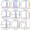 |
Fig. 1. Water maser transitions detected in our sample (Table A.1). Source names and maser transitions are indicated to the right of each panel. Velocities are given in the observed frame. The observed spectra are displayed in black, and single or multiple Gaussian fits are overplotted as colored, semitransparent solid lines. The total fitted emission is shown as a dashed red line. Vertical dashed red lines indicate the systemic velocities of the sources, as listed in Table A.1. For a few panels, the ordinate axis is limited between 20 and 150 Jy to better highlight weaker features. Shaded blue regions indicate the full velocity range of the maser emission, defined as the interval where the fitted model exceeds 3σ above the baseline noise. Horizontal dashed black lines mark the 1 and 3σ noise levels, estimated over the shown velocity range excluding the shaded regions. The bottom-right panel combines all IRAS 16293–2422 submillimeter transitions with a flux limit of 70 Jy to highlight weak spectral features. |
Five sources in the sample exhibit emission from the 31, 3 − 22, 0 transition at 183 GHz, as summarized in Table 1. The 321 GHz transition is detected in only two sources: IRAS 16293–2422 and Serpens FIRS 1. The 325 GHz maser line is detected solely in IRAS 16293–2422, where it exhibits a peak flux density of 497.4 Jy. The corresponding spectral profiles are displayed in Figure 1. With the exception of the 51, 5 − 42, 2 emission in IRAS 16293–2422 (Menten et al. 1990) and the 31, 3 − 22, 0 line in Serpens FIRS 1 (van Kempen et al. 2009), all other detections presented here are reported for the first time.
3.2. Millimeter transitions at 183, 321, and 325 GHz
The measured velocities and flux densities of individual maser components, obtained via multi-Gaussian fitting to the spectral line profiles, are presented in Table A.2. Among the three observed millimeter transitions, the 183 GHz line is the most frequently detected, appearing in all five sources with two to four distinct velocity components each. Peak flux densities span a wide range, from a few janskys up to over 200 Jy. The most prominent detections are toward IRAS 16293–2422 and Serpens FIRS 1. Remarkably, IRAS 16293–2422 is the only source among the 18 observed that exhibits emission from both the 102, 9 − 93, 6 and 51, 5 − 42, 2 H2O maser transitions at 321 and 325 GHz, respectively. The 325 GHz transition shows the highest peak intensity, reaching approximately 497 Jy. Serpens FIRS 1 also shows a detection of the 102, 9 − 93, 6 maser line, which has an upper-state energy of Eup = 1861 K, possibly indicative of stronger shocks or elevated excitation conditions in these two sources relative to the rest of the sample.
In terms of velocity structure, the 183 and 325 GHz components are generally found within ∼5–10 km s−1 of the systemic velocities of their respective sources, though broader deviations are also observed. For example, a 183 GHz component in YLW16A is found at −16.0 km s−1, substantially blueshifted relative to the systemic velocity of 3.6 km s−1. The 321 GHz transition in Serpens FIRS 1 displays primarily redshifted components, reaching up to ∼16 km s−1, while its 183 GHz component is blueshifted relative to the systemic value of 8.0 km s−1.
Overall, the velocity spreads of these maser lines typically range from 10 to 20 km s−1, with a limited number of discrete components per source.
3.3. Comparison of millimeter and centimeter emission
The properties of the 22 GHz maser emission, shown in the final two columns of Table A.2, excluding the reference column, are compiled from previous studies conducted at different epochs and resolutions. Specifically, we adopted data from CARMA 7 (Ortiz-León et al. 2021), Serpens FIRS 1 (Furuya et al. 2003; Bae et al. 2011), L1641N MM1/3 (Bae et al. 2011; Kang et al. 2013), YLW16A (Furuya et al. 2003; Sunada et al. 2007), and IRAS 16293–2422 (Furuya et al. 2003; Sunada et al. 2007). When multiple nearby velocity components are reported, we binned them in 0.5 km s−1 intervals and computed the average velocity. For sources observed across multiple epochs or studies, we adopted the average peak flux density.
A few comparative trends can be noted between the millimeter and centimeter water maser emission. The 22 GHz masers consistently exhibit a larger number of velocity components than any of the millimeter transitions. For instance, IRAS 16293–2422 shows at least nine distinct components at 22 GHz, in contrast to two to four components typically observed at 183, 321, or 325 GHz. Flux densities at 22 GHz are comparable to or exceed those of the brightest millimeter masers. While the 325 GHz line in IRAS 16293–2422 reaches nearly 500 Jy, the 22 GHz maser line shows similarly high peak fluxes across several sources, including 366 Jy in YLW16A.
In terms of velocity coverage, the 22 GHz masers generally span a broader range than their millimeter counterparts. For example, in YLW16A, 22 GHz components extend from −15.2 to +16.3 km s−1, whereas millimeter transitions in the same source exhibit a narrower spread centered closer to the systemic velocity. There are several instances where velocity components from the millimeter and centimeter lines coincide within a few km s−1. However, many features appear in only one frequency regime, suggesting that these transitions trace physically distinct masing regions.
A final caveat warrants emphasis: this comparison is constrained by the non-simultaneity of the observations, as maser emission is known to exhibit significant time variability. Moreover, the identification of velocity-coincident components does not imply spatial coincidence; confirming physical associations among different maser transitions requires spatially resolved, multifrequency observations conducted contemporaneously.
4. Discussion
4.1. Centimeter and millimeter H2O maser lines as probes of star formation
The 22 GHz H2O maser is a well-established tracer of shocked gas at the interface between protostellar jets and the surrounding medium, widely used to probe outflows on scales of tens to hundreds of astronomical units (AU) (Goddi et al. 2017; Moscadelli et al. 2019).
This work presents a first attempt to detect (sub)millimeter water masers at 183, 321, and 325 GHz in low-mass YSOs. These transitions, known in high-mass SFRs, are predicted to be strongly inverted under conditions similar to the 22 GHz line (nH2 ∼ 107–1010 cm−3, Tkin ∼ 400–3000 K; Gray et al. 2016).
So far, millimeter/submillimeter water masers have been imaged in just two high-mass regions (Orion-KL and Cep A) and one low-mass source (Serpens SMM1). In Orion, the 22, 321, and 325 GHz masers trace the same bipolar outflow, suggesting similar excitation conditions (Niederhofer et al. 2012; Greenhill et al. 2013). In Cep A, however, 321 GHz masers appear to trace hotter inner regions not seen at 22 GHz (Patel et al. 2007).
Our comparison (Section 3.3) finds several millimeter and centimeter maser components overlapping in velocity, but many occur independently. This suggests that the transitions often probe different gas regions with varying physical conditions such as temperature, density, or shock velocity. If co-spatial, multi-line observations allow detailed modeling of gas conditions. If not, they offer a layered view of the circumstellar structure. High-resolution interferometry is essential to distinguish between these cases. In both scenarios, combining centimeter and millimeter H2O maser lines offers powerful diagnostics of shocked gas in star formation–either by constraining physical conditions where lines overlap, or by mapping distinct regions in protostellar environments.
4.2. An evolutionary scenario?
Several studies have proposed that masers trace the early evolutionary stages of YSOs, with different molecular species and transitions appearing at different times (e.g., Ellingsen et al. 2007; Reid 2007; Urquhart 2024). In this context, masers could potentially serve as diagnostics for the protostellar phase.
Methanol masers are traditionally divided into two classes: Class I, collisionally pumped and typically found in outflows about 1 pc from ultra-compact H II regions, and Class II, radiatively pumped and tightly associated with high-mass YSOs (Menten 1991; Billington et al. 2020). Notably, both classes can appear before the onset of detectable continuum emission (Ellingsen et al. 1996; Zeng et al. 2020), implying that they trace early phases of star formation. Class II MMs are also observed along with H2O masers (Codella et al. 2004; Goddi et al. 2011), which are commonly associated with shocks in protostellar jets and outflows. However, establishing a strict evolutionary sequence based on maser species remains observationally challenging (e.g., Voronkov et al. 2014). In high-mass YSOs, OH masers are thought to trace more evolved stages, while Class I MMs (e.g., at 84 and 95 GHz) appear earlier (Yang et al. 2023). Unfortunately, OH masers are absent in low-mass YSOs, limiting their diagnostic power in our context.
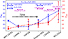 |
Fig. 2. Sources are ordered along the x-axis from youngest to oldest, based on the diffuse dust temperature TDD (see Table 1), which is shown in red and corresponds to the rightmost y-axis. The left y-axis shows the molecular cloud temperature (TMC, in blue), derived from gray-body fits to the SED using the same methodology as for TDD (see Appendix B). Water and MM detections are indicated above each source, with water maser transitions labeled by their frequency in GHz. All temperatures are in kelvin. |
In a recent study, Humire et al. (2024) detected MMs in the J−1 → (J − 1)0-E series for the first time in low-mass YSOs, at J = 7 and 10 (181 and 325 GHz). We refer to these as MMcIs7 and MMcIs10, respectively. If the maser-based evolutionary framework developed proposed for massive YSOs (e.g., Ellingsen et al. 2007) also applies to low-mass objects, then sources exhibiting both 22 GHz water and MMcIs masers should be younger than those with only water masers. To test this scenario, we compared the presence of H2O and CH3OH masers across our sample using an independent age indicator: the diffuse dust temperature (TDD), derived from spectral energy distribution (SED) modeling (see Appendix B and Fig. B.1). We chose TDD over traditional chemical clocks (e.g., S-bearing molecules such as SO or OCS; see Wakelam et al. 2004; Herpin et al. 2009) due to known limitations, which are further expanded upon in Appendix C.
Figure 2 shows the distribution of maser detections as a function of TDD. This plot suggests that water masers tend to appear earlier than MMs in our sample of low-mass YSOs. While this trend appears to contrast with the evolutionary scenario proposed by Ellingsen et al. (2007) for high-mass YSOs, several caveats must be considered. (i) Our analysis is based solely on water and MMs, whereas Ellingsen et al. (2007) also includes OH masers, which are not typically detected in low-mass YSOs. This limits the basis for a direct comparison. (ii) The evolutionary paths of low-mass and high-mass YSOs can differ significantly, implying that maser-based diagnostics might follow different trends. (iii) Our sample is relatively small and lacks the statistical robustness needed for firm conclusions.
With these limitations in mind, we nonetheless explored the possibility that, in low-mass protostars, water masers may indeed emerge earlier than MMs in the course of their evolution. Water masers are more robust under high-velocity shock conditions (v > 10 Km s−1), where methanol molecules are more easily destroyed. H2O, in contrast, can reform efficiently in post-shock gas (Suutarinen et al. 2014), and has higher optical depth in C-type shocks at v > 15 Km s−1 (Nesterenok 2022). These factors may make water masers more likely to appear first, especially during the earliest, most dynamically active phases of low-mass star formation. Additionally, our data enable comparisons across multiple water maser transitions, from the canonical 22 GHz (centimeter) to higher-frequency (millimeter) lines at 183, 321, and 325 GHz. While the 22 GHz line typically traces compact and bright shocked regions, the millimeter transitions can trace more extended structures (e.g., 183 GHz) or warmer gas (e.g., 321 GHz with Eup∼ 1800 K). However, we find no clear trend linking specific H2O transitions to distinct evolutionary phases–possibly due to the overlap of excitation conditions and variability timescales.
In summary, our results suggest that the presence or absence of individual maser transitions cannot serve as a reliable age diagnostic in low-mass YSOs. Water masers, particularly at 22 GHz, appear to be more ubiquitous and may precede MMs in these environments. This challenges simple maser-based evolutionary schemes and highlights the need for multi-tracer, multi-epoch observations to robustly assess YSO evolution.
5. Conclusions
We conducted a survey of H2O masers in 18 low-mass SFRs, all previously known to exhibit emission in the 22 GHz (61, 6 − 52, 3) transition. Our goal was to explore the presence of additional water maser transitions at 183, 321, and 325 GHz, to study their excitation conditions, and to assess their diagnostic potential in relation to evolutionary stages of YSOs.
Our main findings are as follows:
-
We detected the 183 GHz (31, 3 − 22, 0) water maser emission in five sources: IRAS 16293–2422, CARMA 7, Serpens FIRS 1, YLW16A, and L1641N-MM1/3. Among these, IRAS 16293–2422 is the only source that also shows maser emission in both the 321 GHz (102, 9 − 93, 6) and 325 GHz (51, 5 − 42, 2) transitions.
-
By combining these maser data with SED modeling, we used dust temperature as a proxy for evolutionary stage. We find that water masers often appear before or concurrently with Class I MMs, suggesting that masing phenomena using only these two molecules can not be used as a reliable age indicator for low-mass YSOs.
-
We find that several centimeter (from the literature) and millimeter (from this work) maser components occur at similar velocities, but many features are unique to a specific transition. This indicates physically distinct gas regions with different densities, temperatures, or kinematics.
-
While 22 GHz water masers are well-established probes of shocked gas at jet–ambient interfaces, additional detections at 183–325 GHz offer complementary diagnostics. If the maser lines trace the same gas, multifrequency modeling can constrain physical conditions. If not, they provide a layered view of the circumstellar environment at different spatial scales or excitation regimes.
In summary, multifrequency water masers – spanning centimeter to submillimeter wavelengths – offer a promising but complex tool set for probing the early stages of low-mass star formation. High-resolution interferometric imaging of submillimeter lines will be essential to fully exploit their diagnostic potential, clarify the origin of masing regions, and test excitation models.
Efficiency values from http://www.apex-telescope.org/telescope/efficiency/index.php
Acknowledgments
We thank the anonymous referee for their helpful comments, questions, and suggestions on revising the manuscript. P.K.H. gratefully acknowledges the Fundação de Amparo à Pesquisa do Estado de São Paulo (FAPESP) for the support grant 2023/14272-4. C.G. acknowledges financial support by FAPESP under grant 2021/01183-8 and the European Union NextGenerationEU RRF M4C2 1.1 project n. 2022YAPMJH. G.N.O.L. acknowledges the financial support provided by the Instituto Nacional de Astrofísica, Óptica y Electrónica, and Secretaría de Ciencia, Humaninadades, Tecnología e Innovación.
References
- Allen, L. E., Myers, P. C., Di Francesco, J., et al. 2002, ApJ, 566, 993 [NASA ADS] [CrossRef] [Google Scholar]
- Artur de la Villarmois, E., Jørgensen, J. K., Kristensen, L. E., et al. 2019, A&A, 626, A71 [NASA ADS] [CrossRef] [EDP Sciences] [Google Scholar]
- Bae, J.-H., Kim, K.-T., Youn, S.-Y., et al. 2011, ApJS, 196, 21 [NASA ADS] [CrossRef] [Google Scholar]
- Belitsky, V., Lapkin, I., Fredrixon, M., et al. 2018, A&A, 612, A23 [NASA ADS] [CrossRef] [EDP Sciences] [Google Scholar]
- Billington, S. J., Urquhart, J. S., König, C., et al. 2020, MNRAS, 499, 2744 [Google Scholar]
- Cernicharo, J., Thum, C., Hein, H., et al. 1990, A&A, 231, L15 [NASA ADS] [Google Scholar]
- Cernicharo, J., Bachiller, R., & Gonzalez-Alfonso, E. 1996, A&A, 305, L5 [NASA ADS] [Google Scholar]
- Cernicharo, J., Pardo, J. R., González-Alfonso, E., et al. 1999, ApJ, 520, L131 [Google Scholar]
- Chabrier, G. 2003, PASP, 115, 763 [Google Scholar]
- Choi, M., Kang, M., Byun, D.-Y., & Lee, J.-E. 2012, ApJ, 759, 136 [NASA ADS] [CrossRef] [Google Scholar]
- Codella, C., Lorenzani, A., Gallego, A. T., Cesaroni, R., & Moscadelli, L. 2004, A&A, 417, 615 [NASA ADS] [CrossRef] [EDP Sciences] [Google Scholar]
- Crimier, N., Ceccarelli, C., Maret, S., et al. 2010, A&A, 519, A65 [NASA ADS] [CrossRef] [EDP Sciences] [Google Scholar]
- Curiel, S., Rodriguez, L. F., Gomez, J. F., et al. 1996, ApJ, 456, 677 [NASA ADS] [CrossRef] [Google Scholar]
- de Gregorio-Monsalvo, I., Gómez, J. F., Suárez, O., et al. 2006, ApJ, 642, 319 [Google Scholar]
- Drozdovskaya, M. N., van Dishoeck, E. F., Jørgensen, J. K., et al. 2018, MNRAS, 476, 4949 [Google Scholar]
- Dumke, M., & Mac-Auliffe, F. 2010, in Observatory Operations: Strategies, Processes, and Systems III, eds. D. R. Silva, A. B. Peck, & B. T. Soifer, SPIE Conf. Ser., 7737, 77371J [NASA ADS] [CrossRef] [Google Scholar]
- Dzib, S. A., Ortiz-León, G. N., Hernández-Gómez, A., et al. 2018, A&A, 614, A20 [NASA ADS] [CrossRef] [EDP Sciences] [Google Scholar]
- Ellingsen, S. P., Norris, R. P., & McCulloch, P. M. 1996, MNRAS, 279, 101 [Google Scholar]
- Ellingsen, S. P., Voronkov, M. A., Cragg, D. M., et al. 2007, in Astrophysical Masers and their Environments, eds. J. M. Chapman, & W. A. Baan, 242, 213 [NASA ADS] [Google Scholar]
- Enoch, M. L., Glenn, J., Evans, N. J., I., et al. 2007, ApJ, 666, 982 [NASA ADS] [CrossRef] [Google Scholar]
- Froebrich, D. 2005, ApJS, 156, 169 [Google Scholar]
- Furuya, R. S., Kitamura, Y., Wootten, A., Claussen, M. J., & Kawabe, R. 2003, ApJS, 144, 71 [NASA ADS] [CrossRef] [Google Scholar]
- Goddi, C., Moscadelli, L., Alef, W., et al. 2005, A&A, 432, 161 [NASA ADS] [CrossRef] [EDP Sciences] [Google Scholar]
- Goddi, C., Moscadelli, L., Torrelles, J. M., Uscanga, L., & Cesaroni, R. 2006, A&A, 447, L9 [NASA ADS] [CrossRef] [EDP Sciences] [Google Scholar]
- Goddi, C., Moscadelli, L., & Sanna, A. 2011, A&A, 535, L8 [NASA ADS] [CrossRef] [EDP Sciences] [Google Scholar]
- Goddi, C., Surcis, G., Moscadelli, L., et al. 2017, A&A, 597, A43 [NASA ADS] [CrossRef] [EDP Sciences] [Google Scholar]
- Gray, M. D., Baudry, A., Richards, A. M. S., et al. 2016, MNRAS, 456, 374 [NASA ADS] [CrossRef] [Google Scholar]
- Greenhill, L. J., Goddi, C., Chandler, C. J., Matthews, L. D., & Humphreys, E. M. L. 2013, ApJ, 770, L32 [Google Scholar]
- Güsten, R., Nyman, L. Å., Schilke, P., et al. 2006, A&A, 454, L13 [NASA ADS] [CrossRef] [EDP Sciences] [Google Scholar]
- Gutermuth, R. A., Bourke, T. L., Allen, L. E., et al. 2008, ApJ, 673, L151 [NASA ADS] [CrossRef] [Google Scholar]
- Healy, K. R., Hester, J. J., & Claussen, M. J. 2004, ApJ, 610, 835 [Google Scholar]
- Herpin, F., Marseille, M., Wakelam, V., Bontemps, S., & Lis, D. C. 2009, A&A, 504, 853 [NASA ADS] [CrossRef] [EDP Sciences] [Google Scholar]
- Hirota, T., Kim, M. K., & Honma, M. 2012, ApJ, 757, L1 [NASA ADS] [CrossRef] [Google Scholar]
- Hirota, T., Kim, M. K., & Honma, M. 2016, ApJ, 817, 168 [Google Scholar]
- Humire, P. K., Ortiz-León, G. N., Hernández-Gómez, A., et al. 2024, A&A, 688, L1 [NASA ADS] [CrossRef] [EDP Sciences] [Google Scholar]
- Humphreys, E. M. L. 2007, in Astrophysical Masers and their Environments, eds. J. M. Chapman, & W. A. Baan, IAU Symp., 242, 471 [Google Scholar]
- Jacobsen, S. K., Jørgensen, J. K., van der Wiel, M. H. D., et al. 2018, A&A, 612, A72 [NASA ADS] [CrossRef] [EDP Sciences] [Google Scholar]
- Kang, M., Lee, J.-E., Choi, M., et al. 2013, ApJS, 209, 25 [NASA ADS] [CrossRef] [Google Scholar]
- Meledin, D., Lapkin, I., Fredrixon, M., et al. 2022, A&A, 668, A2 [NASA ADS] [CrossRef] [EDP Sciences] [Google Scholar]
- Menten, K. M. 1991, ApJ, 380, L75 [Google Scholar]
- Menten, K. M., Melnick, G. J., Phillips, T. G., & Neufeld, D. A. 1990, ApJ, 363, L27 [NASA ADS] [CrossRef] [Google Scholar]
- Mezger, P. G., Sievers, A. W., Haslam, C. G. T., et al. 1992, A&A, 256, 631 [NASA ADS] [Google Scholar]
- Mizuno, A., Fukui, Y., Iwata, T., Nozawa, S., & Takano, T. 1990, ApJ, 356, 184 [NASA ADS] [CrossRef] [Google Scholar]
- Moscadelli, L., Testi, L., Furuya, R. S., et al. 2006, A&A, 446, 985 [NASA ADS] [CrossRef] [EDP Sciences] [Google Scholar]
- Moscadelli, L., Sánchez-Monge, Á., Goddi, C., et al. 2016, A&A, 585, A71 [NASA ADS] [CrossRef] [EDP Sciences] [Google Scholar]
- Moscadelli, L., Sanna, A., Goddi, C., et al. 2019, A&A, 631, A74 [NASA ADS] [CrossRef] [EDP Sciences] [Google Scholar]
- Moscadelli, L., Sanna, A., Goddi, C., et al. 2020, A&A, 635, A118 [EDP Sciences] [Google Scholar]
- Müller, H. S. P., Schlöder, F., Stutzki, J., & Winnewisser, G. 2005, J. Mol. Struct., 742, 215 [Google Scholar]
- Nakamura, F., Miura, T., Kitamura, Y., et al. 2012, ApJ, 746, 25 [NASA ADS] [CrossRef] [Google Scholar]
- Nesterenok, A. V. 2022, Astron. Lett., 48, 345 [Google Scholar]
- Neufeld, D. A., & Melnick, G. J. 1990, ApJ, 352, L9 [Google Scholar]
- Neufeld, D. A., & Melnick, G. J. 1991, ApJ, 368, 215 [NASA ADS] [CrossRef] [Google Scholar]
- Niederhofer, F., Humphreys, E., Goddi, C., & Greenhill, L. J. 2012, in Cosmic Masers – from OH to H0, eds. R. S. Booth, W. H. T. Vlemmings, & E. M. L. Humphreys, IAU Symp., 287, 184 [Google Scholar]
- Ortiz-León, G. N., Loinard, L., Dzib, S. A., et al. 2018, ApJ, 869, L33 [Google Scholar]
- Ortiz-León, G. N., Plunkett, A. L., Loinard, L., et al. 2021, AJ, 162, 68 [CrossRef] [Google Scholar]
- Patel, N. A., Curiel, S., Zhang, Q., et al. 2007, ApJ, 658, L55 [NASA ADS] [CrossRef] [Google Scholar]
- Peck, A. B., & Impellizzeri, C. M. V. 2018, in Astrophysical Masers: Unlocking the Mysteries of the Universe, eds. A. Tarchi, M. J. Reid, & P. Castangia, IAU Symp., 336, 405 [Google Scholar]
- Pickett, H. M., Poynter, R. L., Cohen, E. A., et al. 1998, J. Quant. Spectr. Rad. Transf., 60, 883 [Google Scholar]
- Planck Collaboration VI. 2020, A&A, 641, A6 [NASA ADS] [CrossRef] [EDP Sciences] [Google Scholar]
- Plunkett, A. L., Arce, H. G., Mardones, D., et al. 2015, Nature, 527, 70 [NASA ADS] [CrossRef] [Google Scholar]
- Reid, M. J. 2007, in Astrophysical Masers and their Environments, eds. J. M. Chapman, & W. A. Baan, 242, 522 [Google Scholar]
- Ronconi, T., Lapi, A., Torsello, M., et al. 2024, A&A, 685, A161 [NASA ADS] [CrossRef] [EDP Sciences] [Google Scholar]
- Sadavoy, S. I., Stephens, I. W., Myers, P. C., et al. 2019, ApJS, 245, 2 [Google Scholar]
- Santos, J. C., Enrique-Romero, J., Lamberts, T., Linnartz, H., & Chuang, K.-J. 2024, ACS Earth Space Chem., 8, 1646 [NASA ADS] [CrossRef] [Google Scholar]
- Slavicinska, K., Boogert, A. C. A., Tychoniec, Ł., et al. 2025, A&A, 693, A146 [NASA ADS] [CrossRef] [EDP Sciences] [Google Scholar]
- Sunada, K., Nakazato, T., Ikeda, N., et al. 2007, PASJ, 59, 1185 [NASA ADS] [Google Scholar]
- Suutarinen, A. N., Kristensen, L. E., Mottram, J. C., Fraser, H. J., & van Dishoeck, E. F. 2014, MNRAS, 440, 1844 [Google Scholar]
- Urquhart, J. S. 2024, in Cosmic Masers: Proper Motion Toward the Next-Generation Large Projects, eds. T. Hirota, H. Imai, K. Menten, & Y. Pihlström, IAU Symp., 380, 135 [Google Scholar]
- van Kempen, T. A., Wilner, D., & Gurwell, M. 2009, ApJ, 706, L22 [Google Scholar]
- van Terwisga, S. E., & Hacar, A. 2023, A&A, 673, L2 [CrossRef] [EDP Sciences] [Google Scholar]
- Vastel, C., Bottinelli, S., Caux, E., Glorian, J. M., & Boiziot, M. 2015, SF2A-2015: Proceedings of the Annual meeting of the French Society of Astronomy and Astrophysics, 313 [Google Scholar]
- Volvach, A. E., Volvach, L. N., & Larionov, M. G. 2022, AJ, 164, 66 [NASA ADS] [CrossRef] [Google Scholar]
- Volvach, A. E., Volvach, L. N., & Larionov, M. G. 2023, A&A, 672, A182 [NASA ADS] [CrossRef] [EDP Sciences] [Google Scholar]
- Voronkov, M. A., Caswell, J. L., Ellingsen, S. P., Green, J. A., & Breen, S. L. 2014, MNRAS, 439, 2584 [NASA ADS] [CrossRef] [Google Scholar]
- Wakelam, V., Caselli, P., Ceccarelli, C., Herbst, E., & Castets, A. 2004, A&A, 422, 159 [NASA ADS] [CrossRef] [EDP Sciences] [Google Scholar]
- Wang, Y. X., Zhang, J. S., Yu, H. Z., et al. 2023, ApJS, 264, 48 [NASA ADS] [CrossRef] [Google Scholar]
- Wilking, B. A., & Claussen, M. J. 1987, ApJ, 320, L133 [Google Scholar]
- Wilking, B. A., Claussen, M. J., Benson, P. J., et al. 1994, ApJ, 431, L119 [Google Scholar]
- Yang, W., Gong, Y., Menten, K. M., et al. 2023, A&A, 675, A112 [NASA ADS] [CrossRef] [EDP Sciences] [Google Scholar]
- Zeng, S., Zhang, Q., Jiménez-Serra, I., et al. 2020, MNRAS, 497, 4896 [NASA ADS] [CrossRef] [Google Scholar]
Appendix A: Individual sources
The present sample consists of Galactic low-mass Class 0-Class I YSOs for which water maser emission at 22 GHz was reported. As a summarized description for several of the sources studied here was presented previously by Humire et al. (2024), we briefly describe water-maser related information only. The exception is YLW16A, for which we provide more detailed information, as it was not covered in depth in our previous work due to the absence of CH3OH maser emission.
NGC 2024 FIR 5/6 is located in the Orion B region, this SFR presents seven compact dust condensations, FIR 1–7, as resolved by Mezger et al. (1992). Among these condensations, FIR 5 and 6 have been suggested to be Class 0 sources were water maser emission at 22 GHz emerges, although their exact emitting source among these two is not fully defined (Furuya et al. 2003, and references therein). However, later studies focusing on the SED of some sub-clumps in NGC 2024 FIR 6 find that one of these highly resolved sources corresponds to a hyper-compact H II region (Choi et al. 2012). As FIR 6 and 5 are separated by about 10″, less than our APEX beam of 19 2 at 325 GHz, it may well be that this hyper-compact H II region, called FIR 6c, is dominating the SED of NGC 2024 FIR 5 (taken at 20″) at IR wavelengths, leading it to be the oldest in the studied sample.
CARMA 7 is a Class 0 protostar, it is the strongest radio source of the Serpens South protostellar cluster. It presents a bipolar and collimated outflow that extends ∼0.16 pc north-south (PA∼4° east of north) in CO emission (Plunkett et al. 2015). The outflow component, as seen by 12COJ = 2–1, exhibits multiple knots with velocities exceeding 10 km s−1 and reaching up to 22 km s−1. The presence of MMs is therefore likely associated with material moving at 5-10 km s−1 away from the source (and projected to ∼0.7 km s−1 from the local standard of rest velocity of the system, as shown in Table 1 of Humire et al. (2024)), observed in about eight knots, namely, before dissociation (see below) (Plunkett et al. 2015). Recently, Ortiz-León et al. (2021) reported water maser emission at 22 GHz in this source.
L1641N(orth) MM1/3 is a dark cloud in the Orion A region ∼7.2 pc south of the Orion Nebula Cluster, hosts the oldest stellar population in L1641 (van Terwisga & Hacar 2023). Cloud-cloud collisions and protocluster winds, inferred from 12CO observations, may explain the CO shells centered at L1641N (Nakamura et al. 2012). Water (22 GHz) maser emission have been encountered in this source (Kang et al. 2013). Its protostar classification lies between Class 0 and I (Froebrich 2005).
Serpens FIRS 1 is a Class 0 protostar located in the main core of the Serpens Molecular Cloud at a distance of 436±9 pc (Ortiz-León et al. 2018). Also known as Serpens SMM 1, this protostar is associated with a bipolar radio jet (e.g., Curiel et al. 1996). It is the most embedded, massive, and luminous YSO in the Serpens dark cloud (Enoch et al. 2007) with a bolometric luminosity of 91 L⊙ (Bae et al. 2011), after correcting for the abovementioned distance. High angular resolution observations at 0 6 revealed a second YSO indicating a binary configuration for this system (Choi et al. 2012). Comparison between single-dish (Furuya et al. 2003) and interferometric observations reveal variable H2O maser emission in this source (Moscadelli et al. 2006).
Sources observed in our water maser survey.
IRAS 16293–2422 is a well-studied Class 0 protostellar system (e.g., Froebrich 2005) known for its strong water maser activity. Located in the Lynds 1689N region of the ρ Ophiuchus cloud at a distance of 141 pc (Dzib et al. 2018), this hierarchical multiple system consists of two main components, IRAS 16293–2422A and IRAS 16293–2422B, surrounded by an extended envelope of ∼8000 AU (Crimier et al. 2010; Jacobsen et al. 2018). IRAS 16293–2422A is divided into two compact sub-sources, A1 and A2.
The distance to this source (141 pc; Dzib et al. 2018) was determined using astrometry of H2O masers observed at 22 GHz with the Very Long Baseline Array. These masers are associated with outflows powered by this system, which, when compact, can reach maximum shifts of 12–16 km s−1, as seen in CO J = 1–0, with respect to the velocity of the system (Mizuno et al. 1990). Interestingly, IRAS 16293–2422 has been routinely monitored over several decades, revealing multiple H2O super flares. This phenomenon has been linked to increased activity in the binary system A. Additionally, variability in H2O masers on timescales of months has been reported by Volvach et al. (2022). The preferentially origin of long-term H2O masers is suggested to be the protoplanetary disk of the A1 compact source (Volvach et al. 2023).
Detected water maser components per source and transition.
YLW16A, also known as IRS 44, has been proposed to be a protobinary system (Allen et al. 2002), although without a clear determination in the submillimeter regime, where Artur de la Villarmois et al. (2019) found accreted shocked gas (up to ∼10 km s−1 with respect to the source’s velocity, as seen in SO2 184, 14 → 183, 15 transition) and a disk-like structure, inferred from SO2 and H13CO+ species, respectively. This latter molecule provides, through position-velocity diagrams, a stellar mass of 1.2±0.1 M⊙. The same authors also provide a couple of reasons why CH3OH is not detected, even when SO and SO2 do. One explanation is that methanol requires a large number density in the pre-shock gas to be released, which is not currently reached by the system. The second possibility is that methanol is released but later destroyed by dissociation at velocities larger than 10 km s−1, as this molecule is expected to survive at moderate velocities, between 3 and 10 km s−1 (Suutarinen et al. 2014). That limitation could also explain the lack of MMs in this source (see Fig. 2).
This source has been classified as a Class I YSO by Sadavoy et al. (2019) based on outflow detection, evidence of a dusty envelope or core, and its bolometric temperature. Additionally, water maser emission at 22 GHz has been reported with high variability, sometimes absent at certain epochs, at velocities between -15 and -10 km s−1 relative to the source’s velocity system Wilking & Claussen (1987), Furuya et al. (2003).
Appendix B: SED modeling and data acquisition
We performed the SED fitting of our six masing sources (see Table 1) using GalaPy (Ronconi et al. 2024), an open-source tool developed in Python/C++ that covers wavelengths from X-ray to radio frequencies. GalaPy assumes a Chabrier initial mass function (Chabrier 2003) and a Λ cold dark matter cosmological model with standard parameters (Planck Collaboration VI 2020).
GalaPy allows for the selection of different star formation history (SFH) models. In this study, we employed the in situ model, which has proven effective in predicting emission in galaxies of various types and epochs (Ronconi et al. 2024). This model enables the evolution of gas, dust, and metallicity to be tracked consistently with star formation evolution, ensuring coherence among derived physical parameters.
Regarding dust, GalaPy implements a two-component model that avoids assuming a fixed attenuation curve, deriving it instead from structural parameters. These two components represent (i) the molecular cloud (MC) phase associated with young stellar populations and (ii) a diffuse medium further attenuating stellar emission. Both contribute to IR emission through two separate modified gray bodies.
Among the various free parameters of this dust model, we fixed certain known values and ranges to ensure physically meaningful results and enhance computational efficiency. Specifically, we set the total number of MCs to NMC = 1, assuming an isolated MC, and constrained their dusty and molecular radii to a typical range of 10–100 pc. A complete list of initial conditions for our SED models is given in Table B.1 while the resulting diffuse dust (TDD) and MC (TMC) temperatures are provided in Table B.2. Other SED modeling results such as MC ages, SFRs, and metallicities are not described, as they are highly dependent on extraction apertures and photometry at optical and radio regimes, which is beyond the scope of this work.
GalaPy input parameter values or ranges common to the six masing sources studied in this work. The terms “log” and “lin” next to the ranges indicate logarithmic (log10) and linear values, respectively.
For a comprehensive list of all GalaPy parameters beyond those considered in this work, which is restricted to the in situ model, we refer the reader to Table B.3 in Ronconi et al. (2024) and its online documentation2.
GalaPy’s SED-fitting results for each source.
The photometric measurements for the six masing sources were obtained from the VizieR photometry viewer3, setting a conservative aperture radius of 20″ to better match our lower angular resolution of 34″, corresponding to the APEX half-power beam width at 181.310 GHz. Repeated observations were discarded leaving the highest in flux only. As we are interested in the dust temperature, quantity that depends on the FIR peak, we also deleted highly variable optical and radio measurements, while in the mid-IR we kept dispersed observations as the model naturally fit the largest values, as can be most noticeable seen for CARMA 7, L1641N MM1/3, and Serpens FIRS 1 in Fig. B.1.
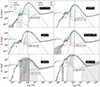 |
Fig. B.1. SED models obtained with the GalaPy software for the sources studied in this work (see Appendix A). Points correspond to the photometric measurements obtained from the VizieR photometry viewer (see Appendix B), while solid lines correspond to the unattenuated stellar emission (green), molecular cloud component (MC, purple), stellar emission considering extinction (extinct, red), and diffuse dust (DD, yellow). |
Appendix C: Sulfur-bearing molecules as an age estimator
As an age estimator, we avoided using sulfur-bearing molecules such as OCS, SO, and SO2, which have been proposed as potential chemical clocks in previous studies (e.g., Wakelam et al. (2004), Herpin et al. (2009)). This decision is based on two key reasons:
-
Limited observational constraints: Our measured line ratios (SOJ = 78–67/OCSJ = 16–15 ∼ 10–70 and SO2J = 91, 9–80, 8/OCS ∼ 1–8; not shown) show orders-of-magnitude differences compared to column density ratios from high-resolution ALMA observations of IRAS 16293-2422 (Drozdovskaya et al. 2018), where SO/OCS = 0.2% (0.002) and SO2/OCS = 0.5% (0.005) in the compact component, and SO/OCS = 63% (0.63) and SO2/OCS = 9% (0.09) in the more extended region. These discrepancies suggest our line ratios cannot be directly interpreted as column density ratios likely due to opacity effects mainly on the OCS line.
-
Uncertainties in sulfur chemistry: The underlying chemical evolution of sulfur-bearing molecules remains poorly understood. Key issues include (i) the unknown reservoir of sulfur in interstellar ices (whether H2S, atomic S, or other compounds such as NH4SH; Slavicinska et al. 2025 are predominant), (ii) the sensitivity of sulfur chemistry to grain-surface processes and thermal history prior to protostar formation, and (iii) the strong dependence of observed abundances on desorption temperatures (e.g., SO2 vs. OCS). Recent studies (Santos et al. 2024) also highlight inconsistencies in using these species as evolutionary tracers, as their abundances may reflect local conditions (e.g., protostellar temperature) rather than source age.
All Tables
GalaPy input parameter values or ranges common to the six masing sources studied in this work. The terms “log” and “lin” next to the ranges indicate logarithmic (log10) and linear values, respectively.
All Figures
|
Fig. 1. Water maser transitions detected in our sample (Table A.1). Source names and maser transitions are indicated to the right of each panel. Velocities are given in the observed frame. The observed spectra are displayed in black, and single or multiple Gaussian fits are overplotted as colored, semitransparent solid lines. The total fitted emission is shown as a dashed red line. Vertical dashed red lines indicate the systemic velocities of the sources, as listed in Table A.1. For a few panels, the ordinate axis is limited between 20 and 150 Jy to better highlight weaker features. Shaded blue regions indicate the full velocity range of the maser emission, defined as the interval where the fitted model exceeds 3σ above the baseline noise. Horizontal dashed black lines mark the 1 and 3σ noise levels, estimated over the shown velocity range excluding the shaded regions. The bottom-right panel combines all IRAS 16293–2422 submillimeter transitions with a flux limit of 70 Jy to highlight weak spectral features. |
| In the text | |
|
Fig. 2. Sources are ordered along the x-axis from youngest to oldest, based on the diffuse dust temperature TDD (see Table 1), which is shown in red and corresponds to the rightmost y-axis. The left y-axis shows the molecular cloud temperature (TMC, in blue), derived from gray-body fits to the SED using the same methodology as for TDD (see Appendix B). Water and MM detections are indicated above each source, with water maser transitions labeled by their frequency in GHz. All temperatures are in kelvin. |
| In the text | |
|
Fig. B.1. SED models obtained with the GalaPy software for the sources studied in this work (see Appendix A). Points correspond to the photometric measurements obtained from the VizieR photometry viewer (see Appendix B), while solid lines correspond to the unattenuated stellar emission (green), molecular cloud component (MC, purple), stellar emission considering extinction (extinct, red), and diffuse dust (DD, yellow). |
| In the text | |
Current usage metrics show cumulative count of Article Views (full-text article views including HTML views, PDF and ePub downloads, according to the available data) and Abstracts Views on Vision4Press platform.
Data correspond to usage on the plateform after 2015. The current usage metrics is available 48-96 hours after online publication and is updated daily on week days.
Initial download of the metrics may take a while.