| Issue |
A&A
Volume 701, September 2025
|
|
|---|---|---|
| Article Number | A146 | |
| Number of page(s) | 7 | |
| Section | Interstellar and circumstellar matter | |
| DOI | https://doi.org/10.1051/0004-6361/202556539 | |
| Published online | 10 September 2025 | |
Estimating the infrared band strengths of amorphous interstellar ice analogues using density functional theory
1
Centro de Astrobiología (CSIC-INTA),
Ctra. de Ajalvir, km 4,
Torrejón de Ardoz,
28850
Madrid,
Spain
2
Departamento de Química Física, Facultad de C. Químicas,
Universidad Complutense, and Unidad Asociada Physical Chemistry UCM-CSIC,
28040
Madrid,
Spain
★ Corresponding author: This email address is being protected from spambots. You need JavaScript enabled to view it.
Received:
22
July
2025
Accepted:
5
August
2025
Abstract
Context. Infrared band strengths are needed to obtain the column density of ice mantle molecular components observed towards cold interstellar and circumstellar environments. The values for these ices are often outdated or unavailable.
Aims. Using density functional theory, we aim to provide a general method for the prediction and confirmation of band strengths for any amorphous ice.
Methods. Amorphous ices were created using randomised initial positions of molecules in a cubical simulation box with periodic boundary conditions to simulate an infinite amorphous solid. Temperature was controlled using molecular dynamics with a thermostat and maintaining a constant volume. Infrared spectra were subsequently generated according to density functional perturbation theory. Results. Estimations for band strengths are presented for ices of astrophysical interest, including water, carbon dioxide, carbon monoxide, methane, ammonia, and methanol.
Conclusions. The newly calculated band strengths are in good agreement with previous values obtained through experimental measurements. This novel method can be applied in general to any amorphous ice, with especially good accuracy for bending vibrational modes. The method can also be applied to ices of unknown band strengths, including unstable species under Earth conditions, and to mixed or layered ices that contain more than one species.
Key words: methods: numerical / techniques: spectroscopic / ISM: abundances / ISM: lines and bands / infrared: ISM
© The Authors 2025
 Open Access article, published by EDP Sciences, under the terms of the Creative Commons Attribution License (https://creativecommons.org/licenses/by/4.0), which permits unrestricted use, distribution, and reproduction in any medium, provided the original work is properly cited.
This article is published in open access under the Subscribe to Open model. This email address is being protected from spambots. You need JavaScript enabled to view it. to support open access publication.
1 Introduction
Infrared (IR) spectroscopy is used to analyse the composition and structure of ices in the interstellar medium (ISM; Tielens & Whittet 1997). IR absorption occurs at specific frequencies for each molecule, known as vibration bands, each of which has a specific sensibility or band strength. Previous knowledge of the band strength is necessary to interpret the IR spectra, allowing observers to determine the composition and relative abundances of species within the ice. Band strengths for all molecular vibrations of the most common ices observed in the ISM were determined experimentally decades ago (e.g. Hagen et al. 1981; d’Hendecourt & Allamandola 1986). They have been updated multiple times following technological advances (see e.g. Luna et al. 2012; Satorre et al. 2017). However, interstellar ice analogues grown via vapour deposition are inherently porous; this complicates the measurement of their density, which is necessary for determining the band strength. Uncertainties about ice densities, and hence band strengths, remain to this day, even in the case of the most studied molecules and ices, such as H2O, CO2, and NH3 (Mastrapa et al. 2009; Bouilloud et al. 2015). In the case of water ice, Hagen et al. (1981) is still used as a reference for the IR band strength, but this work reports a constant value of 2 × 10⁻¹⁶ cm molecule−1 for all the ice temperatures. In a recently published work, we reported the IR O–H stretching band strength of water ice at different temperatures (Escribano et al. 2025), introducing a notable correction with respect to previous values. Due to the difficulty of measuring band strengths and the discrepancies generated by even minor differences in experimental setups, it is worth resorting to some of the most reliable methods of computational chemistry as an alternative approach to predicting or confirming experimental measurements of band strengths.
Infrared spectroscopy measures the interaction of electromagnetic radiation with the dipole moment of molecules. Therefore, in order to simulate this interaction accurately, it is necessary to apply a level of theory that includes electronic structure. Density functional theory (DFT; Hohenberg & Kohn 1964; Kohn & Sham 1965) is a computational method that uses quantum mechanics to model the electronic interaction between atoms, including molecular polarisation, and is capable of generating simulated IR spectra with great accuracy in both the vibrational band frequencies and absorption intensities (Refson et al. 2006). Such simulations have recently been used to predict previously unknown band strengths of single molecules (Taillard et al. 2025) but with a relatively low estimated accuracy (at least an order of magnitude). More accurate and realistic estimations would require simulating amorphous solids made of many molecules, which is computationally unfeasible. Small clusters of molecules combined with statistical mechanics have been used to simulate ultraviolet spectra of amorphous ices of astrophysical relevance (Wallace & Fortenberry 2021, 2022). This method yields more realistic results but is still limited by the small size of the clusters and, thus, cannot reproduce the effects of density and porosity. The different levels of theory available in DFT methods were recently benchmarked for their application to amorphous ices by Woon (2024).
In this work, we present a novel general model for the simulation of amorphous ices with any chosen density and deposition temperature, allowing the prediction of band strengths with a similar level of precision and reproducibility as the experimental values available in the bibliography. The method uses periodic boundary conditions to simulate an infinite amorphous solid while being computational inexpensive, using very few molecules in the simulation box. The method is particularly useful for those ices whose band strengths have never been measured experimentally or those that have been measured erroneously in the past, as well as for mixtures of ices with more than one species. Regarding the band strengths in ice mixtures, only a few publications are available (d’Hendecourt & Allamandola 1986; Hudgins et al. 1993).
2 Calculations and mathematical derivations
All molecular dynamics (MD) and DFT simulations were performed using the open-source plane-wave pseudo-potential method CASTEP (Clark et al. 2005). Amorphous ices were first constructed by assigning randomised initial positions for N molecules in a cubic simulation box with volume V and periodic boundary conditions to emulate an infinite solid. The density (ρ) of the ice is the main parameter of the simulation and is defined as N times the molecular mass (mmolec) divided by the volume of the simulation box. To simulate temperature, we then integrated an MD trajectory of 100 ps with a timestep of 1 fs in the NVT ensemble using a Nose-Hoover thermostat (Martyna et al. 1992). Following the MD trajectory, we applied a DFT geometry optimisation using the Perdew–Burke–Ernzerhof functional of the generalised gradient approximation (Troullier & Martins 1991; Perdew et al. 1996).
It is well known that the application of DFT methods to molecular aggregates requires the explicit inclusion of a correction to take the important dispersive effects into account. In our case, long-range dispersion correction was implemented using the Grimme D2 method (Grimme 2006). We are aware that more accurate versions of Grimme corrections exist, such as the recent D4 method (Caldeweyher et al. 2017), which perform very well in complex systems that include transition metals, coordination compounds, or ions. Unfortunately, the algorithm is not implemented in the CASTEP software. However, it must be considered that we are dealing here with small, neutral, moderately polar (or non-polar) molecules that comprise only atoms from the two first rows of the periodic table. This fact together with the good results we obtained in previous calculations using a similar methodology in akin systems (Escribano et al. 2019) seems to justify our choice. For these calculations, basis functions were taken from the literature (Corsetti et al. 2013), the energy convergence parameter was set to 10−6 eV/Å, and the cutoff was set to 925 eV.
The simulated IR spectrum was computed using CASTEP’s linear response algorithm, which implements density functional perturbation theory (Refson et al. 2006). This method provides discrete IR absorption peaks with specific frequencies and intensities corresponding to molecular IR vibrational bands. A continuous absorption band, to be compared with experimental spectra, was artificially recreated through the addition of Lorentzian distributions centred at each discretely predicted vibration (see Fig. 1). The number of absorption peaks per band increases with the number of molecules (N) in the simulation box, resulting in a more realistic reconstruction of the continuous experimental band. The intensity of these discrete absorptions was then summed to obtain the total absorption for that vibration mode, which was finally divided by N to obtain the band strength in cm molecule−1.
The statistical representation of amorphous ices improves with increasing number of molecules (N) in the simulations box. However, the computational cost of DFT methods scales proportionally to N3, so it is advisable to keep the N as small as possible while maintaining consistent values for the band strength. In Fig. 2, we observe how the calculated band strength converges for N≥8, so all results presented in this work have been computed with N=8.
We measured the accuracy of our method by comparing our simulated band strengths to experimental values, which are commonly measured using an IR spectrometer combined with laser interferometry (González Díaz et al. 2022). The band strength (A) is defined as
 (1)
(1)
where mmolec is the molecular mass, Aint is the integrated absorbance of the IR band, NA is the Avogadro constant, d is the thickness of the ice layer measured via interferometry, and ρ(T) is the density of the ice at temperature T, which must be previously known. It is worth noting that not all band strengths vary significantly with temperature, as this effect is related to the composition and structural changes of the ice (e.g. Mastrapa et al. 2009; Carrascosa et al. 2023).
The main limitation of the DFT method, which is shared by the experimental determination of the IR band strengths, is that previous knowledge of the density is not always available or is not accurate. Measuring the density of a vapour-deposited amorphous ice requires a different and complex experimental setup (Domingo-Beltrán et al. 2015). Additionally, the conditions during ice growth will affect the internal structure of the ice, including crystallinity and porosity, heavily influencing the density measurement.
It is well known that many band strengths measured in this way are based on incorrect densities; this issue is discussed in Escribano et al. (2025). If a density is unknown, it is often assumed to be 1 g cm−3 (Hudgins et al. 1993). When a better, updated measurement of the density becomes available, an approximate correction can be immediately applied as
 (2)
(2)
where A′ is the corrected band strength, A is the previously published band strength, ρ is the ‘wrong’ density used in the calculation of A, and ρ′ is the updated value, more accurate density (Bouilloud et al. 2015).
In the following section, we present a comparison for the most common ices of astrophysical interest, including simulated IR results and experimental examples of ices grown in our ultra-high-vacuum (UHV) chamber ISAC. This experimental setup is described in detail in Muñoz Caro et al. (2010).
 |
Fig. 1 Example of a simulated IR spectrum for a system of eight water molecules. Blue lines are calculated vibrations with discrete frequency and absorption intensity. The black line is the addition of Lorentzian curves centred at each vibration with a full width at half maximum of 25 cm−1. |
 |
Fig. 2 Example of a calculated band strength for a water ice system at 50 K with an increasing number of molecules (blue) along with the associated computational time (orange). |
3 Results
The results of the simulations are presented in Fig. 3, where we compare the simulated spectra with experimental examples deposited at 10 K. Source data for both the experimental and simulated spectra are provided as supplemental material for reproducibility. The resulting band strength values are presented in Table 1, where the calculated values are compared to some of the most recent experimental measurements. In the following subsections we detail each ice separately.
3.1 Water (H2O)
Water is the most studied amorphous ice and has been detected in IR observations of dense interstellar clouds and protoplan-etary disks (Gibb et al. 2004), as well as on the surface of comets (Mumma & Charnley 2011), moons, and planets (Baragiola 2003).
The recent deployment of the James Webb Space Telescope (JWST) has provided unprecedented spectral resolution for the analysis of such ices (McClure et al. 2023). The band strengths that are commonly used in the interpretation of these IR spectra were provided by Hagen et al. (1981); however, they are known to be erroneous as they were calculated using a density value of 0.94 g cm−3 (Narten et al. 1976), which assumes no porosity, as well as ignoring any variation with temperature.
In our previous work (Escribano et al. 2025) we experimentally measured the O-H stretching band strength of water ice for all temperatures using updated density values provided by Dohnálek et al. (2003). The resulting values are presented in Fig. 4 (orange squares); they vary strongly with temperature, and a correction of at least 40% with respect to Hagen et al. (1981, green line in Fig. 4) is needed. In the current work, we used the same densities to generate simulated amorphous water ices. The resulting calculated band strengths are represented as orange circles in Fig. 4. If we simulated ice using the same density as Hagen et al. (1981), the resulting band strength would not meet their experimental results, meaning that their assumption for density was incorrect (see the green circles in Fig. 4). This is expected and has been discussed in previous works (Mastrapa et al. 2009; Bouilloud et al. 2015).
In Fig. 4, we also show experimental values for ice deposited at 10 K and then slowly warmed (blue line). The DFT-simulated values appear to be closer to this experiment’s results than the individual experiments deposited at different temperatures. A possible explanation for this is that our MD trajectory of 100 ps is long enough to simulate a warm-up experiment, where molecular self-diffusion is non-negligible. This is especially notable at approximately 80 K, when the band strength value decreases for both the experiment and the simulations. This is the estimated onset temperature of crystallisation for amorphous water ice (Olander & Rice 1972).
3.2 Carbon dioxide (CO2)
The IR spectrum for carbon dioxide ice presents two well-defined bands, one each for the asymmetric stretching and the bending vibrations. The simulated IR spectrum manages to reproduce both with good accuracy for the frequency and the absorption intensity (Fig. 3, top middle). It is worth noting that the resulting band strengths are slightly overestimated for the stretching mode compared to the bending mode (see Table 1), a phenomenon that we found in several ices and that we discuss in the next section.
The asymmetric stretching mode for amorphous CO2 is more complex than what can be appreciated in Fig. 3. The shape and spectral frequency of the band is affected by isotopic abundances (Falk 1987), porosity (Gálvez et al. 2008), and interactions with other molecules (Sandford & Allamandola 1990). Recent observations from the JWST of Jupiter’s moon Europa show how abundances and molecular mixtures can be extracted from this band (Villanueva et al. 2023). The accurate representation of this band using DFT simulations has recently been tested in the interpretation of IR spectra from Ganymede and Europa by Schiltz et al. (2024), who used simulations to showcase the effect of porosity on the shape and position of the band.
3.3 Carbon monoxide (CO)
Results for carbon monoxide from experiments and simulations show very good agreement, both for the band position on the spectrum and the absorbance, with a deviation in band strengths of less than 10% (see Table 1 and Fig. 3, top right). It is particularly easy to simulate this ice because the density of CO is well defined and varies only slightly with temperature (Luna et al. 2022).
The slight overestimation of the band strength can be attributed to minor differences in experimental conditions. Our reference density was taken from Bouilloud et al. (2015), who performed experiments at 25 K, while the commonly accepted band strength was measured by Gerakines et al. (1995) at 14 K. At 25 K, the amorphous-crystalline phase transition is already underway (González Díaz et al. 2022). In the crystalline phase, the band can be decomposed into two components, the transversal optical (TO) mode at 2138 cm−1 and the longitudinal optical (LO) mode at 2142 cm−1 (Palumbo 2006). When the IR spectrum is generated with a normal incidence, the IR radiation is only sensitive to the TO mode (González Díaz et al. 2025) and therefore shows a weaker absorption on the spectrum. However, our simulation method is not affected by this limitation and includes absorption equally in both perpendicular directions. This would explain why our band strength is slightly higher, as well as the band position being slightly blueshifted towards the LO mode.
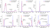 |
Fig. 3 Comparisons between DFT-simulated IR spectra and laboratory experimental spectra. All ice samples shown were deposited at 10 K; simulations were thermalised with MD with a thermostat at 10 K. Minor disagreements in band positions are caused by potential differences in density estimations, which are experimentally uncertain. Simulated spectra are represented as Lorentzian curves with a full width at half maximum of 25 cm−1. Absorbance intensities have been normalised for clarity. Source data for all spectra are provided as supplemental material. |
Band strengths calculated using simulated DFT spectra compared to previously measured experimental values corrected by density ρ′.
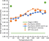 |
Fig. 4 Water ice band strength for the O-H stretching band, comparing experimental and simulation values. The Hagen DFT results (green dots) are based on the density from Narten et al. (1976). The Escribano DFT results (orange dots) are based on densities from Dohnálek et al. (2003). |
3.4 Methane (CH4)
The results of methane ice simulations are in good agreement with experimental values (see Table 1), although they overestimate the stretching mode (ν3) at 3010 cm−1 compared to the bending mode (ν4) at 1302 cm−1. In Fig. 3 (bottom left), we can see a slight divergence in the band positions with respect to the experiment. This is likely caused by a difference in density, which we cannot measure with our experimental setup and can be affected by external factors such as the deposition rate and directionality. The internal structure of the ice and its density are always affected by the mechanism used to inject the depositing gas into the vacuum chamber. Faster deposition rates and oblique angles lead to columnar and dendritic growths (González Díaz et al. 2019), while slower depositions at a perpendicular angle lead to more uniform, denser ice films (e.g. Escribano et al. 2025; Cazaux et al. 2015).
Additionally, we notice that our experimental spectrum has a proportionally higher absorbance for the bending band than observed in other similar experiments (e.g. Hudgins et al. 1993; Bouilloud et al. 2015). This could be explained by the lower deposition rate of our UHV chamber. Condensed methane is a particularly difficult ice because it has one amorphous and two crystalline phases with a phase transition at a very low temperature, approximately 20 K. If the deposition rate is not low enough, the temperature at the ice surface will not be stable and the amorphous and crystalline phases could coexist even below 20 K. Gerakines & Hudson (2015) show that the band strength for the bending mode of a purely amorphous ice could have been previously underestimated by as much as 33% as a consequence. They report a new band strength of 1.04 × 10⁻¹⁷ cm molecule−1 at 10 K, very close to our simulated value.
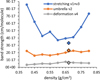 |
Fig. 5 Band strengths for NH3 amorphous ice simulated for a range of densities. Diamonds are experimental values from Sandford & Allamandola (1993) corrected using the updated density from Satorre et al. (2013). |
3.5 Ammonia (NH3)
Ammonia ice is particularly complex. The divergence between simulations and experiments for the stretching band is the worst of all ices, while the discrepancies for the two bending bands (umbrella and deformation) are among the smallest. The band strengths in Table 1 have been corrected with the most recent measurements of density by Satorre et al. (2013), although in that work the authors only reached 13 K and the ammonia density at 10 K is expected to be even lower. However, even with the uncertainty in density, our method still overestimates the sensitivity of the stretching band by a surprising amount, considering how well other bands are predicted by the simulations. To understand why this is the case, we performed simulations of ammonia ice for a range a densities between 0.4 and 0.8 g cm−3. The results are plotted in Fig. 5. We can see that the bending modes vary little with density, while the stretching mode only produces credible results between 0.5 and 0.7 g cm−3 and always above the experimental values (marked with diamonds in Fig. 5). An explanation for this is that the N–H bonds in ammonia are coupling between adjacent molecules, producing an exaggerated vibration that is very sensitive to the intermolecular distance. Meanwhile, the bending modes are defined by intramolecular interactions and are shielded from the effect of changing density.
A similar result was reported by Zanchet et al. (2013). Using both experiments and DFT simulations, they determined a proportionally weaker absorption for the stretching band when N2 molecules are added to the ammonia ice. These molecules acted as a buffer that impedes the coupling of the N–H stretching vibrations between NH3 neighbours, resulting in a very diminished stretching band, while the bending bands were mostly unaffected.
3.6 Methanol (CH3OH)
Methanol ice has a complex stretching mode set that includes several O-H and C-H vibrations, which are often integrated together in the IR spectrum between 2700 and 3600 cm−1. A full description of the complexities of this band can be found in Carrascosa et al. (2023), where the authors obtained an updated value for its band strength using density measurements from Luna et al. (2018b). In Table 1 we see, once again, a very good agreement between simulation and experiment results, with a slight overestimation of this complex stretching band.
The C–O stretching mode was not measured by Carrascosa et al. (2023), but our estimate has an almost exact agreement with the band strength measured by Hudgins et al. (1993) and corrected with the density by Luna et al. (2018b). This vibrational mode is mostly intramolecular and is not affected by the hydrogen bonds that tend to form intermolecular chains in methanol ice (Falk & Whalley 1961).
An alternative measurement of methanol band strengths was provided by Bouilloud et al. (2015), although in that case the density for the crystalline α-phase was employed. The resulting band strengths are very different from ours and those of Hudgins et al. (1993) and d’Hendecourt & Allamandola (1986).
4 Discussion
In general, the results of our novel method for estimating IR band strengths show very good agreement with experimental values for all the ices studied. The accuracy of the method is strongly dependent on the previous knowledge of the ice density, which is not always available or might be erroneous. We have found that applying the density correction proposed by Bouilloud et al. (2015) significantly improves the results. This is not surprising considering that many band strengths in the bibliography were calculated when micro-balances were not available and density measurements were obtained using diffraction experiments, which do not account for the porosity of the ice. Furthermore, when a density was not known, it would be assumed to be 1g cm−3 (Hudgins et al. 1993), introducing errors higher than 50% with respect to modern measurements.
Simulated bending bands are particularly accurate, but the divergence with experiments is always below 25% except in the case of the N–H stretching band of NH3 ice. We have found that hydrogen bonds, and especially N–H bonds, tend to produce a molecular coupling where the vibration is overestimated. This is a limitation of the method that could be remedied by using a more specific functional for the DFT geometry optimisation. Other observed discrepancies can be explained through minor differences or inaccuracies in experimental methods. For example, not all authors deposited their ices at 10 K, with warmer temperatures producing less porosity (Bossa et al. 2015). Different deposition angles also affect the structure of the ice, influencing the measured density and band strength (Dohnálek et al. 2003). Our method only relies on the density parameter, which can be exactly controlled, leading to more reproducible and applicable band strengths.
The sensibility to hydrogen bonds can be used to highlight the different origin of the IR vibrations. Stretching vibrations can lead to a coupling interaction between two or more molecules and are very sensitive to changes in density, sometimes producing synchronisation patterns that lead to separate IR bands (Carrascosa et al. 2023). These modes will have very different band strengths in the gas and solid phases. On the other hand, bending modes are defined by intramolecular forces and are not as strongly affected by changes in density. When available, it is advisable to use these bands for interpreting IR spectra and determining column densities, as their band strength values are considered more reliable.
The sensibility of the stretching modes can also be applied to find realistic ranges of densities. As we report in the case of NH3, our method only produces credible results for the stretching band between 0.5 and 0.7 g cm−3. There is still some uncertainty regarding the density of ammonia ice. Luna et al. (2018a) find a density of 0.67 g cm−3, which is lower than previously thought, but the density is believed to be even lower as the temperature decreases to close to 0 K. Our method can provide lower and upper bounds for ice densities in interstellar conditions, especially when those conditions are difficult or impossible to achieve in the laboratory.
In this work, we focused on pure ices, but in interstellar and cometary ices it is often uncertain whether the different components of the icy phase are mixed or segregated in layers. The general method proposed here can be immediately applied to mixed or layered ices with two or more molecular species, which encompasses most of the ices observed in the ISM. The study of such ices incurs many experimental complications and uncertainties, but in a simulation box the composition and the density of the ice can be defined exactly. In the past, having an estimation for band strengths in mixed ices required broad approximations (see e.g. Schiltz et al. 2024), which can be avoided with DFT simulations.
Even when there is no previous knowledge about the density of the ice, our method can be applied to estimate a range of realistic band strengths if one can approximate a value for the density. This approach has recently been applied to interpret spectra of SO2 ices, which, following ultraviolet irradiation, contained some amount of SO3 ice (Martín-Doménech et al. 2025).
5 Conclusions
We have introduced a novel method for estimating IR band strengths of amorphous ices using DFT, and we have demonstrated its use for the most commonly observed astrophysical ice components. Our main conclusions are as follows:
Band strengths calculated using DFT are in good agreement with those measured experimentally, in most cases with a discrepancy of less than 25%, provided there is accurate knowledge of the ice density. When the density is unknown, our method can provide a range of expected band strengths corresponding to a range of densities. In future work, we expect to be able to provide accurate estimations for both densities and band strengths that will converge to the experimental values;
Many band strengths that are currently in use when interpreting IR observations for estimation of the column density are known to be inaccurate as they are based on erroneous density values. Our method can correct those band strengths, confirming the corrections proposed by Bouilloud et al. (2015), including some of their more dubious corrections, as in the case of water ice. Our method also helps explain some of the discrepancies between studies, as in the case of methanol ice (Hudgins et al. 1993; d’Hendecourt & Allamandola 1986), which was recently significantly corrected by Carrascosa et al. (2023);
We have found that stretching vibrational modes, especially those involving hydrogen, can produce intermolecular couplings that overestimate the IR absorption. This phenomenon is problematic in DFT simulations as well as in experimental measurements when the density value is not accurately known. It is preferable to focus on bending or deformation modes when they are spectroscopically available;
The method can be immediately extended to the simulation of mixed ices composed of several different molecular species. Most observations of astrophysical ices include a mixture of molecules. The experimental study of such mixtures incurs complexities and uncertainties that can be better tackled using DFT simulations, in which densities and relative compositions can be exactly controlled;
Some unstable species that are not commercially available, such as SO, CS, and OCN−, do not have known band strengths. It is unfeasible to measure such values in the laboratory, but they present no additional complexity when using our approach, and the resulting estimation should be as reliable as for any other ice.
Band strengths calculated with our method can confirm previously known values, correct existing errors, or provide a trustworthy first estimation when there is no experimental value available. In a future work we will apply this DFT method to mixed and layered ices that resemble the architecture of interstellar or circumstellar ice mantles but whose IR band strengths are difficult to measure experimentally.
Data availability
The dataset tables for all experimental and simulated IR spectra are available at https://doi.org/10.5281/zenodo.16751748.
Acknowledgements
This research has been funded by the projects PID2020-118974GB-C21, PID2020-118974GB-C22, PID2023-151513NB-C21, and PID2023-151513NB-C22 by the Spanish Ministry of Science and Innovation. B.E. acknowledges the support by grant PTA2020-018247-I from the Spanish Ministry of Science and Innovation/State Agency of Research MCIN/AEI. R.M.-D. was supported by a La Caixa Junior Leader grant under agreement LCF/BQ/PI22/11910030. P.C.G. acknowledges support by grant PID2021-122839NB-IDD by the Spanish Ministry of Science and Innovation.
References
- Baragiola, R. A. 2003, Planet. Space Sci., 51, 953 [NASA ADS] [CrossRef] [Google Scholar]
- Bossa, J.-B., Maté, B., Fransen, C., et al. 2015, ApJ, 814, 47 [NASA ADS] [CrossRef] [Google Scholar]
- Bouilloud, M., Fray, N., Bénilan, Y., et al. 2015, MNRAS, 451, 2145 [Google Scholar]
- Caldeweyher, E., Bannwarth, C., & Grimme, S. 2017, J. Chem. Phys., 147 [Google Scholar]
- Carrascosa, H., Satorre, M. Á., Escribano, B., Martín-Doménech, R., & Muñoz Caro, G. 2023, MNRAS, 525, 2690 [NASA ADS] [CrossRef] [Google Scholar]
- Cazaux, S., Bossa, J.-B., Linnartz, H., & Tielens, A. 2015, A&A, 573, A16 [NASA ADS] [CrossRef] [EDP Sciences] [Google Scholar]
- Clark, S. J., Segall, M. D., Pickard, C. J., et al. 2005, Z. Kristall., 220, 567 [NASA ADS] [Google Scholar]
- Corsetti, F., Fernández-Serra, M., Soler, J. M., & Artacho, E. 2013, J. Phys.: Condens. Matter, 25, 435504 [Google Scholar]
- d’Hendecourt, L., & Allamandola, L. 1986, A&AS, 64, 453 [Google Scholar]
- Dohnálek, Z., Kimmel, G. A., Ayotte, P., Smith, R. S., & Kay, B. D. 2003, J. Chem. Phys., 118, 364 [CrossRef] [Google Scholar]
- Domingo-Beltrán, M., Luna-Molina, R., Ángel Satorre-Aznar, M., Santonja-Moltó, C., & Millán-Verdú, C. 2015, Sensors, 15, 25123 [Google Scholar]
- Escribano, R., Gómez, P. C., Maté, B., Molpeceres, G., & Artacho, E. 2019, Phys. Chem. Chem. Phys., 21, 9433 [Google Scholar]
- Escribano, B., del Burgo Olivares, C., Carrascosa, H., et al. 2025, A&A, 699, A79 [NASA ADS] [CrossRef] [EDP Sciences] [Google Scholar]
- Falk, M. 1987, J. Chem. Pys., 86, 560 [Google Scholar]
- Falk, M., & Whalley, E. 1961, J. Chem. Phys., 34, 1554 [Google Scholar]
- Gálvez, O., Maté, B., Herrero, V. J., & Escribano, R. 2008, Icarus, 197, 599 [CrossRef] [Google Scholar]
- Gerakines, P. A., & Hudson, R. L. 2015, ApJ, 805, L5 [NASA ADS] [CrossRef] [Google Scholar]
- Gerakines, P. A., Schutte, W. A., Greenberg, J. M., & van Dishoeck, E. F. 1995, A&A, 296, 810 [NASA ADS] [Google Scholar]
- Gibb, E., Whittet, D., Boogert, A., & Tielens, A. 2004, ApJS, 151, 35 [NASA ADS] [CrossRef] [Google Scholar]
- González Díaz, C., Carrascosa, H., & Muñoz Caro, G. M. 2025, MNRAS, 538, 1906 [Google Scholar]
- González Díaz, C., Carrascosa de Lucas, H., Aparicio, S., et al. 2019, MNRAS, 486, 5519 [CrossRef] [Google Scholar]
- González Díaz, C., Carrascosa, H., Muñoz Caro, G. M., Satorre, M. Á., & Chen, Y. J. 2022, MNRAS, 517, 5744 [CrossRef] [Google Scholar]
- Grimme, S. 2006, J. Comput. Chem., 27, 1787 [CrossRef] [PubMed] [Google Scholar]
- Hagen, W., Tielens, A. G. G. M., & Greenberg, J. M. 1981, Chem. Phys., 56, 367 [NASA ADS] [CrossRef] [Google Scholar]
- Hohenberg, P., & Kohn, W. 1964, Phys. Rev., 136, B864 [CrossRef] [Google Scholar]
- Hudgins, D. M., Sandford, S. A., Allamandola, L. J., & Tielens, A. G. G. M. 1993, ApJS, 86, 713 [NASA ADS] [CrossRef] [Google Scholar]
- Kohn, W., & Sham, L. J. 1965, Phys. Rev., 140, A1133 [CrossRef] [Google Scholar]
- Luna, R., Satorre, M., Domingo, M., Millán, C., & Santonja, C. 2012, Icarus, 221, 186 [CrossRef] [Google Scholar]
- Luna, R., Domingo, M., Millán, C., Santonja, C., & Satorre, M. Á. 2018a, Vacuum, 152, 278 [NASA ADS] [CrossRef] [Google Scholar]
- Luna, R., Molpeceres, G., Ortigoso, J., et al. 2018b, A&A, 617, A116 [NASA ADS] [CrossRef] [EDP Sciences] [Google Scholar]
- Luna, R., Millán, C., Domingo, M., Santonja, C., & Satorre, M. Á. 2022, ApJ, 935, 134 [NASA ADS] [CrossRef] [Google Scholar]
- Martyna, G. L., Klein, M. L., & Tuckerman, M. 1992, J. Chem. Phys., 97, 2635 [NASA ADS] [CrossRef] [Google Scholar]
- Martín-Doménech, R., Escribano, B., Navarro-Alamida, D., et al. 2025, MNRAS, 541, 2992 [Google Scholar]
- Mastrapa, R. M., Sandford, S. A., Roush, T. L., Cruikshank, D. P., & Dalle Ore, C. M. 2009, ApJ, 701, 1347 [NASA ADS] [CrossRef] [Google Scholar]
- McClure, M. K., Rocha, W. R. M., Pontoppidan, K. M., et al. 2023, Nat. Astron., 7, 431 [NASA ADS] [CrossRef] [Google Scholar]
- Muñoz Caro, G. M., Jiménez-Escobar, A., Martín-Gago, J. Á., et al. 2010, A&A, 522, A108 [NASA ADS] [CrossRef] [EDP Sciences] [Google Scholar]
- Mumma, M. J., & Charnley, S. B. 2011, Annu. Rev. Astron. Astrophys., 49, 471 [Google Scholar]
- Narten, A., Venkatesh, C.-G., & Rice, S. 1976, J. Chem. Pys., 64, 1106 [Google Scholar]
- Olander, D. S., & Rice, S. A. 1972, PNAS, 69, 98 [Google Scholar]
- Palumbo, M. 2006, A&A, 453, 903 [NASA ADS] [CrossRef] [EDP Sciences] [Google Scholar]
- Perdew, J. P., Burke, K., & Ernzerhof, M. 1996, Phys. Rev. Lett., 77, 3865 [CrossRef] [PubMed] [Google Scholar]
- Refson, K., Tulip, P. R., & Clark, S. J. 2006, Phys. Rev. B, 73, 155114 [NASA ADS] [CrossRef] [Google Scholar]
- Sandford, S. A., & Allamandola, L. J. 1990, ApJ, 355, 357 [NASA ADS] [CrossRef] [Google Scholar]
- Sandford, S. A., & Allamandola, L. J. 1993, ApJ, 417, 815 [CrossRef] [Google Scholar]
- Satorre, M., Leliwa-Kopystynski, J., Santonja, C., & Luna, R. 2013, Icarus, 225, 703 [NASA ADS] [CrossRef] [Google Scholar]
- Satorre, M., Millán, C., Molpeceres, G., et al. 2017, Icarus, 296, 179 [Google Scholar]
- Schiltz, L., Escribano, B., Caro, G. M., et al. 2024, A&A, 688, A155 [NASA ADS] [CrossRef] [EDP Sciences] [Google Scholar]
- Taillard, A., Martín-Doménech, R., Carrascosa, H., et al. 2025, A&A, 694, A263 [NASA ADS] [CrossRef] [EDP Sciences] [Google Scholar]
- Tielens, A. G. G. M., & Whittet, D. C. B. 1997, IAU Symp., 178, 45 [Google Scholar]
- Troullier, N., & Martins, J. L. 1991, Phys. Rev. B, 43, 1993 [CrossRef] [PubMed] [Google Scholar]
- Villanueva, G., Hammel, H., Milam, S., et al. 2023, Science, 381, 1305 [NASA ADS] [CrossRef] [Google Scholar]
- Wallace, A. M., & Fortenberry, R. C. 2021, Phys. Chem. Chem. Phys., 23, 24413 [Google Scholar]
- Wallace, A. M., & Fortenberry, R. C. 2022, J. Phys. Chem. A, 126, 3739 [Google Scholar]
- Woon, D. E. 2024, Mol. Phys., 122, e2254419 [Google Scholar]
- Zanchet, A., Rodríguez-Lazcano, Y., Gálvez, Ó., et al. 2013, ApJ, 777, 26 [CrossRef] [Google Scholar]
All Tables
Band strengths calculated using simulated DFT spectra compared to previously measured experimental values corrected by density ρ′.
All Figures
|
Fig. 1 Example of a simulated IR spectrum for a system of eight water molecules. Blue lines are calculated vibrations with discrete frequency and absorption intensity. The black line is the addition of Lorentzian curves centred at each vibration with a full width at half maximum of 25 cm−1. |
| In the text | |
|
Fig. 2 Example of a calculated band strength for a water ice system at 50 K with an increasing number of molecules (blue) along with the associated computational time (orange). |
| In the text | |
|
Fig. 3 Comparisons between DFT-simulated IR spectra and laboratory experimental spectra. All ice samples shown were deposited at 10 K; simulations were thermalised with MD with a thermostat at 10 K. Minor disagreements in band positions are caused by potential differences in density estimations, which are experimentally uncertain. Simulated spectra are represented as Lorentzian curves with a full width at half maximum of 25 cm−1. Absorbance intensities have been normalised for clarity. Source data for all spectra are provided as supplemental material. |
| In the text | |
|
Fig. 4 Water ice band strength for the O-H stretching band, comparing experimental and simulation values. The Hagen DFT results (green dots) are based on the density from Narten et al. (1976). The Escribano DFT results (orange dots) are based on densities from Dohnálek et al. (2003). |
| In the text | |
|
Fig. 5 Band strengths for NH3 amorphous ice simulated for a range of densities. Diamonds are experimental values from Sandford & Allamandola (1993) corrected using the updated density from Satorre et al. (2013). |
| In the text | |
Current usage metrics show cumulative count of Article Views (full-text article views including HTML views, PDF and ePub downloads, according to the available data) and Abstracts Views on Vision4Press platform.
Data correspond to usage on the plateform after 2015. The current usage metrics is available 48-96 hours after online publication and is updated daily on week days.
Initial download of the metrics may take a while.