| Issue |
A&A
Volume 702, October 2025
|
|
|---|---|---|
| Article Number | A170 | |
| Number of page(s) | 13 | |
| Section | Planets, planetary systems, and small bodies | |
| DOI | https://doi.org/10.1051/0004-6361/202452553 | |
| Published online | 16 October 2025 | |
Contact binary asteroid (153201) 2000 WO107: Rotation, shape model, and density
1
LTE, Observatoire de Paris, Université PSL, Sorbonne Université, Université de Lille, LNE, CNRS,
75014
Paris,
France
2
Institute of Astronomy, V.N. Karazin National University,
35 Sumska Str.,
Kharkiv
61022,
Ukraine
3
Astronomical Observatory Institute, Faculty of Physics, Adam Mickiewicz University,
Poznań
60-286,
Poland
4
Institut für Theoretische Astrophysik, Zentrum für Astronomie, Universität Heidelberg,
69120
Heidelberg,
Germany
5
E. Kharadze Georgian National Astrophysical Observatory,
Abastumani,
Georgia
6
Samtskhe-Javakheti State University,
Akhaltsikhe,
Georgia
7
Ulugh Beg Astronomical Institute of the Uzbek Academy of Sciences,
Tashkent,
Uzbekistan
8
National University of Uzbekistan,
Tashkent,
Uzbekistan
9
Astronomical Institute of the Slovak Academy of Sciences,
05960
Tatranská Lomnica,
The Slovak Republic
10
Main Astronomical Observatory of the National Academy of Sciences of Ukraine,
Kyiv,
Ukraine
11
Institute of Physics of the Czech Academy of Sciences,
182 21
Prague 8,
Czech Republic
★ Corresponding author: This email address is being protected from spambots. You need JavaScript enabled to view it.
Received:
9
October
2024
Accepted:
31
July
2025
Abstract
Context. The spectral properties and albedo of near-Earth asteroid (153201) 2000 WO107 are consistent with a taxonomic type M. This implies that it might have a high metal abundance and higher density.
Aims. We combined different methods to investigate the asteroid rotation, determine its shape, and use it to estimate its density.
Methods. We carried out photometric observations of the asteroid during the 2020 apparition. We then created a program to simulate the light curves, and used it within a Markov chain Monte Carlo (MCMC) algorithm to reconstruct the asteroid shape model from the observational data. The Goldstone radar observations of the asteroid were used as an additional constraint on the asteroid model in the MCMC algorithm. The estimated shape and rotation rate of the contact binary were used to compute its density.
Results. The photometric observations of (153201) 2000 WO107 obtained at a wide range of the phase angles from 5 to 68 degrees in the time interval of November 28 – December 8, 2020, show light curves typical for contact binary asteroids, which agrees with the results of the radar data. The light curves have a maximum amplitude of up to 1.24 mag. The best-fit modeled shape of the asteroid is composed of two ellipsoidal lobes with axes of 0.68 × 0.38 × 0.36 km and 0.44 × 0.42 × 0.16 km. Its sidereal rotation period is determined to be 5.017 ± 0.002 h. The most probable solution for the angular velocity vector of the asteroid indicates ecliptic coordinates of λ = 96° ± 8° and β = −78° ± 1°, but another less probable solution of around λ = 286° ± 11°, β = −76° ± 2° cannot be disregarded. The estimated density of the asteroid ρ = 4.80−0.63+0.34 g/cm3 is consistent with a possible metallic composition. From the orbital simulation of this potentially hazardous asteroid, we find that its integral probability of colliding with the Earth in the next 10 000 years is 7 · 10−5.
Key words: methods: numerical / methods: observational / techniques: photometric / minor planets, asteroids: individual: (153201) 2000 WO_107
© The Authors 2025
 Open Access article, published by EDP Sciences, under the terms of the Creative Commons Attribution License (https://creativecommons.org/licenses/by/4.0), which permits unrestricted use, distribution, and reproduction in any medium, provided the original work is properly cited.
This article is published in open access under the Subscribe to Open model. This email address is being protected from spambots. You need JavaScript enabled to view it. to support open access publication.
1 Introduction
The near-Earth potentially hazardous asteroid (153201) 2000 WO107 (which we call WO107 for brevity) was discovered by LINEAR1 at Socorro in December 2000. Its orbit has a significant eccentricity e = 0.781 and crosses the orbits of all terrestrial planets. The asteroid intersects the orbit of Mercury and approaches the Sun at a small perihelion distance of q = 0.20 AU and an inclination i = 7.77 deg. WO107 is a potentially hazardous asteroid; its minimum orbit intersection distance with the Earth is 0.00289 AU2. It passes closely near the Earth every 20 years.
The asteroid was classified as an X-type from spectral observations (Binzel et al. 2004). According to NEOWISE3 data, its diameter is 510 ± 83 m and the albedo is pV=0.129 ± 0.058 (Mainzer et al. 2019). The ambiguous spectral X-type encompasses E-, P-, and M-types, which are distinguished from each other by their albedo. Based on the known moderate albedo, the asteroid is most consistent with an M-type. In the population of near-Earth asteroids, the abundance of M-type asteroids is smaller, 1–3% (Binzel et al. 2019).
In the 2020 opposition, WO107 passed at the minimum distance of 0.029 AU from the Earth, and its visible magnitude reached 13.2 mag (MPC4 data). At its close approach, the asteroid was observed under a rapidly changing observation geometry, as its phase angle changed over several days from more than 100 degrees to 3 degrees. These observation conditions might enable us to obtain light curves at different geometries and create a model of its body shape. We initiated photometric observations of WO107 to obtain its rotation parameters and estimate its shape and bulk density.
Telescopes and cameras that were used to observe asteroid (153201) 2000 WO107.
During the close approach, the asteroid was also the target of radar observations, which obtained its images with a resolution of up to 19 m / pixel (Benner 2020). Franco et al. (2021) published the high-amplitude composite light curve of WO107 that was observed during two nights on November 29 and December 14, 2020. Warner & Stephens (2021) observed WO107 on December 6-12 and also obtained the high-amplitude light curves with particular minima: one sharply deep minimum, and another shallow minimum with a sloped plateau.
In Section 2, we present the results of our photometric observations of WO107. In Section 3, we supplement the optical photometry with the radar images and use these data to model the asteroid shape. In Section 4, the shape is used to estimate the asteroid density. In Section 5, the origin and orbital evolution of WO107 is considered.
2 Photometric observations
Our photometric observations were carried out within a coordinated program at five observatories with the 70 cm telescope at the Abastumani Observatory, the 1 m telescope at the Simeiz Observatory, the 61 cm telescope at the Skalnaté Pleso Observatory, the 36 cm telescope at Kitab Observatory, and the 25 cm BART5 (now called FRAM-ORM) telescope at the Roque de los Muchachos Observatory. The observations were performed using CCD cameras, mainly through the R and additionally through the BVI filters of the Johnson-Cousins system, and without a filter in Kitab and Simeiz. Table 1 contains the parameters of the telescopes and cameras.
The observations aimed to obtain light curves of WO107 over a wide range of aspect and phase angles for about two weeks during its close approach in late November through early December 2020. The asteroid approached the Earth from the side of the Sun, and it crossed the Earth orbit on November 29, which was its closest passage. Its illumination geometry with respect to the observers changed very rapidly during the passage. Over several nights, the solar phase angle of the asteroid changed from more than 90 degrees to the minimum angle of 3 degrees on December 2. On the following nights in December, the asteroid rapidly moved away from the Earth, lost brightness, and slowly changed its aspect and solar phase angle. The proximity of the asteroid to the bright full Moon prevented observations on two nights, November 30 and December 1.
All observations were carried out by telescopes with sidereal tracking, except for the 36 cm telescope at Kitab, which used asteroid tracking. In sidereal mode, the telescopes lagged the fast asteroid, so that they had to be moved to a part of the field of view (FOV) from time to time to achieve some overlap with the previous field and to combine them using mutual comparison stars (Krugly 2004). The asteroid was sufficiently bright to obtain good-quality photometry in several filters. The primary reduction of the observed images of WO107 included the removal of master dark and normalization by master flat-fields. The master flat-fields were obtained by a median combination of the twilight images for each filter and for the unfiltered mode. When the sky background on raw observed images had a slope due to the moonlight, it was corrected for by a linear gradient filter. Overall, our observations lasted from November 28 to December 8, as presented in Table 2.
The asteroid magnitude was measured with aperture photometry using two software programs. We used the AstPhot package (Mottola et al. 1995) to perform differential photometry of the asteroid relative to the nearest comparison stars (more details in Krugly et al. 2002). Then, the MPO Canopus6 software was used to obtain the derived calibrated magnitude (Warner 2022) with a technique that included selecting comparison stars whose spectra were close to the solar one, that is, close to the reflectance spectrum of the asteroid. MPO Canopus provides the possibility of using comparison stars with known magnitudes in the photometric system, which can be different from the BVRI Johnson-Cousins system, but demands that errors in the transformation between the systems are checked. We compared the determined magnitudes of the asteroid, which were obtained using up to five selected comparison stars observed in the same images and were taken directly or transformed to BVRI magnitudes from photometric catalogs APASS7, CMC8, and ATLAS9, included in Canopus. The estimated errors of the calibrated magnitudes of the comparison stars are in the range of 0.02–0.05 mag.
The size of the aperture was adjusted to partly or fully cover the image of the asteroid and comparison stars. When the asteroid was bright, the aperture size was chosen to cover more than 95% of the brightness of the measured object. When the asteroid was not sufficiently bright, the efficient aperture radius was selected to maximize the signal-to-noise ratio (S/N), which could be estimated from the growth curves for bright stars on the measured images. The circular aperture only works efficiently for slow-moving asteroids or short exposure times when the asteroid looks like a fixed star. In this case, the same size of the aperture was used for the asteroid and the comparison stars. The elliptical apertures were used for the asteroid images, elongated in the direction of its motion. The small semi-axes of these apertures are expected to be equal to the radius of the efficient circular aperture of the comparison stars. The images of the asteroid observed at the Kitab Observatory with the 36 cm telescope with the asteroid-tracking mode look like a fixed star, and they were measured with a circular aperture. In this case, elliptical apertures were used to measure the stretched images of the comparison stars.
Observation log and aspect data of asteroid (153201) 2000 WO107.
The observations at the Simeiz Observatory were made with a FOV of 10 × 10 arcmin. This is inconveniently small for observations of an asteroid that moves as fast as 1 arcmin per minute. On November 28 and 29, we observed the asteroid with short exposure times of 10, 20, or 30 s and obtained 10 to 30 images of the asteroid in one FOV, in which we were able to use the same comparison stars for differential photometry. The aperture photometry of these observations was performed with two methods using different softwares. The unfiltered observations were measured using the AstPhot software. The obtained short relative light curves measured for one FOV were combined using comparison stars that were present in two neighboring fields. The other method was used to measure observations in the R filter of the Johnson-Cousins system with the MPO Canopus software. We obtained calibrated photometry in each FOV using up to five comparison stars with solar-like colors, resulting in short calibrated light curves. The values of the R magnitudes of the comparison stars were determined by transformation from the CMC15 and/or ATLAS catalogs (Warner 2022). The R-filter light curve measured with Canopus is shown in Figure 1. Up to 40 FOVs were individually measured to construct a light curve. The fluctuations from one group to another are related to the accuracy of the calibration. The average deviation is at the level of 0.02–0.05 mag, and the maximum errors are up to 0.1 mag. The most anomalous short light curves were removed.
The first observations of the asteroid on November 28 began a few hours before the nearest passage to the Earth early on November 29 at high phase angles and with a very fast proper motion. These observations were carried out at three observatories, Kitab, Abastumani, and Simeiz (see Table 2).
The amplitude of the measured light curves on November 28 was very high, up to 1.24 mag, and we were able to determine a rotation period of 5.05 h (Figure 2). In part, the high amplitude can be explained by observations at large phase angles of 65–70 deg (Zappala et al. 1990). Still, this high-amplitude light curve with deep and flattened minima characterizes the asteroid as a very elongated and possibly binary body. The unusual flat minima are a characteristic manifestation of the incomplete illumination of the asteroid at large phase angles. These illumination conditions can occur for synchronous binaries or very elongated nonconvex bodies such as contact binaries (Lacerda 2007), again indicating that the asteroid might be either a binary or a contact binary.
The observations in the next night, on November 29, showed the asteroid at 35–40 deg phase angles and confirmed the high amplitude of the light curve and the unusual shapes of the minima. One of the observed minima of the light curve is deep and sharp, and the other minimum is shallower with a plateau (see Figure 3).
Our assumption of the binary nature of WO107 was confirmed by radar observations that were carried out using the 70 m antenna at the Goldstone Observatory at the same opposition. The radar data showed that the asteroid is a contact binary with a larger elongated primary component and a smaller secondary attached to the end of the longest axis of the larger body (Benner 2020).
The observations with the 25 cm BART (FRAM-ORM) telescope at the Roque de los Muchachos Observatory on December 3 were carried out in the three BVR filters of the Johnson-Cousins photometric system. These calibrated light curve data obtained at the solar phase angle of 11 deg are shown in Figure 4. The data were used to derive the colors of the asteroid: B–V = 0.72 ± 0.11 mag and V–R = 0.41 ± 0.05 mag. These colors are consistent with an M-type asteroid (Bowell et al. 1978; Belskaya & Lagerkvist 1996). Combinations of light curves obtained in different filters are shown in Figure 5.
On December 2 and 8, the asteroid was observed in the BVR filters with the 61 cm telescope at the Skalnaté Pleso. The obtained color indices are B–V = 0.83 ± 0.06 mag, V–R = 0.36 ± 0.04 mag for December 2, and B–V = 0.84 ± 0.06 mag and V–R = 0.37 ± 0.04 mag for December 8. These values agree marginally with the BART (FRAM-ORM) values. The composite light curves on December 2 and 8 for reduced magnitudes of the asteroid in the V and R filters were used to calculate the phase-curve parameter G = 0.13 ± 0.03 and the absolute magnitudes H(max) = 18.84 ± 0.03 mag and HR(max) = 18.48 ± 0.02 mag for the light curve maximum (Figure 6). The rotation period was determined to be 5.025 ± 0.003 hours. The period agrees well with the values obtained by Franco et al. (2021) and Warner & Stephens (2021). The maximum amplitude of the light curve at the phase angle 5.0 deg is 1.0 ± 0.05 mag. The absolute magnitudes of WO107 averaged over the full rotation cycle (the mean V light curve value) are H = 19.332 ± 0.033 mag. The obtained absolute magnitude agrees with the value H = 19.30 listed on the MPC site.
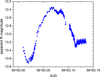 |
Fig. 1 Light curve of WO107 with the apparent magnitudes observed at Simeiz Observatory on November 29/30, 2020. |
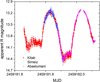 |
Fig. 2 Light curves obtained from observational data on November 28/29 during the passage of the asteroid at a minimum distance from the Earth. |
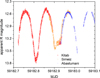 |
Fig. 3 Light curves of WO107 obtained on November 29/30, 2020. |
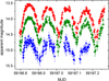 |
Fig. 4 BVR light curves of WO107 observed with the BART (FRAMORM) telescope at the Roque de los Muchachos on December 3/4, 2020. From bottom to top, the light curves show B in blue, V in green, and R in red. |
3 Shape modeling
Our photometric observations and the Goldstone radar data (Benner 2020) were used to derive the shape model of the asteroid. As the quantity of the data is limited, no fine resolution of the shape model can be obtained, and we constrained ourselves to a simple bilobal ellipsoidal shape model.
3.1 Modeling the photometric data
To model the rotation curve of the asteroid, we created a program that computes the brightness of an asteroid of a given shape and orientation. The details of this program are described in Appendix A.
The asteroid is assumed to be composed of two ellipsoidal lobes with the semi-axes a1 > b1 > c1 and a2 > b2 > c2, whose longest semi-axes a1 and a2 are aligned with each other, while c1 and c2 are parallel to the rotation axis of the asteroid (Figure 7). The asteroid rotates with the period P around the rotation axis that points at the ecliptic coordinates (λ, β). The rotation phase at the initial epoch is ϕ0.
Our program computed the brightness of the asteroid for each point of each light curve. Then, we computed the residual between the theoretical and the observed light curves,
 (1)
(1)
Here,  is the observed apparent magnitude of the asteroid, Δmij is the observational error, and
  is the theoretical apparent magnitude, determined from the light flux using Pogson’s formula. The index i lists all the Nlc observed light curves, and the index j lists all the Np points in each light curve. All the observations were treated as relative photometry, and each light curve was shifted vertically by a value si, determined in such a way as to minimize χ2, that is, from the condition ∂χ2/∂si=0. The null-point of Pogson’s formula during the computation of mth was taken arbitrarily, as its influence is canceled by the shifts si.
The free parameters of the model a1, b1, c1, a2, b2, c2, λ, β, and ϕ0 were updated by employing a Markov chain Monte Carlo (MCMC) algorithm to minimize  . For this purpose, we used the emcee package (Foreman-Mackey et al. 2013), which implements the ensemble sampler. In our case, the ensemble sampler consisted of three movers: StretchMove, DEMove, and DESnookerMove, which generate proposals for updating the coordinates of the walkers in the ensemble. The mover was chosen randomly for each step, with probabilities of 0.4, 0.3, and 0.3, respectively. The mixture of moves was chosen for an efficient sampler suited for a high-dimensional model. The sampler used 120 walkers with 50 000 steps to explore the parameter space, the first 2000 steps of which were discarded as a burn-in.
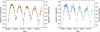 |
Fig. 5 Light curves of WO107 for the B and V filters (left) and V and R filters (right), obtained with the BART (FRAM-ORM) telescope at the Roque de los Muchachos on December 3/4, 2020. The light curves were shifted along the magnitude axis by the values of the obtained color indices. |
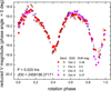 |
Fig. 6 Composite light curve of WO107 for V magnitudes reduced to zero phase angle with parameter G = 0.13 for observations at the Skalnaté Pleso on December 2 and 8. The light curves for the R band are shifted to the V light curves. |
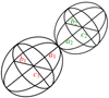 |
Fig. 7 Sketch for the shape model of WO107 we used in our simulations. It is composed of two ellipsoidal lobes. |
3.2 Modeling radar data
Delay-Doppler imaging of WO107 was conducted from Goldstone on November 28, 29, and 30, 2020 (Benner 2020). The images published on the website represent in arbitrary units the distribution of the reflected power received by the radar as a function of time delay Δ t and frequency shift Δ v.
To derive the parameters of the asteroid from its radar images, we created a program to numerically model the delayDoppler data for a given asteroid shape. The asteroid was again represented by two connected triaxial ellipsoids (see Figure 7), and a number of rays were cast on the asteroid and traced back. The numeric routine is similar to the one described in Appendix A. One of the differences is that the direction of the incoming and outgoing rays were now both aligned with the asteroid-Earth direction. Another difference is that prior to the summation of the energies of all the rays, we binned them by Δt and Δv. The third difference was another scattering law, which for radar was chosen to be proportional to cosn θ, with θ being the incidence angle, and n being a free parameter (Virkki 2024; Magri et al. 2007). Based on the results of preliminary optimization runs, the best results in terms of fitting the data were achieved for 1.75 ≤ n ≤ 2.25, which is close to the Lambert law. Thus, the value for n was set to 2. Then, the program determined the best values of the free parameters of the asteroid model, and as a result, we obtained theoretical delay-Doppler images.
This simulated radar image was then compared to the observed image. For this comparison, the two images were shifted to align their centers of mass (the median energyweighted Δ t and Δ v). The corresponding vertical and horizontal shifts were made by a rounded integer number of pixels, but this cannot cause a substantial error because the pixel size is much smaller than the size of the asteroid. As we only had access to the published radar images, we tried to transform the modeled data correspondingly to facilitate their comparison. As the published images had saturated pixels, we achieved the same effect by setting a maximum pixel brightness, adjusted to reach the best visual similarity between the modeled and observed data. Then, we compared the shifted and saturated theoretical image to the observed image pixel by pixel, and we computed the  as the sum of squared differences between the brightnesses over all the pixels of all the images.
The resulting inconsistency of the radar images  was used in an MCMC routine alongside the previously defined inconsistency of the photometric light curves
  . The ultimate MCMC fit to the data was performed via minimizing the sum
  , where the coefficient k was introduced to equalize the contribution from the photometric and radar data. It was empirically chosen in such a way that the residual values of
  and
and  for the best-fit models were nearly the same.
3.3 Resulting shape
As a result of the MCMC simulation, we obtained the distribution of the best-fit asteroid parameters. From all the values tried by the MCMC algorithm, we determined the value with the lowest χ2, and then took it for the starting value to further improve χ2 using the optimization method called differential evolution, based on Storn & Price (1997) from the package scipy.optimize10.
A sample comparison between the theoretical model and one of the observed radar images is shown in Figure 8, and a comparison with the remaining images is shown in Figure B.1 in Appendix B. The theoretical image was computed for the asteroid model with the lowest found χ2.
The comparison between the observed and simulated light curves of the asteroid is illustrated in Figure B.3 in Appendix B. Once again, the simulations were conducted for the asteroid model with the lowest χ2. The H magnitude shown in the light curve is the relative magnitude.
The best-fit model describes the photometric and radar observational data well. The photometric light curves are well fit in terms of their phase, amplitude, and overall shape. The minima of the light curves produced by self-shadowing and self-occultations of the asteroid are the most sensitive to the shape and orientation of the asteroid, and thus, they are the most crucial indicator of the fit accuracy. In most of the cases, the minima of the light curves are satisfactorily reproduced by the best-fit theoretical model. The comparison of the observed and modeled radar images demonstrates a general agreement in shape, size, and orientation, although each picture in the figures has disagreeing parts as an unavoidable result of the limitations of our theoretical model and imperfections of the observational data.
The corner plot in Figure 9 demonstrates the correlations between the results of the MCMC sampling of the six parameters that characterize the asteroid shape and the two angles that determine the orientation of its rotation axis. The diagonal subplots show the histograms of the distribution of walkers over each parameter, whereas the nondiagonal elements show the correlation in each pair of parameters.
The distribution of walkers in the MCMC simulation (Figure 9) is sensitive to the fine details of the MCMC algorithm and in general does not sample the error distribution of the parameters well. To obtain proper error estimates, we harnessed the bootstrapping method. For this sake, we rejected a randomly selected half of the light curves and a randomly selected half of the radar images and repeated the MCMC procedure to determine the least-squares model of this bootstrapped subsample. We repeated this bootstrapping procedure 300 times with statistically independent subsamples. The distribution of the best-fit parameters for the bootstrapped subsamples is shown in Figure 9.
Figure 10 shows the corresponding pole solution in the vicinity of the south pole of the ecliptic coordinates. It is a polar representation of the λ–β plot, whose Cartesian representation is shown as the seventh panel in the last row in Figure 9. Figure 10 shows that the distribution of the MCMC walkers (color coded) and the best solution for each bootstrap (red points) both cluster around two separate pole solutions, one solution centered around λ = 96°, β = −78°, and the other solution centered around λ = 286°, β = −76°. Nonunique pole solutions like this occur often in the shape modeling of asteroids (Kaasalainen & Lamberg 2006). We split the solutions into two groups, 0° < λ < 180° and 180° < λ < 360°, which visually approximately correspond to the two clusters of the bootstrapped points. Then, assuming a 2D normal distribution of errors, we computed the 1σ contour in each of the two groups of points and marked the contours with red ellipses. The solution at λ = 96°, β = −78° (reached in 65% out of 300 bootstrapped subsamples) is more plausible than the solution at λ = 286°, β = −76° (35% of subsamples), but neither of the solutions can be ruled out.
Table 3 shows the best-fit parameters of the MCMC simulation and their errors. The errors were computed as the mean-squared deviation of the best-fit parameters for the bootstrapped subsamples with respect to the full data sample.
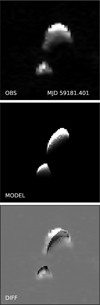 |
Fig. 8 Sample radar image. The first image represents the observed data, the second image shows the modeled data, and the third image illustrates the difference between them. For a perfect agreement between the images, the pixels of the third image would be gray, but for the worse agreement, they are split into separate shapes. |
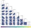 |
Fig. 9 Corner plot showing the correlation between the most important parameters of the MCMC asteroid model. The red ellipses show the 1σ contour, assuming a 2D normal distribution of errors. The moments of this distribution were estimated from the bootstrapped points. In the two bottom rows, the two red ellipses correspond to two different pole solutions. |
4 Density determination
The consideration of the gravitational equilibrium of two triaxial ellipsoids in contact allowed us to determine the density of the asteroid.
The density estimate was obtained from the condition that the gravitational attraction between the two lobes of the asteroid is equal to their centrifugal repulsion. The gravitational attraction between the two lobes of equal densities is
 (2)
(2)
We treated the gravitational field of the two ellipsoidal lobes as the gravitational field of a point mass. The accuracy of this approach is sufficient for our purposes, as we show below that the resulting density error is much greater than the error that is expected to stem from this assumption.
The distance from the second lobe to the center of mass of the binary system is
 (3)
(3)
The centrifugal force acting on this lobe is
 (4)
(4)
where ω is the angular velocity of the asteroid, and m2 is the mass of the second lobe.
We assumed force balance, Fcentr = Fgr. In reality, this condition can break in both directions. First, the centrifugal force can slightly exceed the gravitational force, Fcentr > Fgr, due to the tensile strength of the asteroid material in the contact region of the two lobes. Second, the gravity can exceed the centrifugal force, Fcentr < Fgr, due to the contact pressure between the two lobes. Still, the clear contact binary shape seen in the radar images implies a small area of contact between the two lobes, and thus, a small difference at most between the gravity and the centrifugal force. Equating the two, we obtained the density of the asteroid,
 (5)
(5)
When all the dimensions of the asteroid are multiplied by the same factor k, the numerator and denominator in Eq. (5) are both multiplied by k3, and thus, ρ remains unchanged. In this sense, the resulting asteroid density does not depend on the absolute values of the ellipsoid axes, just on their ratios.
We applied this equation to the asteroid shapes and rotation periods obtained for each of 300 bootstrapped solutions. We show the results in Figure 11. The estimates for the 1σ density error are shown with vertical green lines, while the density for the lowest χ2 value for the full sample is shown with the thick vertical line, and we assumed it for the nominal value. The plot indicates a bimodal distribution, but we cannot suggest any simple cause for this apparent bimodality. The resulting density estimated from the shape is  .
.
Asteroid parameters.
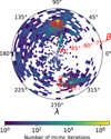 |
Fig. 10 Solutions for the pole orientation of the asteroid. The color map shows the distribution of the MCMC samples, and the red dots show the bootstrap solutions. |
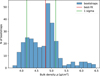 |
Fig. 11 Density estimates for WO107. The blue histogram shows the distribution of densities calculated from bootstraps. The red line shows the density estimate from the best-fit asteroid model for the full data, and the green lines show the 1σ uncertainty range estimated from the bootstrapped data. |
5 Origin and orbital evolution
To obtain information about the possible origin of the asteroid, we used the NEOPOP11 software, which is based on the debiased distribution model of near-Earth asteroids (Granvik & Brown 2018). The model suggests v6 secular resonance with Saturn to be the only possible source of the asteroid. In fact, v6 is one of the main contributors to the near-Earth asteroid population and is responsible for nearly 25% of the bodies on highly eccentric orbits similar to WO107 in magnitude (Nesvorný et al. 2023).
To obtain information about the orbital evolution of WO107, we performed numerical simulations. As the base for computation, we used GENGA, which is a hybrid symplectic N-body integrator that uses graphical processing units to integrate planet and small body dynamics (Grimm & Stadel 2014; Grimm et al. 2022).
The base of the model consisted of all the planets of the Solar System and the most massive bodies of the main asteroid belt: Ceres, Vesta, and Pallas. The asteroid was represented by 5000 and 200 000 clones, which were integrated 106 years to the past and 104 years to the near future, respectively. The Yarkovsky effect was included in the simulation.
The results of the modeling show that WO107 experiences numerous close encounters with the terrestrial planets throughout its orbital history as a consequence of its highly eccentric orbit. For the nearest 200 years into the future, integrations indicate minor interactions with Venus and Earth, which slightly raise the orbit, followed by close encounters with Venus at the 500 — year mark, Mercury at 1200, Venus at 2700, Earth at 5600–6000, and Mars at 7000–10 000 years (Figure 12). In terms of a risk assessment of WO107 as a potentially hazardous asteroid, only 250 out of 200 000 clones (0.1%) have close-encounter distances of ≤ 5 REarth, and 14 clones (0.007%) collide with the Earth (distances of ≤ REarth).
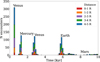 |
Fig. 12 Encounters of WO107 with terrestrial planets in the simulation to 10 kyr into the future. |
6 Discussion and conclusions
We carried out observations of WO107 from November 28 to December 6, 2020, which showed light curves typical for contact binary asteroids. The precise rotation period and maximum amplitudes of the brightness variations at a wide range of phase angles from 5 up to 68 degrees were determined.
The asteroid light curves and its radar data strongly suggested a contact binary shape. Therefore, we assumed that the asteroid is composed of two ellipsoidal lobes, fit their parameters to the observational data, and obtained a satisfactory agreement. This served as a justification of the chosen shape model, although more complicated asymmetric shape models cannot be discredited. The best-fit shape model consists of the ellipsoidal lobes with the sizes 0.68 × 0.38 × 0.36 km and 0.44 × 0.42 × 0.16 km. The asteroid rotates around its shortest axis with a rotation period of 5.017 ± 0.002 h. The most probable solution for the angular velocity vector of the asteroid points at the ecliptic coordinates λ = 96° ± 8° and β = −78° ± 1°, but another less probable solution around λ = 286° ± 11°, β = −76° ± 2° cannot be disregarded. This uncertainty in λ is largely explained by the value of β that is close to −90°, so that the ratio of the dimensions of the uncertainty area on the celestial sphere is much less extreme, as shown in Fig. 10, which gives the pole-on view of the possible positions of the asteroid pole on the celestial sphere.
From the consideration of the gravitational equilibrium of two triaxial ellipsoids in contact, we estimated the density for the asteroid,  . Interestingly, the flattening of the asteroid lobes strongly affects this high density. The result would have been about three times lower for two spheres. The resulting mass of the asteroid can be estimated as
  . The obtained high density of the asteroid can imply a substantial metal content. This agrees with the possible M taxonomic type of the asteroid.
The orbital simulation of a large number of clones of WO107 showed that it is a potentially hazardous asteroid. Numerical simulations for the next 10 000 years give an integral probability of colliding with the Earth of 7 · 10−5, with the maximum around 5900 years into the future.
Acknowledgements
This work was partially funded by the National Research Foundation of Ukraine, grant No. 2020.02/0371 “Metallic asteroids: search for parent bodies of iron meteorites, sources of extraterrestrial resources”. YK and OG thank for supporting the European Federation of Academies of Sciences and Humanities (grants ALLEA EFDS-FL1-18 and ALLEA EFDS-FL1-16, respectively) and Astronomical Observatory Institute of Faculty of Physics of Adam Mickiewicz University, where a part of the work was done. OI, MH were supported by the Slovak Grant Agency APVV no. APVV-19-0072, the Slovak Grant Agency VEGA 2/0059/22. VL acknowledges financial support from the German Excellence Strategy via the Heidelberg Cluster of Excellence (EXC 2181 – 390900948) “STRUCTURES”. The authors are grateful to A. Zhornichenko, V. Agletdinov, A. Novichonok for the help with observations and S. Mykhailova for assistance with the data reduction. The operation of FRAM-ORM telescope is supported by grants of the Ministry of Education of the Czech Republic LM2023032 and LM2023047, as well as EU/MEYS grants CZ.02.1.01/0.0/0.0/16_013/0001403, CZ.02.1.01/0.0/0.0/18_046/0016007, CZ.02.1.01/0.0/0.0/ 16_019/0000754, and CZ.02.01.01/00/22_008/0004632. Based on data from CMC15 Data Access Service at CAB (INTA-CSIC). Survey (APASS), funded by the Robert Martin Ayers Sciences Fund. This work has made use of data from the Asteroid Terrestrial-impact Last Alert System (ATLAS) project. ATLAS is primarily funded to search for near-Earth asteroids through NASA grants NN12AR55G, 80NSSC18K0284, and 80NSSC18K1575; byproducts of the NEO search include images and catalogs from the survey area. The ATLAS science products have been made possible through the contributions of the University of Hawaii Institute for Astronomy, the Queen’s University Belfast, the Space Telescope Science Institute, and the South African Astronomical Observatory. YK thanks the French PAUSE program, which provides support to scientists at risk. We are very grateful to the anonymous Referee, whose insightful critical remarks helped very much to improve the contents and the style of the article. The authors express their gratitude to all those people who defend Ukraine and thus made it possible to prepare this article.
Appendix A Computation of the asteroid brightness
We created a program that separates the binary asteroid into multiple small facets, checks which facets are illuminated by the Sun and are seen from the Earth, and adds up the scattered intensity of all the facets to calculate the total brightness of the asteroid.
For each point on the light curve, we use the JPL Horizons database to obtain the vectors connecting the asteroid with the Sun and the Earth. These vectors are then transformed from the ecliptic coordinate frame to the body-fixed coordinate frame with the equations inverse to Eq. (1) in Ďurech et al. (2010).
In the body-fixed frame, the asteroid shape model is composed of two ellipsoids, aligned with the coordinate axes and shifted along the x axis, so that the radius vector of a point on one of the ellipsoids is given in parametric form by
 (A.1)
(A.1)
Here, a, b, and c are the semimajor axes of the ellipsoid, d is the shift of the ellipsoid from the center of mass of the asteroid, α \in [0; 2 π) and β \in[−π / 2; π / 2] are two variables that parametrize the ellipsoid surface. To cover the entire surface, we sample α and β with small steps  , where N is the number of points per π / 2 radians, which in our simulations was set N = 30−50. We compute the linear parts of the changes of the radius vector between the points adjacent in longitudinal and latitudinal directions,
 (A.2)
(A.2)
 (A.3)
(A.3)
The surface element δS = δ rα × δ rβ based on vectors δ rα and δ rβ is given by
 (A.4)
(A.4)
From δS we determine the surface area δ S = |δS| and the normal vector n=δ S / δ S of each surface element.
Then the brightness created by the surface element is computed as a combination of the Lommel–Seeliger and Lambert laws in accordance with the first equation in Section 2.3 of Ďurech et al. (2010). The Lambertian part in this equation is assumed equal to 0.1, as it is done for most of the asteroids in the DAMIT database12. As we only use relative photometry, we ignore the phase function, which gives just a vertical shift to a light curve but no noticeable change in its shape. The angles in the scattering laws are computed based on the normal vector n of the surface element and the previously computed asteroid–Earth and asteroid-Sun vectors in the body-fixed frame.
The brightness created by each surface element is added to the total brightness of the asteroid only if the element is simultaneously illuminated by the Sun and seen from the Earth. It means that both the incoming and the outgoing ray lie above the local horizon and do not intersect the other lobe of the asteroid. The requirement that they lie above the local horizon is taken care of by the scattering law, whereas the condition of not intersecting the other lobe must be checked separately. To check whether a ray intersects an ellipsoid, we perform an affine transformation that turns the ellipsoid into a sphere, and then check the condition of whether the transformed ray intersects the sphere.
Thus, our program accounts for shadowing but not self-illumination of the asteroid. Still, the latter is not expected to be too important, as the albedo of the asteroid is low.
The program was subject to multiple unit tests to check if it works correctly. For one big spherical lobe and the second lobe of negligibly small size the brightness remained constant. The same was true if one spherical lobe was situated fully inside the other spherical lobe (a nonphysical case used purely as a mathematical test). For two equal spherical lobes at very large separation (wide binary asteroid), the brightness was twice as big as for one lobe. At zero phase angle the computed brightness for a Lambertian sphere agreed with the analytic result. For an arbitrary contact binary asteroid at 0 phase angle the brightness was 0. For a contact binary with the lobes 2:1:1 and 1:1:1 in equatorial aspect the light curve agreed with our physical expectations. In the polar aspect at 0 phase angle the light curve was constant, the same as the maximum in the equatorial aspect at 0 phase angle. It was also checked that the simultaneous revolution of the asteroid axis and the vectors asteroid-Sun and asteroidEarth do not change the light curve. These unit tests made us sufficiently confident that the program works correctly.
Appendix B MCMC results
In this Appendix, we present the extended plots from the optimization simulations of the asteroid parameters, samples of which were demonstrated in the main text of the article.
In Figure B.1, we show the observed images in which the observation time is indicated as modified Julian date (MJD), simulated radar images from our numeric model, and the difference between observed and modeled images. They are visualized in the same manner as in Figure 8 (see explanations of it in the main text). The total number of radar images used in our analysis was 71: 1 in Figure 8 and 70 in Figure B.1.
Figure B.3 shows all the observed light curves for the asteroid overlaid with modeled ones.
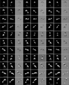 |
Fig. B.1 Observed and simulated radar images and their difference. Observed images are taken from Benner (2020). |
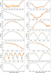 |
Fig. B.3 Comparison of observed (orange) and simulated (blue) photometric data. Zero date is JD 2459182.3299. |
References
- Belskaya, I. N., & Lagerkvist, C. I., 1996, Planet. Space Sci., 44, 78 [Google Scholar]
- Benner, L. A. M., 2020, Goldstone Radar Observations Planning: (7753) 1988 XB, 2017 WJ16, and 2000 WO107, NASA JPL database “Asteroid Radar Research”, https://echo.jpl.nasa.gov/asteroids/1988XB/1988xb.2020.goldstone.planning.html [Google Scholar]
- Binzel, R. P., Rivkin, A. S., Stuart,, et al. 2004, Icarus, 170, 259 [NASA ADS] [CrossRef] [Google Scholar]
- Binzel, R. P., DeMeo, F. E., Turtelboom, E. V., et al. 2019, Icarus, 324, 41 [Google Scholar]
- Bowell, E., Chapman, C. R., Gradie, J. C., Morrison, D., & Zellner, B., 1978, Icarus, 35, 313 [NASA ADS] [CrossRef] [Google Scholar]
- Ďurech, J., Sidorin, V., & Kaasalainen, M., 2010, A&A, 513, A46 [Google Scholar]
- Foreman-Mackey, D., Hogg, D. W., Lang, D., & Goodman, J., 2013, PASP, 125, 306 [Google Scholar]
- Franco, L., De Pieri, A., Brosio, A., et al. 2021, MPB, 48, 120 [Google Scholar]
- Granvik, M., & Brown, P., 2018, Icarus, 311, 271 [Google Scholar]
- Grimm, S. L., & Stadel, J. G., 2014, ApJ, 796, 23 [NASA ADS] [CrossRef] [Google Scholar]
- Grimm, S. L., Stadel, J. G., Brasser, R., Meier, M. M. M., & Mordasini, C., 2022, ApJ, 932, 124 [NASA ADS] [CrossRef] [Google Scholar]
- Kaasalainen, M., & Lamberg, L., 2006, InvPr, 22, 749 [Google Scholar]
- Krugly, Y. N., 2004, Sol. Syst. Res., 38, 241 [Google Scholar]
- Krugly, Y. N., Belskaya, I. N., Shevchenko, V. G., et al. 2002, Icarus, 158, 294 [NASA ADS] [CrossRef] [Google Scholar]
- Lacerda, P. 2007, ApJ, 672, L57 [Google Scholar]
- Mainzer, A., Bauer, J., Cutri, R., et al. 2019, NASA Planetary Data System, NEOWISE Diameters and Albedos V2.0, doi:10.26033/18S3-2Z54 [Google Scholar]
- Magri, C., Ostro, S. J., Scheeres, D. J., Nolan, M. C., et al. 2007, Icarus, 186, 152 [NASA ADS] [CrossRef] [Google Scholar]
- Mottola, S., De Angelis, G., Di Martino, M., et al. 1995, Icarus, 117, 62 [NASA ADS] [CrossRef] [Google Scholar]
- Nesvorný, D., Deienno, R., Bottke, W. F., et al. 2023, AJ, 166, 55 [CrossRef] [Google Scholar]
- Storn, R., & Price, K., 1997, J. Glob. Optim., 11, 341 [Google Scholar]
- Virkki, A., 2024, Remote Sensing, 16, 890 [Google Scholar]
- Warner, B. D., & Stephens, R. D., 2021, MPB, 48, 170 [Google Scholar]
- Warner, B. D., 2022, MPO Software, MPO Canopus v. 10.8, Bdw Publishing,https://minplanobs.org/BdwPub/php/mpocanopus.php [Google Scholar]
- Zappala, V., Cellino, A., Barucci, A. M., Fulchignoni, M., & Lupishko, D. F., 1990, A&A, 231, 548 [NASA ADS] [Google Scholar]
Lincoln Near-Earth Asteroid Research.
Minor Planet Center, List Of Potentially Hazardous Minor Planets, https://minorplanetcenter.net/iau/mpc.html
Near-Earth Object Wide-field Infrared Survey Explorer.
Minor Planet Center.
Burst Alert Robotic Telescope.
Minor Planet Observer.
American Association of Variable Star Observers Photometric All-Sky Survey, https://www.aavso.org/apass
Carlsberg Meridian Catalogue, http://svocats.cab.inta-csic.es/cmc15/
Asteroid Terrestrial-impact Last Alert System, https://atlas.fallingstar.com/
SciPy package: https://docs.scipy.org/
Near-Earth Object Population Observation Program.
Astronomical Institute of the Charles University, Josef Ďurech, Vojtěch Sidorin, DAMIT, https://astro.troja.mff.cuni.cz/ projects/damit
All Tables
All Figures
|
Fig. 1 Light curve of WO107 with the apparent magnitudes observed at Simeiz Observatory on November 29/30, 2020. |
| In the text | |
|
Fig. 2 Light curves obtained from observational data on November 28/29 during the passage of the asteroid at a minimum distance from the Earth. |
| In the text | |
|
Fig. 3 Light curves of WO107 obtained on November 29/30, 2020. |
| In the text | |
|
Fig. 4 BVR light curves of WO107 observed with the BART (FRAMORM) telescope at the Roque de los Muchachos on December 3/4, 2020. From bottom to top, the light curves show B in blue, V in green, and R in red. |
| In the text | |
|
Fig. 5 Light curves of WO107 for the B and V filters (left) and V and R filters (right), obtained with the BART (FRAM-ORM) telescope at the Roque de los Muchachos on December 3/4, 2020. The light curves were shifted along the magnitude axis by the values of the obtained color indices. |
| In the text | |
|
Fig. 6 Composite light curve of WO107 for V magnitudes reduced to zero phase angle with parameter G = 0.13 for observations at the Skalnaté Pleso on December 2 and 8. The light curves for the R band are shifted to the V light curves. |
| In the text | |
|
Fig. 7 Sketch for the shape model of WO107 we used in our simulations. It is composed of two ellipsoidal lobes. |
| In the text | |
|
Fig. 8 Sample radar image. The first image represents the observed data, the second image shows the modeled data, and the third image illustrates the difference between them. For a perfect agreement between the images, the pixels of the third image would be gray, but for the worse agreement, they are split into separate shapes. |
| In the text | |
|
Fig. 9 Corner plot showing the correlation between the most important parameters of the MCMC asteroid model. The red ellipses show the 1σ contour, assuming a 2D normal distribution of errors. The moments of this distribution were estimated from the bootstrapped points. In the two bottom rows, the two red ellipses correspond to two different pole solutions. |
| In the text | |
|
Fig. 10 Solutions for the pole orientation of the asteroid. The color map shows the distribution of the MCMC samples, and the red dots show the bootstrap solutions. |
| In the text | |
|
Fig. 11 Density estimates for WO107. The blue histogram shows the distribution of densities calculated from bootstraps. The red line shows the density estimate from the best-fit asteroid model for the full data, and the green lines show the 1σ uncertainty range estimated from the bootstrapped data. |
| In the text | |
|
Fig. 12 Encounters of WO107 with terrestrial planets in the simulation to 10 kyr into the future. |
| In the text | |
|
Fig. B.1 Observed and simulated radar images and their difference. Observed images are taken from Benner (2020). |
| In the text | |
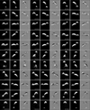 |
Fig. B.2 Observed and simulated radar images and their difference. Continuation of Fig. B.1 |
| In the text | |
|
Fig. B.3 Comparison of observed (orange) and simulated (blue) photometric data. Zero date is JD 2459182.3299. |
| In the text | |
Current usage metrics show cumulative count of Article Views (full-text article views including HTML views, PDF and ePub downloads, according to the available data) and Abstracts Views on Vision4Press platform.
Data correspond to usage on the plateform after 2015. The current usage metrics is available 48-96 hours after online publication and is updated daily on week days.
Initial download of the metrics may take a while.