| Issue |
A&A
Volume 702, October 2025
|
|
|---|---|---|
| Article Number | A153 | |
| Number of page(s) | 14 | |
| Section | Interstellar and circumstellar matter | |
| DOI | https://doi.org/10.1051/0004-6361/202452590 | |
| Published online | 16 October 2025 | |
The role of polycyclic aromatic hydrocarbons in astrochemical modeling at different evolutionary stages of cold dense cloud cores
1
Xinjiang Astronomical Observatory, Chinese Academy of Sciences,
Urumqi
830011,
China
2
Key Laboratory of Radio Astronomy, Chinese Academy of Sciences,
Urumqi
830011,
China
3
Departamento de Astronomía, Universidad de Chile,
Camino el Observatorio 1515, Las Condes,
Santiago,
Chile
4
Shanghai Astronomical Observatory, Chinese Academy of Sciences,
80 Nandan Road,
Shanghai
200030,
PR
China
5
Universidad Autónoma de Chile, Facultad de Ingeniería, Núcleo de Astroquímica & Astrofísica,
Av. Pedro de Valdivia 425,
Providencia,
Chile
6
Department of Physics, Faculty of Science, Kunming University of Science and Technology,
Kunming
650500,
PR
China
7
Yunnan Observatories, Chinese Academy of Sciences,
396 Yangfangwang, Guandu District, Kunming
650216,
Yunnan,
PR
China
8
Chinese Academy of Sciences South America Center for Astronomy, National Astronomical Observatories, CAS,
Beijing
100101,
PR
China
★ Corresponding author: This email address is being protected from spambots. You need JavaScript enabled to view it.
Received:
12
October
2024
Accepted:
6
August
2025
Abstract
Context. Although the role of PAHs have been highlighted in recent years, it is crucial to verify their functions at different evolutionary stages of dark cloud cores.
Aims. Fitting molecular abundances with gas-grain chemical models has revealed shorter chemical ages for denser cold dark cloud cores. To deepen the understanding of chemical ages and the functions of PAHs, we investigated the influence of PAHs in our chemical models by fitting observational data.
Methods. We collected observed molecular abundances (at least five species per core) from the literature for 39 cold dense cloud cores (T < 25 K and 104 ≤ nH ≤ 107 cm−3). Using a gas-grain chemical model, we fit the molecular abundances of the 39 samples to determine the best-fit chemical ages and discuss the role of PAHs in an evolutionary view.
Results. We find an anticorrelation between the gas density and the fit chemical age through molecular abundance fitting. The best-fit chemical ages of the low-density cores (<7 × 104 cm−3) are comparable to the dynamical ages, which can be a good alternative indicator of physical age. However, for high-density cores (>7 × 104 cm−3), the chemical age is far from the physical age and therefore useless. The inclusion of PAHs do not change the estimation of the chemical ages much, which indicates the small effect of PAHs on average. However, we identified molecular tracers that are sensitive to PAHs at different evolutionary stages, thus revealing their diagnostic potential for chemical evolution.
Key words: ISM: abundances / ISM: clouds / evolution / ISM: molecules
© The Authors 2025
 Open Access article, published by EDP Sciences, under the terms of the Creative Commons Attribution License (https://creativecommons.org/licenses/by/4.0), which permits unrestricted use, distribution, and reproduction in any medium, provided the original work is properly cited.
This article is published in open access under the Subscribe to Open model. This email address is being protected from spambots. You need JavaScript enabled to view it. to support open access publication.
1 Introduction
Interstellar molecular lines provide critical constraints on the evolutionary stage of star formation processes by activating different observational properties (e.g., Rawlings & Yates 2001; Herbst & van Dishoeck 2009; Agúndez & Wakelam 2013; Jørgensen et al. 2020). To interpret physical and chemical processes through molecular tracers, static gas-grain chemical models with fixed physical parameters (e.g., gas density, visual extinction, radiation field, cosmic-ray ionization rate) are widely used by incorporating comprehensive reaction networks (e.g., Hasegawa et al. 1992; Hasegawa & Herbst 1993a,b; Garrod et al. 2007; Semenov et al. 2010; Ruaud et al. 2016; Ge 2022). These models systematically yield younger chemical ages for denser cores when comparing objects (e.g., Maret et al. 2013; Tang et al. 2019), therefore contradicting physical expectations that an increased density corresponds to greater evolutionary maturity. This discrepancy obscures evolutionary sequencing across diverse objects. A clearer understanding of the chemical age of the chemical model remains necessary, even though some literature has explained this as being a result of the fixed physical parameters that accelerate the chemical processes from simulation onset (e.g., Maret et al. 2013; Tang et al. 2019). Although chemical age represents the characteristic chemical timescale under specified physical conditions, verifying its utility for estimating physical ages remains essential. This approach becomes particularly valuable when physical age constraints are unavailable and chemical data provide the only available information.
Polycyclic aromatic hydrocarbons (PAHs) constitute important components in the dark clouds that influence chemical outcomes and consequently affect derived chemical ages. Although PAH chemistry has been shown to improve agreement between chemical models and observations in dark clouds with densities of nH ~ 104 cm−3 (e.g., Wakelam & Herbst 2008; Ge et al. 2020a; Doddipatla et al. 2021), their role across different evolutionary stages of cloud cores spanning the broad density range (~104−107 cm−3) remain unexplored. Particularly for TMC-1 CP, models incorporating PAHs yield chemical ages of ~105 yr (Wakelam & Herbst 2008), whereas other studies report ages approaching 106 yr without PAHs (e.g., Vidal et al. 2017; Laas & Caselli 2019) and with PAHs (Ge et al. 2020b). This discrepancy significantly increases the uncertainty in chemical age determination. The recent detection of PAHs in dark clouds (e.g., o-C6H4, c-C9H8 in TMC-1 Cernicharo et al. 2021b; Burkhardt et al. 2021; Cernicharo et al. 2021a) and the efficient formation of PAHs in cold dark cloud conditions (e.g., Kaiser et al. 2022) add to the evidence that PAHs exist. This has motivated us to investigate the role of PAHs in wide physical conditions and to verify its effects on the determination of chemical ages and the changing of molecular abundances.
To investigate the role of PAHs from a view of fitting observations, we collected multiple molecular abundances in a sample of 39 cold dark cloud sources and fit the samples with a gas-grain model with consideration of PAHs. This paper is organized as follows. In Section 2, the observed samples are presented. In Section 3, the physical and chemical models are described. In Section 4, the results are presented by comparing with observations. Section 5 gives our discussions. Finally, Section 6 provides a summary.
Parameters of the samples.
2 Observed samples
In order to investigate the chemical ages of low-mass dense cores via the astro-chemical models, we collected observed abundances and gas densities from literature for a sample of cold dense cores. The sources are typically cold dark cloud cores that have gas densities ranging from ~104 to 107 cm−3, temperatures lower than 20 K, and multiple observed molecular lines. The sources include TMC-1 CP and L134N (e.g., Agúndez & Wakelam 2013); L1521E (e.g., Hirota et al. 2002; Nagy et al. 2019); L1498 and L1517B (e.g., Tafalla et al. 2004, 2006); B68 (e.g., Di Francesco et al. 2002; Amin & El-Nawawy 2005); L1544 (e.g., Caselli et al. 1999; Crapsi et al. 2007; Vastel et al. 2018; Chacón-Tanarro et al. 2019; Nagy et al. 2019); and Planck Galactic Cold Clumps (PGCCs) (e.g., Tang et al. 2019; Yi et al. 2018; Liu et al. 2019; Yi et al. 2021; Wakelam et al. 2021) with T ~ 10–20 K (e.g., Planck Collaboration XXIII 2011; Planck Collaboration XXVIII 2016; Mannfors et al. 2021). The information of the collected objects is listed in Table 1. In Appendix A, a detailed description of each object can be found, with the two most important points being the following: (1) The determined chemical ages are around a few 105 yr, although younger ages (a few 104 yr) are proposed for TMC-1 CP, L1498, and L1544 using a so-called general model (Chen et al. 2022). This means that the determined chemical ages are generally subject to large uncertainties. (2) They have masses of ~1–3 M⊙, which can be classified as the same type of low-mass dense cores (M < 8 M⊙). The molecular abundances observed in all objects are listed in Tables A.1 and A.2 of Appendix A.
To summarize, our sample contains 39 objects, including seven well-known sources and 32 PGCCs. The common molecular species across the sample are N2H+, HCO+, C2H, HCN, and H2CO. Some of these seven well-known objects also show additional molecules, including CO, S-bearing species, N-bearing species, and carbon-chain molecules. We note that observational uncertainties, which are typically approximately of a factor of two, are not considered in this analysis, as these depend on the telescope beam used for observations.
Physical parameters of the chemical models.
3 Physical and chemical models
3.1 Physical parameters
The static astro-chemical model with fixed physical parameters is widely used to simulate interstellar cloud chemistry because of its minimal physical parameter requirements for cloud cores and its good agreement with observations (e.g., Hasegawa et al. 1992; Hasegawa & Herbst 1993a,b; Garrod et al. 2007; Semenov et al. 2010; Agúndez & Wakelam 2013; Ruaud et al. 2016; Ge et al. 2016b,a; Ge 2022). We adopted this approach, wherein all physical parameters remain fixed while the chemistry evolves over the cloud age. The physical parameters used (Table 2) represent typical values for cold dark cloud cores. To test gas density effects, we varied this parameter between 104 and 107 cm−3 following Section 3.4. To verify PAH effects, we performed two model types, namely, with and without PAHs.
3.2 Chemical parameters
Generally, there are two typical sets of initial abundances (relative to H2): low- (ℒ) and high-metal (ℋ) sets (e.g., Wakelam & Herbst 2008). A key distinction in the ℒ set is the depleted sulfur abundance (~8 × 10⁻⁸) compared to the cosmic value (1.5 × 10⁻⁵) adopted in ℋ sets (e.g., Lodders 2003; Asplund et al. 2009). Considering recent observational constraints proposing S-abundances of 0.4–2.2 × 10⁻⁶ in TMC-1 CP (Fuente et al. 2019) and noting that recent models using ℋ abundances achieve good agreement (e.g., Vidal et al. 2017; Laas & Caselli 2019), we employed a modified high-metal abundance set with an intermediate sulfur initialization X(S+) = 10−6. For simplicity, we indicate the set used in this work as ℳ and list the initial abundances in Table 3. The choice of the ℳ set is supported by the discussion in Section 5.1, which shows better agreements to the observed samples than the models with ℒ and ℋ sets. For all of our models, the reactive desorption proposed by Garrod et al. (2007) is used with a = ν/νs = 0.01, where ν and νs are the bond frequency of surface molecule and the frequency at which energy is transferred to the grain surface, respectively.
Initial abundances.
3.3 Code and chemical reaction network
To numerically simulate the physical and chemical processes, the GGCHEMPY1 code (Ge 2022) was modified and used. The Python package scipy.integrate.ode was used to perform the integration using the backward-differentiation formulas method.
We used the two-phase gas-grain reaction network from Semenov et al. (2010), which is available in the Kinetic database for astrochemistry (KIDA2) (Wakelam et al. 2012). With the aim of checking the effects of PAHs on chemistry, we used the PAH reaction network and the standard initial abundance (Xi(PAH) = 3.07 × 10⁻⁷) and size (rPAH = 4 Å) of PAHs from Wakelam & Herbst (2008). The gas-phase reaction network of PAH includes electron attachment (PAH + e− → PAH− + hν); recombination of PAH− with smaller positive ions (PAH− + X+ → PAH + X, in which X should be replaced by X′ + H if X+ contains hydrogen); and photodetachment of PAH− (PAH− + hν → PAH + e−) by ultraviolet, visible, and even near-infrared photons (Wakelam & Herbst 2008). Following Ge et al. (2020a), we also considered accretion (PAH → JPAH; the prefix “J” indicates a dust grain surface species) and desorption (JPAH → PAH) of PAHs with an estimated binding energy through the proposed relation by Kamp et al. (2017). In addition, for the same consideration as Ge et al. (2020a), we added 13 missed gas-phase reactions for HNCO and removed 13 unnecessary reactions as listed in their Table A1.
3.4 Model grid
To find the best fit by fitting the observations, we constructed a model grid with varied densities but a fixed extinction, AV = 10 mag; radiation field, χ = 1 χ0; and cosmic-ray ionization rate (CRIR), ζ = 1.3 × 10⁻¹⁷ s−1. The grid has ten linearly spaced densities across three density ranges of 104−105, 105−106, and 106−107 cm−3. Thus, the grid has 28 models after removing duplicates. When PAH chemistry is included, the number of models doubles.
4 Results
In this section, by fitting the observed samples with models, we present the agreements of the chemical models to observations and discuss the role of PAHs. In addition, we provide predictions of molecular tracers for observations in the future.
4.1 The agreements to observations
We used the average difference defined below to quantify the agreement between the models and observations:
![Mathematical equation: $\[\bar{D}(t)=\frac{\sum_i^N\left|\log \left(X_i^{\text {obs }}\right)-\log \left(X_i^{\bmod }(t)\right)\right|}{N}.\]$](/articles/aa/full_html/2025/10/aa52590-24/aa52590-24-eq1.png) (1)
(1)
Here, N is the number of species with the observed abundances (![Mathematical equation: $\[X_{i}^{\text {obs}}\]$](/articles/aa/full_html/2025/10/aa52590-24/aa52590-24-eq2.png) ) of species i. The
) of species i. The ![Mathematical equation: $\[X_{i}^{\text {mod}}\]$](/articles/aa/full_html/2025/10/aa52590-24/aa52590-24-eq3.png) (t) is the modeled abundance of the corresponding species at the model time, t. The smaller
(t) is the modeled abundance of the corresponding species at the model time, t. The smaller ![Mathematical equation: $\[\bar{D}\]$](/articles/aa/full_html/2025/10/aa52590-24/aa52590-24-eq4.png) (t) is, the better the overall agreement is. Thus, the best agreement is found at tbest with minimum
(t) is, the better the overall agreement is. Thus, the best agreement is found at tbest with minimum ![Mathematical equation: $\[\bar{D}_{\text {min}}\]$](/articles/aa/full_html/2025/10/aa52590-24/aa52590-24-eq5.png) . The derived Dmin value exhibits insensitivity to molecular counts in our sample, as we utilized at least five molecules (up to 54 in TMC-1 CP) to jointly constrain the models. This robustness is further confirmed by the well fit linear correlation between chemical ages and densities shown in Fig. 2. However, when fewer than five molecules are employed, Dmin becomes increasingly sensitive to the number of molecules. Consequently, reduced molecular counts progressively compromise the accuracy of the determination.
. The derived Dmin value exhibits insensitivity to molecular counts in our sample, as we utilized at least five molecules (up to 54 in TMC-1 CP) to jointly constrain the models. This robustness is further confirmed by the well fit linear correlation between chemical ages and densities shown in Fig. 2. However, when fewer than five molecules are employed, Dmin becomes increasingly sensitive to the number of molecules. Consequently, reduced molecular counts progressively compromise the accuracy of the determination.
Using Eq. (1), we fit the observed abundance with the model grid by searching for ![Mathematical equation: $\[\bar{D}_{\text {min}}\]$](/articles/aa/full_html/2025/10/aa52590-24/aa52590-24-eq6.png) in a 2D space of density and model age (see details in Appendix B). We found anticorrelations between the best-fit chemical age and gas density (see Eq. (B.1)) that can be quickly used to determine the comparable abundances to observations. This correlation is not sensitive to the PAH chemistry. From the perspective of fitting observations, the models with PAHs do not differ significantly from those without PAHs with a similar
in a 2D space of density and model age (see details in Appendix B). We found anticorrelations between the best-fit chemical age and gas density (see Eq. (B.1)) that can be quickly used to determine the comparable abundances to observations. This correlation is not sensitive to the PAH chemistry. From the perspective of fitting observations, the models with PAHs do not differ significantly from those without PAHs with a similar ![Mathematical equation: $\[\bar{D}_{\text {min}}\]$](/articles/aa/full_html/2025/10/aa52590-24/aa52590-24-eq7.png) ~ 0.5–1.0 (see Fig. 1). The objects TMC1-CP, L134N, L1521E, B68, and some PGCCs (about 69%, or 22/32) show a preference for models with PAHs, with a smaller Dmin reached. In total, ~67% (26/39) of the samples prefer the models with PAHs. We note that the modest enhancements (up to ΔDmin ~ 0.23, a factor of about 1.7) caused by PAHs are not conclusive evidence of the presence of PAHs but only highlight their positive roles in fitting the observations.
~ 0.5–1.0 (see Fig. 1). The objects TMC1-CP, L134N, L1521E, B68, and some PGCCs (about 69%, or 22/32) show a preference for models with PAHs, with a smaller Dmin reached. In total, ~67% (26/39) of the samples prefer the models with PAHs. We note that the modest enhancements (up to ΔDmin ~ 0.23, a factor of about 1.7) caused by PAHs are not conclusive evidence of the presence of PAHs but only highlight their positive roles in fitting the observations.
4.2 The chemical ages
By comparing the models with observations, we could directly constrain the chemical age that reflects the reaction timescales under a given physical condition. In this section, we investigate whether the chemical age could be an indicator of the physical age.
To do so, we used a modified free-fall collapsing models (Spitzer 1978; Nejad et al. 1990; Rawlings et al. 1992), which provides a reference true age of a collapsing dense core with 1 M⊙ and an initial density of n0 = 3000 cm−3. Fig. 2 shows the linear correlation defined in Eq. (B.1) with the solid line, which is not sensitive to the inclusion of PAHs, as seen in the last panel of Fig. B.1. This correlation predicts ages comparable to the reference physical ages of the collapsing core at densities less than ~7 × 104 cm−3 regardless of the values of B(≤ 1) – a constant that represents the braking effects of turbulence and the magnetic field – if a factor of two of the uncertainty of the fit correlation is considered to cover all the observed data points taken from the last panel of Fig. B.1. Thus, the best-fit chemical ages for low-density cores (<7 × 104 cm−3) could be a good indicator of the physical age when comparing models with observations. However, the predicted chemical ages of high-density cores (>7 × 104 cm−3) are too young to be the true ages of the cores and cannot be used to estimate the physical age.
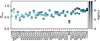 |
Fig. 1 Comparison of |
![Mathematical equation: $\[\bar{D}_{\text {min}}\]$](/articles/aa/full_html/2025/10/aa52590-24/aa52590-24-eq8.png)
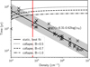 |
Fig. 2 Comparison between the best-fit chemical ages (black solid line; the formula labeled) and the ages from a modified free-fall collapse model with different B values for a 1 M⊙ cloud core (dotted, dashed, and dash-dotted lines). The gray region indicates an area twice that of the fit ages in order to cover the best-fit data points (black crosses) taken from Fig. B.1. The red vertical lines indicates a density of 7 × 104 cm−3. |
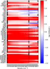 |
Fig. 3 Abundance ratios (log[X(PAH)/X]) between the models with and without PAHs as a function of density. The ratios were calculated at the best-fit ages estimated through Eq. (B.1). The filled points, empty points, and crosses indicate the species in TMC-1 CP and L1544 that prefer the model with PAHs, prefer the model without PAHs, and have a non-detection in observations, respectively. The unfilled squares mark the species that are preferred by the models with and without PAHs. All the points with symbols except those with crosses indicate that the modeled abundances are within one order of magnitude of the observed ones. |
4.3 The role of PAHs
To explore the role of PAHs in the models, we focused on the differences between the models without and with PAHs at the best-fit ages for observations. At the fit ages found through Eq. (B.1), we calculated the abundance ratios of selected species from models with and without PAHs. Fig. 3 shows the calculated logarithmic ratios (log[(X(PAH)/X]) for species that both exist in observations and in the reaction network. Comparisons between the models and two typical sources of TMC-1 CP and L1544 are shown for discussion. For TMC-1 CP, the density was determined to be about 1.5 × 104 cm−3 (Fuente et al. 2019). Thus we only compare TMC-1 CP with the models of nH = 104 cm−3. For L1544, the density was determined to be about 106−107 cm−3 (Caselli et al. 2019). Considering that our best fit for L1544 is at nH ~ 2 × 106 cm−3, we considered two models (nH = 2 × 10⁶ and 107 cm−3) to compare with the observations in order to discuss possible effects.
Figure 3 shows that the inclusion of PAHs enhances the abundances (indicated in red) of most species. For a clearer discussion, we categorized the species in Fig. 3 into three groups:
Group (1): most of the complex species with an atom number larger than four (e.g., C3O, C3H2, C5H, C6H, C8H, C5N, HNC3, H2CN, HC2NC, HC5N, HC7N, HC9N, CH3C5N, CH3C4H, CH3C6H, C2H4O, and HCNH+) have enhanced abundances across the entire density range (104−107 cm−3). This can be understood as being the result of cumulative effects since they are species with low abundances that can be enhanced by a large factor through a small change of their parent species when PAHs are considered.
Group (2): some species have enhanced abundances at low densities (nH≲105 cm−3) but reduced abundances at high densities, such as OH, C2H, C3H, C4H, CN, NO, HCN, and HNC, which are simple carbon-chain or N-bearing or O-bearing species. The reason for these behaviors are mainly due to depletion effects. At a low density of 104−105 cm−3, the depletion timescale (tdep = nH * Rd2g/Vth4 * πa2) is estimated to be about 106 yr, which is too long to take effect compared to the best-fit chemical ages of the same order as ~106 yr. However, at a high density of 106−107 cm−3, the depletion timescale is about 104 yr, which becomes comparable at >2 × 106 cm−3. Thus, depletion decreased the species abundances in the gas-phase before the best-fit chemical age. This happens to simple species rather than complex species due to the fact that the rare complex species in group (1) are more sensitive to abundance changes caused by their parent species, but not the depletion effects. We highlight here that the behaviors of these species are a result of the inclusion of PAHs but not a direct result of depletion, although the depletion timescale plays an important role in the chemical evolution.
Group (3): the species are not sensitive to PAHs. A typical case in this group is CO. This is due to the fact that its abundance (~10−4) is too high to be impacted by the chemistry of a rare species such PAHs (~10−7).
From the view in fitting observations (see symbols in Fig. 3), we see that most species (~59%, 32/54) observed in TMC-1 CP prefer the model with PAHs, especially for the species in Group (1). However, for L1544, about 27–61% (7–16/26) of the species prefer the models with PAHs, but it is difficult to discuss the role of PAHs at a high density of 106−107 cm−3. The species observed in both TMC-1 CP and L1544 that prefer the models with PAHs are NH3, HCN, HC3N, HCS+, and NS+.
The abundance enhancements due to PAHs over the entire density range of 104−107 cm−3 generally agree with previous conclusions in a model with a typical density of 104 cm−3 (Wakelam & Herbst 2008; Ge et al. 2020a). However, reduced abundances at higher densities are noted for simple species, such as CN, HCN, HNC, NH3, OH, C2H, C3H, and C4H in the models with PAHs. Among them, NH3 and HCN in the model with PAHs appear to match observations better in L1544 but at different densities. This suggests that N-bearing species (such as HCN and NH3) could be tracers of PAHs with enhanced and reduced abundances caused by PAHs at different densities.
To provide a predicted list of species abundances at typical gas densities (104, 105, 106, and 107 cm−3) with or without consideration of PAHs, we assembled Table B.2 for the static models at the corresponding fit ages via Eq. (B.1). As we have mentioned above, we compared abundances with observations in TMC-1 CP and L1544 by adopting one model with 104 cm−3 and two models with 2 × 10⁶ and 107 cm−3. By checking the reproduction fractions of the models, we observed that the static models with PAHs produce a better fit to TMC-1 CP ([23 → 36]/54) but a worse fit to L1544 ([15 → 12]/26 at nH = 106 cm−3 as seen in Table B.2) by reproducing species abundances. At a higher density of nH = 107 cm−3 for L1544, a better fit is reached by the model with PAHs [8 → 12]/26). The reproduction percentage for TMC-1 CP reaches ~70% when the best-fitting model is taken into consideration, highlighting the role of PAHs. Due to the tiny discrepancies between the models with and without PAHs and the uncertainty of density, we are unable to draw any conclusions about the role of PAHs in L1544.
Considering PAH depletion, we note that PAHs have a reduced effect in high-density cores compared to low-density cores. Fig. 4 shows that the depletion timescale of PAHs (~103 yr, red lines) in a high-density core (nH = 107 cm−3) is significantly shorter than the best-fit chemical age (~104 yr). In contrast, for a low-density core (nH = 104 cm−3, blue lines), the PAH depletion timescale (~106 yr) is comparable to the best-fit chemical age, ranging from ~7 × 10⁵ yr to 106 yr (see Fig. 2). Therefore, for high-density cores, models with and without PAHs are both possible, as discussed above for L1544.
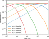 |
Fig. 4 Abundance evolutionary tracks of PAH in the gas-phase (solid) and on the dust grain surface (dashed) in the cores with selected density (see legends with different colors). |
5 Discussion
5.1 Effects of initial abundances
To examine the effects of the initial abundances of elements, we tested models with the ℒ and ℋ sets listed in Table 3 to fit the observed samples using the same method described in Section 4.1. The best-fit Dmin values are shown in Fig. 5 for models without (black) and with (cyan) PAHs. The results show that the values of Dmin are generally larger those (~0.5–0.8) from the models with the ℳ set in Fig. 1 regardless of PAH inclusion. This demonstrates that the use of the initial abundances of the ℳ set is a better choice for fitting observations.
The fit linear correlations between model ages and densities are shown in Fig. 6, which presents similar results as derived from the models with the ℳ set as in Eq. (B.1). This means that the changes of the initial abundances do not change the discussions of the role of PAHs much based on this correlation. In other words, the role of PAHs discussed in the main content of this work is the most reliable among the models with different initial abundances. We highlight that the linear correlations in models employing the ℋ parameter set (dotted lines in Fig. 6) exhibit a greater sensitivity to PAHs than those using ℳ and ℒ. Consequently, particular caution is warranted when specifying initial abundances that substantially deviate from the optimal ℳ configuration.
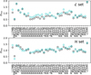 |
Fig. 5 Same as Fig. 1 but for models with the low-metal (ℒ, upper panel) and high-metal (ℋ, upper panel) sets. The black and cyan colors indicate models without and with PAHs respectively. |
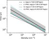 |
Fig. 6 Fit linear correlation between log(t) and log(nH) using the models with the ℒ (dashed lines) and ℋ sets (dotted lines) without (black color) and with PAHs (cyan color). The solid black line shows the fit correlation of the models with the ℳ set (see Eq. (B.1)). The gray region indicates an area twice that of the fit ages as the same as that in Fig. 2. |
5.2 Effects of reaction network
The fit results may vary based on the reaction networks developed by different researchers. Some public codes and reaction networks can be found in astrochemistry databases, such as Nahoon in KIDA and rate13 in UMIST. However, these two models feature purely gas-phase reactions, and thus they lack the dust-related processes. For a quick test, we adopted the gas-grain reaction network independently developed by Sipilä et al. (2015). The reaction network used by GGCHEMPY is based on the network of osu_03_2008 (Semenov et al. 2010), whereas the network of Sipilä et al. (2015) is based on osu_01_2009 with additional improvements in spin-chemistry for some species. We combined the network of Sipilä et al. (2015) with our code GGCHEMPY to achieve good agreement with their benchmarking models and to fit the observed samples in this work. Fig. 7 shows the fit correlation between density and time (dashed line), which compares to the fit result (solid line) shown in Eq. (B.1) within a factor of about 2.0. The values of Dmin ~ 0.4–0.8 are comparable to those in the models used in this study. These results demonstrate that the fit correlation is not sensitive to the reaction network. We note that we did not test the effects of PAHs in the reaction network of Sipilä et al. (2015) since the fit correlation shows limited sensitivity to PAHs, as can be seen in the last panel of Fig. B.1 with the black and cyan lines.
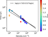 |
Fig. 7 Fit correlation between the density and time (dashed line) using the reaction network from Sipilä et al. (2015). The solid line shows the fit result in Eq. (B.1). |
5.3 The gas densities and molecular abundances
Generally, the used gas density for the chemical model is derived from the observation, which is referred to as the beam-averaged gas density (nH). Although, the model is a single-point model, the modeled abundance is suitable for the comparison because the beam effect is already taken into account through the use of the beam-averaged gas density as input. To determine the uncertainty in estimating the gas density, we made 1000 spherical cores with the Plummer-like density profile n(r) = nc/[1 + (r/a)2](p/2) (Plummer 1911), by sampling nc = 104 − 107 cm−3 (centeral density), a = 0.01–0.1 pc (inner flat region), and p = 1.5–4.5 (power-law index), and a fixed radius of R = 0.15 pc. Two beam sizes of 20 and 40 arcsec were tested to obtain beam-convolved column density profiles. Considering the strong degeneracy between a and p (e.g., Zucker et al. 2021), we adopted the analytic profile from Dapp & Basu (2009) with a fixed p = 2 to fit the column density profiles, which is a good approximation for estimating cold cloud core parameters (e.g., Tang et al. 2018). The test (see Fig. 8) showed that the determined gas density is generally (~>80%) smaller than the true one by a factor of up to approximately two for a beam of 20 arcsec and roughly four for a beam of 40 arcsec. This means that the beam effect (20–40 arcsec) results in an uncertainty of a factor of about two to four when estimating the gas density. For molecular abundances, similar behaviors are expected that could introduce such an uncertainty in the fitting process if we used true gas density as input. However, we used the beam-averaged gas density, which reduces the uncertainty to a low level. Another factor related to the gas density is the mass of the core. Considering a low-mass core with a higher mass corresponds to a higher density through accretion during the collapsing, we stress that the best chemical age could be shorter than a core with a lower density. The uncertainty caused by mass should be similar to that of the gas density.
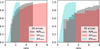 |
Fig. 8 Cumulative probability of the ratio between the true and the beam-convolved parameters (N/Nconv, n/nconv and a/aconv) for the test cores with beams of 20 (left) and 40 arcsec (right). (See details in text.). |
6 Summary
To investigate the effects of PAHs in the determination of chemical ages, the gas-grain chemical models with and without PAHs were adopted to fit molecular abundances of a large sample of 39 observed cold dense cores (T < 20 K and 104 ≤ nH ≤ 107 cm−3). The sample comprises seven well-known objects and 32 PGCCs, each with at least five detected molecular species. We summarize the key findings below.
By fitting the observed sample, we established an empirical linear correlation between the logarithmic fit gas densities (log(nH)) and chemical ages (log(t)). This correlation yields ages comparable to the physical age of a collapsing core for low-density cores (nH ≲ 7 × 104 cm−3). However, for high-density cores (nH ≳ 7 × 104 cm−3), the fit ages are too young to be the true age of a collapsing core. This correlation exhibits no sensitivity to PAH inclusion when the optimized initial abundances (ℳ set used in this work) for dark clouds are used. It also remains insensitive to the reaction networks. The correlation thus provides a basic understanding of the estimated chemical ages from a modeling perspective.
Based on the fit correlation, the role of PAHs was investigated from an evolutionary perspective by fitting multiple observed samples. About 67% of the samples prefer the models with PAHs, highlighting PAH significance. We find that PAHs introduce different abundance effects at different gas densities, extending previous conclusions for low-density cores (nH ~ 104 cm−3). Our results show similar enhanced abundances in low-density cores (~104 to a few 105 cm−3) due to PAH inclusion. However, we noted reduced abundances for some species in high-density cores (> a few 105 cm−3) due to the balance between the depletion effects and the enhancements caused by PAHs. These species, such as HCN and NH3, could be used as tracers of PAHs. We have provided a table comparing gas-phase species abundances with and without PAHs at typical gas densities.
This work provides a basic perspective on astro-chemical models through the fitting of observations. However, current gas densities and abundances derived from observations typically have large uncertainties due to large telescope beam sizes, requiring high-resolution observations (e.g., ALMA) to accurately constrain models in the future. For the chemical models, we did not consider cloud core evolutionary morphologies nor PAH sizes and structures, which could affect molecular abundances. This requires further development of a more reasonable reaction network for the chemical model.
Acknowledgements
J.X.G. thanks the Xinjiang Tianchi Talent Program (2024) and the Natural Science Foundation of Xinjiang No. 2025D01D49. NI gratefully acknowledges support from the PCI-ANID International Networks Grant REDES 190113 and FONDECYT Grant 1241193. Tie Liu acknowledges the supports by National Natural Science Foundation of China (NSFC) through grants No. 12073061 and No. 12122307, the international partnership program of Chinese Academy of Sciences through grant No.114231KYSB20200009, and Shanghai Pujiang Program 20PJ1415500. This work was partly accomplished with the support from the Chinese Academy of Sciences (CAS) through a Postdoctoral Fellowship administered by the CAS South America Center for Astronomy (CASSACA) in Santiago, Chile. This work is supported by the ChinaChile Joint Research Fund (CCJRF No. 2211) and CASSACA Key Research Project E52H540201. CCJRF is provided by Chinese Academy of Sciences South America Center for Astronomy (CASSACA) and established by National Astronomical Observatories, Chinese Academy of Sciences (NAOC) and Chilean Astronomy Society (SOCHIAS) to support China-Chile collaborations in astronomy. This study is (partly) supported by the Tianchi Talent Program of Xinjiang Uygur Autonomous Region.
References
- Agúndez, M., & Wakelam, V. 2013, Chem. Rev., 113, 8710 [Google Scholar]
- Amin, M. Y., & El-Nawawy, M. S. 2005, New A, 11, 138 [Google Scholar]
- Asplund, M., Grevesse, N., Sauval, A. J., & Scott, P. 2009, ARA&A, 47, 481 [NASA ADS] [CrossRef] [Google Scholar]
- Burkhardt, A. M., Long Kelvin Lee, K., Bryan Changala, P., et al. 2021, ApJ, 913, L18 [NASA ADS] [CrossRef] [Google Scholar]
- Caselli, P., Walmsley, C. M., Tafalla, M., Dore, L., & Myers, P. C. 1999, ApJ, 523, L165 [Google Scholar]
- Caselli, P., Pineda, J. E., Zhao, B., et al. 2019, ApJ, 874, 89 [NASA ADS] [CrossRef] [Google Scholar]
- Cernicharo, J., Agúndez, M., Cabezas, C., et al. 2021a, A&A, 649, L15 [NASA ADS] [CrossRef] [EDP Sciences] [Google Scholar]
- Cernicharo, J., Agúndez, M., Kaiser, R. I., et al. 2021b, A&A, 652, L9 [NASA ADS] [CrossRef] [EDP Sciences] [Google Scholar]
- Chacón-Tanarro, A., Pineda, J. E., Caselli, P., et al. 2019, A&A, 623, A118 [NASA ADS] [CrossRef] [EDP Sciences] [Google Scholar]
- Chen, L.-F., Chang, Q., Wang, Y., & Li, D. 2022, MNRAS, 516, 4627 [NASA ADS] [CrossRef] [Google Scholar]
- Crapsi, A., Caselli, P., Walmsley, M. C., & Tafalla, M. 2007, A&A, 470, 221 [NASA ADS] [CrossRef] [EDP Sciences] [Google Scholar]
- Dapp, W. B., & Basu, S. 2009, MNRAS, 395, 1092 [NASA ADS] [CrossRef] [Google Scholar]
- Di Francesco, J., Hogerheijde, M. R., Welch, W. J., & Bergin, E. A. 2002, AJ, 124, 2749 [NASA ADS] [CrossRef] [Google Scholar]
- Dickens, J. E., Irvine, W. M., Snell, R. L., et al. 2000, ApJ, 542, 870 [CrossRef] [Google Scholar]
- Doddipatla, S., Galimova, G. R., Wei, H., et al. 2021, Sci. Adv., 7, eabd4044 [Google Scholar]
- Draine, B. T. 1978, ApJS, 36, 595 [Google Scholar]
- Fuente, A., Navarro, D. G., Caselli, P., et al. 2019, A&A, 624, A105 [NASA ADS] [CrossRef] [EDP Sciences] [Google Scholar]
- Garrod, R. T., Wakelam, V., & Herbst, E. 2007, A&A, 467, 1103 [NASA ADS] [CrossRef] [EDP Sciences] [Google Scholar]
- Ge, J. 2022, RAA, 22, 015004 [Google Scholar]
- Ge, J. X., He, J. H., & Li, A. 2016a, MNRAS, 460, L50 [Google Scholar]
- Ge, J. X., He, J. H., & Yan, H. R. 2016b, MNRAS, 455, 3570 [Google Scholar]
- Ge, J., Mardones, D., Inostroza, N., & Peng, Y. 2020a, MNRAS, 497, 3306 [Google Scholar]
- Ge, J. X., Mardones, D., He, J. H., et al. 2020b, ApJ, 891, 36 [Google Scholar]
- Giers, K., Spezzano, S., Alves, F., et al. 2022, A&A, 664, A119 [NASA ADS] [CrossRef] [EDP Sciences] [Google Scholar]
- Hasegawa, T. I., & Herbst, E. 1993a, MNRAS, 261, 83 [Google Scholar]
- Hasegawa, T. I., & Herbst, E. 1993b, MNRAS, 263, 589 [Google Scholar]
- Hasegawa, T. I., Herbst, E., & Leung, C. M. 1992, ApJS, 82, 167 [Google Scholar]
- Herbst, E., & van Dishoeck, E. F. 2009, ARA&A, 47, 427 [NASA ADS] [CrossRef] [Google Scholar]
- Hirota, T., Ito, T., & Yamamoto, S. 2002, ApJ, 565, 359 [NASA ADS] [CrossRef] [Google Scholar]
- Ivlev, A. V., Silsbee, K., Sipilä, O., & Caselli, P. 2019, ApJ, 884, 176 [Google Scholar]
- Jiménez-Serra, I., Vasyunin, A. I., Spezzano, S., et al. 2021, ApJ, 917, 44 [CrossRef] [Google Scholar]
- Jørgensen, J. K., Belloche, A., & Garrod, R. T. 2020, Annu. Rev. Astron. Astrophys., 58, 727 [Google Scholar]
- Kaiser, R. I., Zhao, L., Lu, W., et al. 2022, Phys. Chem. Chem. Phys. (Incorp. Faraday Trans.), 24, 25077 [Google Scholar]
- Kamp, I., Thi, W.-F., Woitke, P., et al. 2017, A&A, 607, A41 [NASA ADS] [CrossRef] [EDP Sciences] [Google Scholar]
- Keto, E., & Caselli, P. 2010, MNRAS, 402, 1625 [Google Scholar]
- Keto, E., Caselli, P., & Rawlings, J. 2014, MNRAS, 446, 3731 [Google Scholar]
- Kirk, J. M., Ward-Thompson, D., & André, P. 2005, MNRAS, 360, 1506 [NASA ADS] [CrossRef] [Google Scholar]
- Laas, J. C., & Caselli, P. 2019, A&A, 624, A108 [NASA ADS] [CrossRef] [EDP Sciences] [Google Scholar]
- Lai, S.-P., Velusamy, T., Langer, W. D., & Kuiper, T. B. H. 2003, Astron. J., 126, 311 [Google Scholar]
- Lattanzi, V., Bizzocchi, L., Vasyunin, A. I., et al. 2020, A&A, 633, A118 [NASA ADS] [CrossRef] [EDP Sciences] [Google Scholar]
- Liu, X. C., Wu, Y., Zhang, C., et al. 2019, A&A, 622, A32 [EDP Sciences] [Google Scholar]
- Lodders, K. 2003, ApJ, 591, 1220 [Google Scholar]
- Makiwa, G., Naylor, D. A., van der Wiel, M. H. D., et al. 2016, MNRAS, 458, 2150 [NASA ADS] [CrossRef] [Google Scholar]
- Mannfors, E., Juvela, M., Bronfman, L., et al. 2021, A&A, 654, A123 [NASA ADS] [CrossRef] [EDP Sciences] [Google Scholar]
- Maret, S., & Bergin, E. A. 2007, ApJ, 664, 956 [Google Scholar]
- Maret, S., Bergin, E. A., & Tafalla, M. 2013, A&A, 559, A53 [NASA ADS] [CrossRef] [EDP Sciences] [Google Scholar]
- Nagy, Z., Spezzano, S., Caselli, P., et al. 2019, A&A, 630, A136 [NASA ADS] [CrossRef] [EDP Sciences] [Google Scholar]
- Navarro-Almaida, D., Fuente, A., Majumdar, L., et al. 2021, A&A, 653, A15 [NASA ADS] [CrossRef] [EDP Sciences] [Google Scholar]
- Nejad, L. A. M., Williams, D. A., & Charnley, S. B. 1990, MNRAS, 246, 183 [NASA ADS] [Google Scholar]
- Padovani, M., Walmsley, C. M., Tafalla, M., Galli, D., & Müller, H. S. 2009, A&A, 505, 1199 [NASA ADS] [CrossRef] [EDP Sciences] [Google Scholar]
- Planck Collaboration XXIII. 2011, A&A, 536, A23 [NASA ADS] [CrossRef] [EDP Sciences] [Google Scholar]
- Planck Collaboration XXVIII. 2016, A&A, 594, A28 [NASA ADS] [CrossRef] [EDP Sciences] [Google Scholar]
- Plummer, H. C. 1911, MNRAS, 71, 460 [Google Scholar]
- Rawlings, J. M., & Yates, J. A. 2001, MNRAS, 326, 1423 [Google Scholar]
- Rawlings, J. M. C., Hartquist, T. W., Menten, K. M., & Williams, D. A. 1992, MNRAS, 255, 471 [CrossRef] [Google Scholar]
- Roy, A., André, P., Palmeirim, P., et al. 2014, A&A, 562, A138 [NASA ADS] [CrossRef] [EDP Sciences] [Google Scholar]
- Ruaud, M., Wakelam, V., & Hersant, F. 2016, MNRAS, 459, 3756 [Google Scholar]
- Semenov, D., Hersant, F., Wakelam, V., et al. 2010, A&A, 522, A42 [NASA ADS] [CrossRef] [EDP Sciences] [Google Scholar]
- Sipilä, O., Caselli, P., & Harju, J. 2015, A&A, 578, A55 [Google Scholar]
- Sipilä, O., Spezzano, S., & Caselli, P. 2016, A&A, 591, L1 [NASA ADS] [CrossRef] [EDP Sciences] [Google Scholar]
- Sipilä, O., Caselli, P., Redaelli, E., Juvela, M., & Bizzocchi, L. 2019, MNRAS, 487, 1269 [Google Scholar]
- Spezzano, S., Sipilä, O., Caselli, P., et al. 2022, A&A, 661, A111 [NASA ADS] [CrossRef] [EDP Sciences] [Google Scholar]
- Spitzer, L. 1978, Physical processes in the interstellar medium [Google Scholar]
- Tafalla, M., & Santiago, J. 2004, A&A, 414, L53 [NASA ADS] [CrossRef] [EDP Sciences] [Google Scholar]
- Tafalla, M., Mardones, D., Myers, P. C., et al. 1998, ApJ, 504, 900 [NASA ADS] [CrossRef] [Google Scholar]
- Tafalla, M., Myers, P. C., Caselli, P., & Walmsley, C. M. 2004, Ap&SS, 292, 347 [Google Scholar]
- Tafalla, M., Santiago-García, J., Myers, P. C., et al. 2006, A&A, 455, 577 [NASA ADS] [CrossRef] [EDP Sciences] [Google Scholar]
- Tang, M., Liu, T., Qin, S.-L., et al. 2018, ApJ, 856, 141 [NASA ADS] [CrossRef] [Google Scholar]
- Tang, M., Ge, J. X., Qin, S.-L., et al. 2019, ApJ, 887, 243 [Google Scholar]
- Tang, N., Li, D., Yue, N., et al. 2021, ApJS, 252, 1 [Google Scholar]
- Vastel, C., Quénard, D., Le Gal, R., et al. 2018, MNRAS, 478, 5514 [Google Scholar]
- Vasyunin, A. I., Caselli, P., Dulieu, F., & Jiménez-Serra, I. 2017, ApJ, 842, 33 [Google Scholar]
- Vidal, T. H. G., Loison, J.-C., Jaziri, A. Y., et al. 2017, MNRAS, 469, 435 [Google Scholar]
- Wakelam, V., & Herbst, E. 2008, Astrophys. J., 680, 371 [Google Scholar]
- Wakelam, V., Gratier, P., Ruaud, M., et al. 2021, A&A, 647, A172 [NASA ADS] [CrossRef] [EDP Sciences] [Google Scholar]
- Wakelam, V., Herbst, E., Loison, J. C., et al. 2012, ApJS, 199, 21 [Google Scholar]
- Yi, H.-W., Lee, J.-E., Liu, T., et al. 2018, ApJS, 236, 51 [NASA ADS] [CrossRef] [Google Scholar]
- Yi, H.-W., Lee, J.-E., Kim, K.-T., et al. 2021, ApJS, 254, 14 [NASA ADS] [CrossRef] [Google Scholar]
- Zucker, C., Goodman, A., Alves, J., et al. 2021, ApJ, 919, 35 [NASA ADS] [CrossRef] [Google Scholar]
Appendix A Observed objects and molecular abundances
In this section, we present data of the collected observed samples, especially their physical properties and observed molecular abundances. The collected molecular abundances are listed in Table A.1 and A.2 for the seven objects and PGCCs, respectively.
A.1 TMC1-CP
TMC-1 CP is a low density core in the Taurus region with nH = (1.5 ± 0.4) × 104 and Tk = 9.7 ± 0.8 K (Fuente et al. 2019). Navarro-Almaida et al. (2021) proposed that TMC-1 CP is a young core with an age smaller than 1 Myr due to a more recent formation or magnetic braking. The age range is consistent with the ones derived in our static (tstat ~ 3 × 10⁵ yr). Our result is also consistent with ages (~2 ~ 3 × 10⁵ yr) from the static models (Garrod et al. 2007; Ruaud et al. 2016). The molecular data used in this work are listed in Table A.1.
A.2 L134N
L134N (L183) is a low-mass starless core at high-latitude of b ~ 37°. It has central density of ~2 × 104 cm−3 and temperature of 10 K. Dickens et al. (2000) suggested that L134N (~2 × 10⁵ yr) is as old or older than TMC1-CP. By fitting ratios between C- and 13C-bearing species, the age was constrained as t < 2 × 10⁵ yr. Lattanzi et al. (2020) compared molecules between L183 and L5444 using spherical chemical models and found that they have comparable ages of 8.5 × 10⁴ yr and 9.5 × 10⁴ yr respectively. The similar ages hint that environmental conditions could be reasons for the chemical differences. With spherical profiles of n0 = 3 × 105 cm−3 and R = 30000 au and α = 2.0 (Lattanzi et al. 2020), the mass is estimated as ~1.1 M⊙. From our models, the age of it is constrained as tstat ~ 4 × 10⁵ yr which is consistent with ages (~2 ~ 3 × 10⁵ yr) from the static models (Garrod et al. 2007; Ruaud et al. 2016). The molecular data is listed in Table A.1.
A.3 L1521E
The L1521E starless core is located in the Taurus region at a distance of 145 ± 12 pc (Yan et al. 2019). The dust temperature and mass are estimated as 9.8 ± 0.2 K and 1.0 ± 0.1 M⊙ respectively (Makiwa et al. 2016). The core center density is estimated as nH = 2.7 × 105 cm−3 (Tafalla & Santiago 2004). Multiple molecules have been observed, and the age is constrained as about 1.7 × 10⁵ yr using a two-stage model (diffuse + dense) with fixed densities Nagy et al. (2019) or 1.5 × 10⁵ yr by a static model with radial profile (Tafalla & Santiago 2004). The molecular data is listed in Table A.1.
A.4 L1498 and L1571B
L1498 and L1517B are two dense cores in the Taurus-Auriga complex that have been compared with each other (Tafalla et al. 2004, 2006; Maret et al. 2013). The central densities are estimated as 0.94 − 1.35 × 10⁵ and 2.2 × 105 cm−3 for L1498 and L1517B respectively (Tafalla et al. 2004, 2006). The gas temperature is about 10 K for them. The derived age is about 1 Myr (Tafalla et al. 2004) or 0.1 Myr (Tafalla et al. 2006) depending on the used index of density profiles. By fitting CO and HCO+ profiles, the age is estimated as 3 − 5 × 10⁵ yr for both of them (Maret et al. 2013). As proposed by Jiménez-Serra et al. (2021), the L1498 age is about 9 × 10⁴ yr which is younger than previous estimations and the age of L1544 (1.6 × 10⁵ yr Vasyunin et al. 2017). Using the density profiles in the above reference, the masses are estimated as ~1–3 M⊙. In our static models, the best ages are tstat ~ 105 and 9 × 10⁴ for L1517B and L1498 respectively. The used molecular data is listed in Table A.1.
A.5 B68
B68 is a well-studied isolated bok globule in the Pipe nebula cloud complex. Its gas density, mass and temperature are 7.5 ± 0.5 × 104 cm−3, 1.6 ± 0.07 M⊙ and 9.8 ± 0.5 K respectively (e.g., Lai et al. 2003; Roy et al. 2014). Its age is estimated as about 105 yr by Maret & Bergin (2007). The estimated best age from our static model is ~4 × 10⁴ yr which is lower than the above-mentioned age. The collected molecular data is listed in Table A.1.
A.6 L1544
L1544 is a nearby starless core in the Taurus region with central density within 100 AU as ~106−107 cm−3 (Caselli et al. 2019) and temperature of about 6 K (e.g., Keto & Caselli 2010; Keto et al. 2014,?; Ivlev et al. 2019). The total mass was estimated as about 8 M⊙ (Tafalla et al. 1998). With a spherical structure with a central density of 1.6 × 10⁶, power-lower index of 2.6 and radius of about 20000 AU (150 arcsec) (Chacón-Tanarro et al. 2019), the mass is estimated as 2-3 M⊙. In this work, we prefer the lower mass of 2-3 M⊙ which hints that L 1544 is likely to be a low-mass core (M < 8 M⊙) although its mass can be up to about 8 M⊙. The chemical age of L1544 was constrained in a wide range of 105 ~ 106 yr (e.g., Sipilä et al. 2016; Vastel et al. 2018; Sipilä et al. 2019; Giers et al. 2022; Spezzano et al. 2022). In our static models, the age of L1544 is estimated as ~6 × 10⁴ yr with a density of ~106 cm−3. The used molecular data is listed in Table A.1.
A.7 The Planck galactic cold clumps
The PGCCs are cold with dust temperature of ~10 − 20 K (e.g., Planck Collaboration XXIII 2011; Planck Collaboration XXVIII 2016). The PGCC sample used in this work with densities of ~104 ~ 106 and were marked as starless and prestellar cores with masses of ~1 M⊙ (Yi et al. 2018). Molecules of N2H+, HCO+, HCN, C2H, and H2CO were reported for the same samples by Yi et al. (2021). We matched the PGCCs sample from the two works to obtain the molecular abundances with a beam size of 30″ which are finally 32 cores in Orion A cloud. The determined age ranges from the static models with and without PAHs are ~104 ~ 2 × 10⁵ yr (with median value of 3.3 × 10⁴) and 104 ~ 2 × 10⁵ yr (with median value of 3.9 × 10⁴) respectively, which are mostly (≥ 80% in number) smaller than the typical age of > 105 yr (e.g., Tang et al. 2018; Liu et al. 2019), but are consistent with the ages (~104 − 105 yr) of another five PGCCs (nH ~ 104 − 105 cm−3) (Wakelam et al. 2021). The age ranges are consistent with ages from other works for PGCCs (e.g., Tang et al. 2018; Liu et al. 2019; Ge et al. 2020b; Tang et al. 2021). The used data is listed in Table A.2.
Molecular abundances from observations.
Molecular abundances observed in 32 PGCCs taken from Yi et al. (2018); Yi et al. (2021).
Appendix B Agreement to observations
Fig. B.1 shows the calculated average difference between observations and the grid of static models with x-axis as time and y-axis as density. One panel is for one object using species abundances except the last panel which is for showing the best determined ages and densities for the seven objects.
The determined best densities and ages are shown with white points in Fig. B.1. For L1521E and L134N, the differences of ![Mathematical equation: $\[\bar{D}\]$](/articles/aa/full_html/2025/10/aa52590-24/aa52590-24-eq9.png) between models with PAHs and without PAHs are notable on shifting of model time from tbest ~ 3–4 × 10⁵ yr to ~2 × 10⁵ yr. The determined densities do not have big differences. Considered the density range derived from observations listed in Table 1, the determined values are reasonable. For L1517B, the differences in age and density are both notable. The age difference is small. However, the determined density is changed from nH = 5 × 104 cm−3 (without PAHs) to nH = 2 × 105 cm−3 (with PAHs). Considering the density (2.2 × 105 cm−3) derived from observation (see Table 1), we choose the model with PAHs as the better model for L1517B. For L1498, B68 and L1544, the differences of
between models with PAHs and without PAHs are notable on shifting of model time from tbest ~ 3–4 × 10⁵ yr to ~2 × 10⁵ yr. The determined densities do not have big differences. Considered the density range derived from observations listed in Table 1, the determined values are reasonable. For L1517B, the differences in age and density are both notable. The age difference is small. However, the determined density is changed from nH = 5 × 104 cm−3 (without PAHs) to nH = 2 × 105 cm−3 (with PAHs). Considering the density (2.2 × 105 cm−3) derived from observation (see Table 1), we choose the model with PAHs as the better model for L1517B. For L1498, B68 and L1544, the differences of ![Mathematical equation: $\[\bar{D}\]$](/articles/aa/full_html/2025/10/aa52590-24/aa52590-24-eq10.png) between the models with and without PAHs are small, we artificially determine the best values (white points) based on the above rules. For B68, we reject the higher density of about 3 × 106 cm−3 considering the value (5.6 × 10⁵) derived from observation. For L1544, we determined two possible best densities of ~106 and 4 × 106 cm−3 cm−3 by considering the observed values as seen in Table 1. We note that we have used observed density to constrain the best values although degeneracy on ages and density are noted in the figure.
between the models with and without PAHs are small, we artificially determine the best values (white points) based on the above rules. For B68, we reject the higher density of about 3 × 106 cm−3 considering the value (5.6 × 10⁵) derived from observation. For L1544, we determined two possible best densities of ~106 and 4 × 106 cm−3 cm−3 by considering the observed values as seen in Table 1. We note that we have used observed density to constrain the best values although degeneracy on ages and density are noted in the figure.
We also compared the static models with the PGCC sample with abundances of N2H+, HCO+, C2H, H2CO, and HCN from Yi et al. (2018); Yi et al. (2021) (see details of the samples in Section A.7). The results are shown in Fig. B.2 for the static models. Good agreements are also reached with D < 1.0 which presents a correlation between the best densities and ages (see the last panel of Fig. B.2) and supports the discussions on the correlation below.
The last panel of Fig. B.1 presents the determined best ages and densities of all the objects (seven objects and PGCCs) which showing an anticorrelation. The best determined densities and ages for the all objects are listed in Table B.1. We make linear fitting to all the best-fit data (red line). To differ the models with and without PAHs, linear fittings are also made to the fit data from the models without (black lines) and with PAHs (cyan lines) which show very small differences to the fits of the all data. Thus, we only present the following linear correlation (red line) upon the all fit data to make a discussion in the following
![Mathematical equation: $\[\log (t)=8.31-0.62 ~\log (n_{\mathrm{H}}).\]$](/articles/aa/full_html/2025/10/aa52590-24/aa52590-24-eq11.png) (B.1)
(B.1)
This correlation is available for agreements between models and observations within one order of magnitude. We conclude that this empirical correlation between the best-fit ages and gas densities is powerful to quickly estimate best fits when gas density is known for cold dense cores. We note that the best-fit age through Eq. (B.1) is too rough to be the true age of the source since the static model is a pseudo-time model with fixed physical parameters (e.g., density).
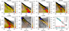 |
Fig. B.1 Average difference ( |
![Mathematical equation: $\[\bar{D}\]$](/articles/aa/full_html/2025/10/aa52590-24/aa52590-24-eq12.png)
![Mathematical equation: $\[\bar{D}_{\text {min}}\]$](/articles/aa/full_html/2025/10/aa52590-24/aa52590-24-eq13.png)
![Mathematical equation: $\[\bar{D}\]$](/articles/aa/full_html/2025/10/aa52590-24/aa52590-24-eq14.png)
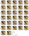 |
Fig. B.2 Same as Fig. B.1 but for PGCCs. The positions of minimum |
![Mathematical equation: $\[\bar{D}\]$](/articles/aa/full_html/2025/10/aa52590-24/aa52590-24-eq15.png)
![Mathematical equation: $\[\bar{D}_{\text {min}}\]$](/articles/aa/full_html/2025/10/aa52590-24/aa52590-24-eq16.png)
Best-fit gas densities and chemical ages for the objects.
All Tables
Molecular abundances observed in 32 PGCCs taken from Yi et al. (2018); Yi et al. (2021).
All Figures
|
Fig. 1 Comparison of |
| In the text | |
|
Fig. 2 Comparison between the best-fit chemical ages (black solid line; the formula labeled) and the ages from a modified free-fall collapse model with different B values for a 1 M⊙ cloud core (dotted, dashed, and dash-dotted lines). The gray region indicates an area twice that of the fit ages in order to cover the best-fit data points (black crosses) taken from Fig. B.1. The red vertical lines indicates a density of 7 × 104 cm−3. |
| In the text | |
|
Fig. 3 Abundance ratios (log[X(PAH)/X]) between the models with and without PAHs as a function of density. The ratios were calculated at the best-fit ages estimated through Eq. (B.1). The filled points, empty points, and crosses indicate the species in TMC-1 CP and L1544 that prefer the model with PAHs, prefer the model without PAHs, and have a non-detection in observations, respectively. The unfilled squares mark the species that are preferred by the models with and without PAHs. All the points with symbols except those with crosses indicate that the modeled abundances are within one order of magnitude of the observed ones. |
| In the text | |
|
Fig. 4 Abundance evolutionary tracks of PAH in the gas-phase (solid) and on the dust grain surface (dashed) in the cores with selected density (see legends with different colors). |
| In the text | |
|
Fig. 5 Same as Fig. 1 but for models with the low-metal (ℒ, upper panel) and high-metal (ℋ, upper panel) sets. The black and cyan colors indicate models without and with PAHs respectively. |
| In the text | |
|
Fig. 6 Fit linear correlation between log(t) and log(nH) using the models with the ℒ (dashed lines) and ℋ sets (dotted lines) without (black color) and with PAHs (cyan color). The solid black line shows the fit correlation of the models with the ℳ set (see Eq. (B.1)). The gray region indicates an area twice that of the fit ages as the same as that in Fig. 2. |
| In the text | |
|
Fig. 7 Fit correlation between the density and time (dashed line) using the reaction network from Sipilä et al. (2015). The solid line shows the fit result in Eq. (B.1). |
| In the text | |
|
Fig. 8 Cumulative probability of the ratio between the true and the beam-convolved parameters (N/Nconv, n/nconv and a/aconv) for the test cores with beams of 20 (left) and 40 arcsec (right). (See details in text.). |
| In the text | |
|
Fig. B.1 Average difference ( |
| In the text | |
|
Fig. B.2 Same as Fig. B.1 but for PGCCs. The positions of minimum |
| In the text | |
Current usage metrics show cumulative count of Article Views (full-text article views including HTML views, PDF and ePub downloads, according to the available data) and Abstracts Views on Vision4Press platform.
Data correspond to usage on the plateform after 2015. The current usage metrics is available 48-96 hours after online publication and is updated daily on week days.
Initial download of the metrics may take a while.