| Issue |
A&A
Volume 702, October 2025
|
|
|---|---|---|
| Article Number | A227 | |
| Number of page(s) | 10 | |
| Section | Planets, planetary systems, and small bodies | |
| DOI | https://doi.org/10.1051/0004-6361/202452779 | |
| Published online | 28 October 2025 | |
Extracting starspot structures from exoplanet transit photometry
1
Center for Astrophysics, University of Southern Queensland,
Toowoomba
4350,
Australia
2
Center for Radio Astronomy and Astrophysics, Mackenzie Presbyterian University,
Rua da Consolaçao, 896,
São Paulo,
Brazil
★ Corresponding author: This email address is being protected from spambots. You need JavaScript enabled to view it.
Received:
28
October
2025
Accepted:
6
September
2025
Abstract
Context. Future space-based transit photometry can provide empirical comparisons of solar and stellar spot structures with high precision. Spot transit mapping provides a way to directly observe and characterize the location, size, intensity, and evolution of starspots to infer stellar rotation rates and differential rotation.
Aims. We present a novel analysis technique to extend the scientific value of exoplanet transit mapping by extracting the umbral and penumbral structure of starspots from flux amplitude variations in transit light curves. We estimate the constraints on penumbral detectability according to transit depth, stellar brightness, and time-correlated and uncorrelated noise.
Methods. Our approach used simulated transits of a solar active region to determine the resulting flux ratios of occulted umbral and penumbral regions. The detection threshold of starspot penumbrae could be expressed in terms of flux variations in transit light curves, commensurate with penumbral intensities. We then examined the residual differences between noiseless and noise-added light curves for simulated transits of super-Earth and sub-Neptune sized exoplanets across spotted Sun-like stars. We used the PLATO Solar-like Light-curve Simulator to synthesize realistic photometric noise.
Results. We find that, under the right conditions, it is feasible to detect stellar umbrae and penumbrae with flux ratios matching solar values (1.4-4.2) in spotted transit light curves from the PLATO mission. The detection threshold was found to be a function of apparent stellar magnitude, as noise dominates for all but the brightest stars. In particular, penumbral flux variations can be distinguishable in the light curves of exoplanets as small as 3 R⊕ transiting the brightest Sun-like stars. Nevertheless, only the darkest penumbrae (0.66-0.70 Ic) are observed in the transit light curve of even the brightest 1 R⊙ star considered (mv = 8). However, for a 0.85 R⊙ star, the range of penumbral intensities is broader, at mv = 8 (0.66-0.85 Ic). A faint star limit of mv = 10 is found with only the darkest penumbrae (0.66-0.75 Ic) distinguishable, with penumbrae masked by the noise background for mv > 10.
Conclusions. High-precision transit photometry such as that from the PLATO mission can provide empirical comparisons of solar and stellar spot structures for an improved understanding of magnetic stellar activity and dynamo mechanisms.
Key words: sunspots / stars: activity / stars: solar-type / starspots
© The Authors 2025
 Open Access article, published by EDP Sciences, under the terms of the Creative Commons Attribution License (https://creativecommons.org/licenses/by/4.0), which permits unrestricted use, distribution, and reproduction in any medium, provided the original work is properly cited.
This article is published in open access under the Subscribe to Open model. This email address is being protected from spambots. You need JavaScript enabled to view it. to support open access publication.
1 Introduction
The surfaces of cool stars are known to exhibit different levels of magnetic activity. Indirect imaging techniques such as Doppler imaging, Zeeman-Doppler imaging, and eclipse mapping of binary systems have been used to chart magnetic structures on cool stars (Collier Cameron 1997; Savanov 2013). Photometric light curves of transited planet-hosting stars have been translated into maps of the stellar photosphere via spot modeling (Silva 2003). However, only active regions on the Sun have been observed directly. Images of the Sun provided by NASA’s Solar Data Observatory (SDO) show the distribution and polarity of magnetic regions and the heliographic location of active regions. Active regions on the Sun are temporally varying areas of intense magnetic fields that often contain subregions of inhibited convection of energy and heat from the solar interior, commonly known as sunspots.
Information gathered from direct observations of the Sun forms the basis for the understanding of processes active in cool solar-type stars. The projected surface activity of radiative-convective stars is extrapolated from decades of sunspot data. Long before G. E. Hale measured the magnetic fields of sunspots (Hale 1908), Galileo and his contemporaries in the 17th century noted that sunspots comprised a dark center, or umbra, surrounded by a shadow, or penumbra. In more recent times, astronomers have amassed a deeper understanding of these two regions, whose intensities differ relative to the unspotted stellar photosphere (Scharmer et al. 1985, 2002; Rouppe van der Voort et al. 2003). Time series of high-resolution images, such as those taken by the Swedish Vacuum Solar Telescope and the later Swedish 1-m Solar Telescope, have enhanced our knowledge of sunspot evolution and penumbral filamentary nature (Sánchez Almeida & Bonet 1998; Sobotka et al. 1999). Sunspots originate from dark pores that do not contain penumbrae. As a sunspot evolves, the umbra, or cool, dark core of a sunspot, is encased by a penumbra. The inner penumbra contains bright and dark filaments of varying intensities that radiate radially from the umbra, while the outer penumbra is bright and has a more consistent intensity (Sobotka et al. 1999; Li et al. 2018, 2022).
Sunspot structure infers magnetic complexity. The magnetic field lines within umbrae and penumbrae differ, with umbral fields being vertical and penumbral fields being horizontal relative to the solar surface (Jurcák et al. 2018). The gradation from umbra to penumbra is characterized by changes in magnetic field strength and intensity. The umbra contains a strong magnetic field and a corresponding constant intensity. The outer penumbra intensity is also constant but brighter than the umbra as a result of varying magnetic field strengths. The transition zone comprising the outer boundary of the umbra and the inner penumbra is marked by varying intensities with magnetic field strength less than that of the umbra. The boundaries between the different regions have also been described in terms of their intensities relative to the quiet solar photosphere (Mathew et al. 2007; Li et al. 2022, and references therein).
Nevertheless, the same processes that create umbrae and penumbrae on the Sun should also be at play in solar-type stars. The counterparts of sunspots, or starspots, have been observed on cool stars with a radiative-convective structure (Berdyugina 2004; Balona & Abedigamba 2016). Given the detail of available high-resolution spectropolarimetric and high-precision photometric data, we should theoretically be able to map starspot umbral-penumbral areas and intensities. To this point, Järvinen et al. (2018) presented the first evidence of a solar-like penumbra on EK Draconis, a young solar analog (≈50 Myr) with a rotation period of 2.6 d. They mapped the stellar surface temperature from ground-based, very high-resolution spectral data recorded by the Potsdam Echelle Polarimetric and Spectroscopic Instrument at the Large Binocular Telescope1 and reconstructed four spots, one of which is a large equatorial spot having unique umbral and penumbral temperature contrasts as compared to the quiescent photosphere. The spot diameter is ≈400 Mm, roughly 30 times the 13 Mm diameter of an average sunspot. Assuming a stellar effective temperature of 5730 K, the umbra and penumbra of that spot are 990 K and 180 K cooler, respectively. These differences were smaller than those for sunspots. Sunspot umbrae are 1000-1900 K cooler than the quiescent photosphere, while penumbrae are 250-400 K cooler (Solanki 2003).
Exoplanet transit light curves present another opportunity for indirectly measuring starspot structure and attributes. The Kepler mission (Borucki 2010) showed that high-precision photometry could not only reveal planets as small as Earth but also the spottedness of transited stellar surfaces (e.g., Désert et al. 2011; Sanchis-Ojeda & Winn 2011; Valio et al. 2017). The method of transits with small probing planets presents a favorable scenario for the identification of penumbral flux variations in the optical regime. We thus simulated transits across a solar active region to derive a penumbra to umbra flux ratio in ppm, which may be scaled for solar-type stars. This work is divided into the following major sections: In Sect. 2, we discuss the anatomy of an observed solar active region and present the results from simulated transits over that region. In Sect. 3, we introduce the transits of small exoplanets across solar-type stars for a parallel analysis. In Sect. 4, we present the results of simulated stellar transits followed by an evaluation of the impact of noise on penumbra detection with regard to the PLATO mission. In Sect. 5, we discuss the constraints to the detection of penumbrae posed by transit photometry. Finally, in Sect. 6, we present our conclusions and outlook.
2 Observing spots using transits
Transiting exoplanets are excellent probes of stellar surfaces. When a transiting planet occults a starspot or a starspot group, one or more bumps in a transit light curve are produced (Silva 2003). The width, height, and time of the center of the bump can be translated into individual starspot or starspot group radius, intensity, and longitude via modeling, for example, (Silva-Valio & Lanza 2011; Oshagh et al. 2013; Tregloan-Reed et al. 2013; Valio et al. 2017; Juvan et al. 2018; Zaleski et al. 2019, 2020; Netto & Valio 2020; Araújo & Valio 2021; Zaleski et al. 2022; Valio & Araújo 2022; Chakraborty et al. 2024).
Transiting hot Jupiters produce extremely deep transits in light curves and offer the broadest coverage of an active region. While optimal for discerning starspots in inherently noisy light curves, hot Jupiter transits make it difficult to distinguish between a starspot group and an individual spot or the fine detail of an individual starspot. The smaller the transiting exoplanet, the smaller the region of stellar disk occulted by the planet, and the higher the probability of observing fine starspot structure. The observing temporal cadence, or frequency of measurements, also has a significant effect on spatial resolution. Starspot signatures in transit light curves last on the order of minutes when an occulting exoplanet is in close orbit. Thus, a short observing temporal cadence is required to distinguish these features. To investigate the effects of exoplanet radius on observable active region detail and the ability to bound umbral and penumbral areas, we simulated the transits of Earth and super-Earth planets across a static image of the active Sun in October 2014 at short temporal cadences.
2.1 The transit model
Transit light curves for an exoplanet in a circular, non-oblique orbit were generated using the model ECLIPSE2 of Silva (2003). The model simulates a pixelated 2D white light image of a star with limb darkening, and computes the stellar intensity at each observation time interval as the sum of the intensities of planet-occulted and non-occulted pixels. The planet is represented as a dark, solid disk of specified radial size (relative to the stellar radius). The model can also use true solar images, white light, or other wavelengths (Selhorst et al. 2013). The orbit of the planet is calculated given the period, semimajor axis, a, and inclination angle, i. The transit latitude of the planet’s center is determined by the input stellar radius (R⋆), and orbital semimajor axis (a) and inclination angle (i), i.e., the inverse sign of the impact parameter as given by
![Mathematical equation: lat_{tr} = \arcsin \left[\frac{a \cos(i)}{R_{\star}}\right].](/articles/aa/full_html/2025/10/aa52779-24/aa52779-24-eq1.png) (1)
(1)
The dark disk of the planet (with zero intensity) is then “added” to the star image and positioned in the orbit for a given time. To produce the light curve, the intensity of all the pixels is computed for this instant in time, and then the planet is shifted to the next location, and again all the pixels intensities are summed, and so forth and so on. Finally, the light curve is normalized, where the out-of-transit intensity is set to unity.
Starspots can be added to the 2D stellar images at a given position (latitude and longitude), with a given intensity less than the disk center maximum intensity (Ic = 1). The occultation of active regions whose intensity is less than that of the quiescent photosphere results in bumps in the light curve due to reduced flux change. Thus, when the planet passes in front of a spot located in the transit band, a “bump” is detected for a short period of time as compared to the transit time. The model calculates the stellar longitude of the spot at this time interval, determined by the input observing cadence, according to
![Mathematical equation: lon_{tr} = \arcsin \left[\frac{a \cos \left(90^\circ - \frac{360^\circ\ t}{24\ P_{orb}}\right)}{\cos(lat_{tr})}\right],](/articles/aa/full_html/2025/10/aa52779-24/aa52779-24-eq2.png) (2)
(2)
where Porb is the orbital period, lattr is the transit latitude <90°, given in Eq. (1), and t is the observation time during transit.
Multiple spots at the transit latitude may be added to the stellar image. Spots may be monothermal or bithermal. An umbra and penumbra pair may be overlapped to create a complex spot. The intensity assigned indicates a darker umbral region, Ic ≤ 0.65, or a brighter penumbral region, 0.66 ≤ Ic < 1.0 (Li et al. 2022).
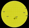 |
Fig. 1 Intensitygram of the Sun on October 23, 2014, at UTC 22:5 8:14.900, taken by the SDO HMI. AR12192 is the largest of the seven active regions, displaying sizable umbrae and penumbrae. |
2.2 Solar active region 12192 transits
Solar active region 12192 (AR12192), Hale Class βγδ, McIntosh Class Fkc), appeared in October 2014. It was the largest active region of Solar Cycle 24, reaching ≈2750 MSH3, equivalent to a circular area with the diameter of Jupiter. Fig. 1 is an intensitygram of the Sun taken on October 23, 2014, with the Solar Dynamics Observatory Helioseismic Magnetic Imager (SDO HMI) at UTC 22:58:14.900 and retrieved from the Joint Space Operations Center4 database. Unlike AR12194, which appears as a single spot, AR12192 contains multiple umbrae in a diffuse penumbral field.
Before transit simulation, the intensitygram was converted to a graticulated grayscale image, as shown in Fig. 2. The horizontal red lines highlight AR12192 in 2° increments of latitude for reference. Sunspot umbrae are dark gray to black, whereas penumbrae are medium gray. The umbra-penumbra boundary corresponds to an intensity of 148 on the pictured scale. Transits were simulated for latitudes −15°, −17°, and −21°, at which there are distinct circular umbral regions with adjacent penumbrae. Latitude −19° was not selected due to the diffuse umbral structure between −2° and 1° of longitude. Blue circles representing 1, 1.5, and 2 R⊕ super-Earth planets in Fig. 2 highlight the relative sizes of the starspots at the chosen latitudes.
In order to capture the in-transit variations due to occulted umbrae and penumbrae, we simulated the transits of Earth-sized planets orbiting the Sun. The cataloged exoplanet population contains some 160 Earth-sized planets transiting solar-type stars whose radii are within ±5% of 1 R⊕5. We thus chose a representative orbital semimajor axis of 0.06 au. In accordance with Kepler’s third law, the planetary orbital period is 5.362 d. The transit duration at the aforementioned solar latitudes is ≈3.4 h. All transits are considered to be noiseless in that they are unaffected by time-variant noise. The static solar image incorporates minimal photon noise equal to 0.01% of the intensitygram measurements (Couvidat et al. 2016). Thus, the transits yield idealized, noise-free amplitudes for umbra and penumbra crossings.
Lastly, we considered the observational temporal cadence for our simulations. The granularity of flux amplitude variations depends on temporal cadence, improving as the time interval shortens. With an eye on the upcoming PLATO mission, we chose an observational cadence of 25 s. The PLATO mission will employ 24 small aperture telescopes to record white light data at a 25 s read-out cadence and two additional telescopes equipped with red and blue filters for capturing bi-spectral images every 2.5 s (Rauer et al. 2014, 2016, 2025). We also suggest that knowledge acquired from a baseline of in-transit amplitude variations due to magnetically active regions at the PLATO temporal cadence (25 s) can be applied to the analysis of TESS light curves with a slightly higher cadence (20 s) (Ricker et al. 2014; Jenkins et al. 2021).
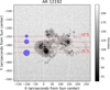 |
Fig. 2 Graticulated grayscale enlargement of AR12192. The red lines mark the latitude in 2° increments, while the blue circles represent planets with sizes of 1, 1.5, and 2 R⊕ and highlight the relative sizes of the planets and the spots. |
2.3 Decoding sunspot structure
Baseline light curves for a 25 s observing cadence were generated for super-Earths transiting the white light image of the Sun on October 23, 2014 (see Fig. 2). Orbital inclinations of 88.85°, 88.70°, and 88.40° prescribed the transit latitudes of −15°, −17°, and −21°. The transit light curves for 1 R⊕, 1.5 R⊕, 1.8 R⊕, and 2 R⊕ planets are shown in Fig. 3. These planetary radii were chosen to best demonstrate the effect of exoplanet radial size on penumbra observability. The orbits for all planets were circular with a 5.362 d period at a distance of 0.06 au from the Sun for comparison purposes. At all transit latitudes, the light curves for a 2 R⊕ planet show bumps that are recognizable as spots. The −15° and −21° light curves each have 2 bumps, while the −17° transit has a third bump at ≈-0.85 h transit due to the occultation of AR12194.
As the planet’s radial size is reduced, transit depth along with bump height decreases as a result of the coverage of smaller and smaller areas on the stellar surface along the transit chord, while the relative scaling of the two is maintained. However, the key result of decreasing planet size is reduced umbra-penumbra blending that can reveal flux variations due to spot substructures. The sunspots near mid-transit in the light curves for a 1 R⊕-sized planetary transit exhibit asymmetries, which we attribute to umbral and penumbral crossings. Active regions that were generically identified as spots are now separated into umbrae and penumbrae. The light blue and orange arrows in Fig. 3 point to the umbrae and penumbrae, respectively. Penumbrae are expressed as sharp or rounded shoulders adjacent to umbral peaks. The irregular shape, or horizontal extent, of the penumbral field surrounding an umbra dictates whether a penumbral shoulder is observed to the left and/or right of an umbral peak. In the grayscale image of the Sun (Fig. 2), the penumbral area encasing the large umbra at −21° is horizontally wider to the left of the umbra than to its right. This is reflected in the transit light curve for a 1 R⊕ planet as a peak at mid-transit having shoulders of similar intensity but different widths. At the other transit latitudes, the umbrae lie closer to an outside boundary of their neighboring penumbrae and, thus, appear as peaks with a single shoulder in the light curves. At the −15° transit latitude, for example, the peak at approximately +0.04 h corresponds to a relatively small umbra at longitude 1.5°, while the penumbra appears as shoulder at 0.12 h, or longitude 4.5°.
Penumbral shoulders smooth as the size of the transiting exoplanet increases, some eventually blending into the umbrae to form generic big bumps. As may be noted by the red curves in Fig. 3, blending becomes significant at 1.8 R⊕. Beyond this cutoff radius, penumbral shoulders are, for all practical purposes, indistinguishable.
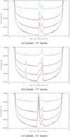 |
Fig. 3 Simulated light curves for 1 R⊕ (green), 1.5 R⊕ (blue), 1.8 R⊕ (red), and 2 R⊕ (black) planets transiting the October 23, 2014 Sun at latitudes −15° (a), −17° (b), and −21° (c). The orbital period and semimajor axis are 5.362 d and 0.06 au, respectively, and the observing cadence is 25 sec. The light blue and orange arrows point to the umbrae and penumbrae, respectively. |
Umbrae and penumbrae longitudes and flux residuals.
2.4 Umbra-penumbra flux ratio
To measure the flux variations induced by umbra and penumbra crossings, we considered the transits of the 1 R⊕ planet across AR12192. Normalized flux residuals for each latitude were calculated by subtracting the model light curve for the transit of a 1 R⊕ planet across an unspotted Sun (as described in Sect. 2.1) from the spotted light curves. A grayscale image of the unspotted Sun was created by masking AR12192. Umbrae and penumbrae were identified by comparison with the grayscale SDO image of the Sun on October 23, 2014. The residuals for the umbral-penumbral regions of interest are summarized in Table 1 with commentary. Also included in that table are the transit times of the umbrae and/or penumbrae and their equivalent longitudes converted from the transit time at the transit latitude using Equation (2).
We calculated the umbra-penumbra flux ratios (Fu/Fp) from the normalized flux residuals in Table 1 for the two umbrapenumbra pairs at latitude −15°, the umbra-penumbra pair at latitude −17° and the penumbra-umbra-penumbra at latitude −21°. As listed in Table 2, the minimum value of Fu/Fp is 1.4 at latitudes −15° and −17°. The maximum value of Fu/Fp is 4.2 at latitude −21°, where the umbral contrast, or flux variation, is the greatest.
Flux ratios of umbra-penumbra pairs.
2.5 Reconstructing AR12192
We modeled the umbrae and penumbrae listed in Table 1 for the 1 R⊕ planetary transits to estimate their radial widths, intensities, and longitudes. To this end, we employed an IDL6 version of emcee (Foreman-Mackey et al. 2013), originally a Python implementation of the Markov chain Monte Carlo (MCMC) ensemble sampler proposed by Goodman & Weare (2010). For each transit latitude, parameter estimation was performed simultaneously with ECLIPSE as the generative model for a combination of four substructures (umbrae and penumbrae), as appropriate at the transit latitude. The stellar image in the pixelated stellar grid used in the ECLIPSE function had a user-defined radius of ≈413 pixels, which corresponds to a resolution of 4.59 pixels per degree, or about 0.22 degrees per pixel. This resolution was sufficient for the retrieval of starspot substructures.
The uniform priors defined a broad parameter space delimited by longitude from −70° to 70°, radius from 0.02 to 10.0 times the planet radius, and intensity from 0.01 to 0.65 Ic for umbrae and 0.66 to 0.945 Ic for penumbrae. Tens of thousands of walker moves sampled the parameter space with the initial guesses in a tight ball approximating the parameter values in the neighborhood of maximum probability. The resulting most likely parameter values and their 1σ uncertainties are summarized in Table 3.
The stellar surface at the transit latitudes as reconstructed using the most probable parameters is shown in Fig. 4a. A grayscale image of AR12192 that covers the same boundaries as the reconstructed region is juxtaposed in Fig. 4b. The intensity scale is the same as that shown in Fig. 2. Comparison between the reconstructed and original images of AR12192 shows that while the very fine detail of the active region is not reproducible, we captured the essence of that active region. The resolution used in this work (≈9 pixels per 2 degrees) represents a compromise between spatial resolution and computational cost and has minimal effect on the substructures in the reconstructed image, since their intensities are uniform.
3 From sunspots to starspots
If starspots on solar analogs replicate the structure of sunspots, then we propose that the flux amplitude variations seen in the transit light curves of those stars should infer equivalent sunspot flux ratios, i.e., Fu/Fp from 1.4 to 4.2, regardless of starspot radial size. Sunspot sizes follow a log-normal distribution (Valio et al. 2020) and are generally considered to be small (Solanki & Unruh 2004). The radii of most sunspots range from 13 to 25 × 103 km and can be as large as 40 or 50 × 103 km. The penumbra-umbra area ratio is ≈4.5 for small sunspots and 5.5-6 for large spots (Jha et al. 2019), inferring that the penumbrae size can be some 2 times that of the umbrae.
Stars in the Kepler database with Sun-like rotation periods and temperatures have smaller spots than spectral type mid-G and cooler stars (Giles et al. 2017). Transit mapping studies of solar-type stars that are cooler and rotate faster than the Sun yield large spots. Starspots on Kepler-71 (G7V, rotation period 19.77 d, 0.887 R⊙) have a mean radius of (51 ± 26) × 103 km and a maximum radius of 138 × 103 km (Zaleski et al. 2019). Another G7V star, CoRoT-2 (rotation period 4.52 d, 0.902 R⊙), also has large spots ranging in size from 40 × 103 km to 150 × 103 km (Wolter et al. 2009). Similarly, the mean radius of starspots on KOI-883 (K2V, rotation period 8.99 d, 0.69 R⊙) is (57 ± 26) × 103 km with a maximum radius of 121 × 103 km (Zaleski et al. 2022). For Kepler-45 (M1V, rotation period 15.76 d, 0.624 R⊙), the mean starspot radius is (40 ± 17) × 103 km, with a maximum radius of 78 × 103 km (Zaleski et al. 2020). The mean radius of starspots on Kepler-17 (G2V, rotation period 12.4 d, 1.05 R⊙) is (49 ± 10) × 103 km (Valio et al. 2017) and on the young G-type star Kepler-63 (rotation period 5.4 d, 0.938 R⊙) is (33 ± 12) × 103 km (Netto & Valio 2020). The given stars are all transited by hot Jupiters. Their planet-to-star radius ratios are 0.136, 0.163, 0.184, 0.182, 0.138, and 0.066, respectively, producing deep transits with a high signal-to-noise ratio (S/N).
While well suited to observing starspots, the transits of these five exoplanets did not reveal umbra-penumbra detail due to their radial sizes relative to their host stars. Flux variations indicative of broad penumbrae for the largest starspots were not evident. As mentioned earlier, the smaller the planet size, or the probe, the more detail can be observed on the transit light curve of spots, or other features on the surface of stars. As the planet size increases, the individual spots of an active region, or the even less pronounced fine structure within a spot, cannot be distinguished.
The capture of starspot structural detail requires that the transiting planet be small, for example, a super-Earth (1 to ≤2 R⊕) or sub-Neptune (>2 to ≤4 R⊕). Such an occulting body will probe a shallower cross section of the stellar face and yield a light curve with a transit depth less than that of a larger planet. However, it remains possible to record finer flux variations at a high observation cadence. Yet, as the planet size decreases, so does the transit depth, and the spot signatures become more and more contaminated by the noise of the observation. That is the case of the Kepler-411 (Araújo & Valio 2021) and Kepler-210 (Valio & Araújo 2022) systems with small planets for which the data are noisy, and it is not possible to distinguish penumbrae in the spots’ signatures.
MCMC umbra and penumbra parameters.
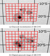 |
Fig. 4 Grayscale images of AR12192 as (a) reconstructed from the Bayesian parameter estimation for the simulated transits at latitudes −15°, −17°, and −21° and (b) extracted from the SDO HMI intensitygram. The gridded region covers latitudes −10° to −24° and longitudes −8° to −12° in 2° increments. |
4 Simulated transits of PLATO stars
Under the assumption that large starspots have sizable umbral and penumbral regions, they are excellent targets for morphological studies. The larger the starspot relative to the radial size of the probing exoplanet, the higher the probability of acquiring flux variations indicative of both umbrae and penumbrae. Transit light curves from the much anticipated PLATO mission are of particular importance for the study of starspots since the telescope will observe solar-type stars over an extended period of time while recording the transits of Earth-sized planets at an observational cadence of 25 s. Data for dwarf stars of spectral types F5-K7 will be collected in three stellar samples at different V-band apparent magnitude limits (11, 8.5, and 13). A fourth stellar sample will be dedicated to M dwarfs of apparent magnitude ≤16 (Montalto et al. 2021; Rauer et al. 2025).
The transit light curves of active stars in the PLATO sample will be modulated by starspots, and flux amplitude variations due to any starspots coincident with the transit chord will be captured. The ability to separate starspots into umbrae and penumbrae will largely be determined by the S/N relative to the transit depth. The predominant noise sources that affect transit light curves include photon noise, random noise, pressure mode (p-mode) oscillations, and stellar granulation. The oscillation and granulation patterns of the Sun have been investigated by Chiavassa et al. (2017) and Morris et al. (2020) using static solar images. Sulis et al. (2020) and Krenn et al. (2024) have performed similar studies by modeling an exoplanet transit across a series of time-variant solar images. In order to evaluate the cumulative effect of time-dependent and stochastic noise on the recovery of in-transit starspot data, we chose the publicly available PLATO Solar-like Light curve Simulator (PSLS)7 to synthesize realistic, time-variant uncertainties affecting transit light curves for spotted Sun-like stars (Samadi et al. 2019).
4.1 PLATO Solar-like Light curve Simulator (PSLS)
The PSLS models the total of time-correlated and uncorrelated noise characteristic of main sequence, subgiant, and red-giant stars of different apparent stellar magnitudes. At each cadence (default = 25 s), the flux variation in ppm for each camera is calculated from the sum of stellar activity, residual systematic error, random error, and stellar oscillations and granulation matching those of previously observed stars. The flux variation profiles per camera can be averaged over a user-specified number of cameras.
The oscillation spectrum for a main sequence star is generated based on pulsations models from the Aarhus Adiabatic Pulsation (ADIPLS) code (Christensen-Dalsgaard 2008) or stellar evolution code CESAM2K (Code d’Evolution Stellaire Adap-tif et Modulaire) (Morel 1997; Morel & Lebreton 2008). The granulation background is modeled as a single Lorentzian component or as two pseudo-Lorentzian profiles with different line heights, characteristic timescales, and slopes according to the scaling relations prescribed by Kallinger et al. (2014). The stellar activity is also simulated using a Lorentzian profile, but the user must provide the amplitude and the timescale.
In addition to the stellar phenomena that affect the disk-integrated flux intensity, PSLS accounts for the level of instrumental noise (systematic and random) including shotnoise, read-out noise, and satellite jitter. The PSLS distribution includes tables of systematics at beginning of life (BOL) and end of life (BOL) conditions.
A transit light curve may be superimposed on the background described above following the equations of Mandel & Algol (2002). The physical characteristics of the planet and its orbit are radius, semimajor axis, orbital period, and orbital angle. The limb darkening coefficients of the star must also be provided. The value computed by PSLS at each cadence is the sum of light curve flux and noise.
Lastly, spots may be added to the stellar surface at any latitude and longitude using the circular spot model of Dorren (1987). Spots are described by their radii, single-value contrasts relative to the photosphere, and lifetimes. As with the addition of a transit light curve, the presence of spots affects only the flux per observational cadence and not the global oscillations. This feature enables the synthesis of light curves for the analysis of starspot characteristics in the Fourier domain, where photometric degeneracies are reduced (Degott et al. 2025). However, these light curves are not suitable for the study of complex occulted starspots.
The PSLS models global oscillations and does not address dampening of p-mode oscillations in active regions. The amplitude of pressure mode oscillations differs between the quiet, non-magnetically active photosphere and magnetically active regions (Jain & Steele 2007, and references therein). Pressure mode oscillations excited by surface convection are not dampened in the non-magnetically active photosphere, while the intense magnetic fields within spots alter the excitation properties of turbulent convective motion and effect reductions in wave oscillation amplitude (Parchevsky & Kosovichev 2007; Kosovichev 2009). Wave properties within umbral and penumbral substructures further differ due to the organization of magnetic field lines and strengths. In umbrae, magnetic field lines are largely vertical, and the magnetic field is strongest; while in penumbrae, magnetic field lines are highly inclined and the magnetic field is weaker than that of the umbra. When a p-mode wave crosses the quiet photosphere-penumbra boundary, the magnetic field within the penumbra causes the wave frequency to be shifted and the amplitude to be dampened as the wave travels to the umbra-penumbra boundary. Wave amplitude reaches a minimum in the umbra as 5 min oscillations are converted into magnetohydrodynamic waves at different eigenmodes under the forces of magnetic tension and magnetic pressure (Cally et al. 2003; Zhao et al. 2011; Stangalini et al. 2020). In the uniform umbra, the reduction in amplitude of incoming p-mode waves is estimated to be some 50% (Parchevsky & Kosovichev 2007). To date, there is no prescription for modeling local oscillations in starspots. Reduction of the noise due to oscillations may enhance penumbral signatures.
4.2 Transits of spotted Sun-like stars
4.2.1 Data and method
Our approach to simulating the transits of spotted Sun-like stars was multistep. We first employed PSLS to generate realistic noise backgrounds for transited Sun-like stars having different radii over a range of apparent stellar magnitudes (mv = 8-12). Since PSLS treats the overall noise and light curve flux variations independently prior to summing them, a spot was not added to the stellar face. We, instead, extracted the noise background and then applied it to noiseless spotted transits simulated via ECLIPSE.
Sun-like stars having different radii were chosen in order to investigate the impact of background noise and transit depth on the observability of starspot substructures. We selected two stars from the grid of CESAM2K stellar models, one resembling the Sun and the smallest Sun-like star in the grid. The stars have the following fundamental parameters: Star 1-1 R⊙, 0.98 M⊙, Teff = 5706 K, and log g = 4.43; Star 2 - 0.85 R⊙, 0.95 M⊙, Teff = 5751 K, and log g = 4.56.
Configuration files (Yet Another Markup Language (YAML) files) input to PSLS prescribed the simulation of transit light curves spanning 10 d for 1, 2, and 3 R⊙ planets orbiting Stars 1 and 2 at a cadence of 25 s for all 24 cameras at BOL. Solar limb darkening was applied to the stellar photospheres, a simplification having minimal impact on the shape of the transit wells and facilitating comparison of the simulated light curves. As in the solar simulations, the planets’ orbital period and semimajor axis were 5.362 d and 0.06 au. The orbital inclination relative to the stellar rotation axis was 90°. The observation window was set to 10 d. Unique configuration files were created for apparent stellar magnitudes 8-12 in integral steps for each star-planet combination. Upon execution of a YAML file, PSLS automatically saved the simulated noisy light curve representing an average of 24 light curves corresponding to the number of cameras.
The noise backgrounds were subsequently separated into out-of-transit and in-transit datapoints. We calculated the rms of the out-of-transit noise for later comparison with penumbral flux variations. Table 4 lists unsmoothed (25 s) and three-point smoothed (75 s) 1σ values. The unsmoothed 1σ values are the averaged rms noise derived from multiple iterations of configuration files at a given apparent stellar magnitude. Individual rms values differed by ≈1%.
Noiseless spotted transit light curves for the six star-planet pairs were generated with ECLIPSE using the same physical parameters input to PSLS. A sizable bithermal spot was superimposed at the center of a white light stellar image with solar limb darkening (coefficient u = 0.65) (Moon et al. 2017). The total radial extent of the starspot was 46 × 103 km, representative of the starspots estimated for the aforementioned Kepler stars and ≈8% larger than the reconstructed spot at latitude −21° in AR12192. The radius of the umbra was 23 × 103 km, half that of the penumbra. The centers of the umbra and penumbra were located at 0° and −2° stellar longitude along the transit latitude in the observer’s frame, sufficient to produce an umbral shoulder in the light curves. The longitudinal offset mimics the appearance of solar umbrae and penumbrae in Fig. 2. For each iteration of ECLIPSE, the intensity of the umbra was 0.1 Ic. The intensity of the penumbra was first set at 0.66 Ic and could thereafter vary from 0.70 to 0.90 Ic in increments of 0.05. The magnitudedependent noise flux extracted from the PSLS output files was then added to candidate, noiseless spotted transits by temporally matching the PSLS and ECLIPSE datapoints relative to mid-transit (h = 0). The residuals resulting from the subtraction of the noiseless light curves from the noise-added light curves were 3-point smoothed, and the penumbral flux variations were compared to 3 × σ75s values.
PSLS noise background vs. apparent stellar magnitude.
4.2.2 Results
Following the procedure described in the previous section, we evaluated the relationship between penumbra-induced flux amplitude variations and the noise level of simulated PLATO transit light curves. Six sets of transit light curves were synthesized for Earth-, super-Earth-, and sub-Neptune-sized exoplanets occulting a large complex spot at the centers of Stars 1 and 2. For each planet-star combination, we considered the penumbral contrast with the unspotted photosphere (Ic = 1) as a function of the apparent stellar magnitude. The apparent stellar magnitude, mv, determines the level of simulated light curve noise and, thereby, the minimum and maximum intensities (i.e., the greatest and lowest contrasts) of the penumbrae producing detectable flux variations. For detection, the flux residuals of observable penumbrae have to be greater than three times the smoothed rms of the out-of-transit noise background for a star at a given apparent magnitude.
As expected, the transits of a 1 or 2 R⊕ exoplanet across a 0.85 or 1 R⊙ star are not deep enough to allow the detection of penumbra even for the brightest stars and darkest penumbrae. The flux variation due to a penumbra with intensity 0.66 Ic in the noiseless spotted light curve for the deeper transit of the 2 R⊕ exoplanet across a 0.85 R⊙ star is ≈ 185 ppm, less than the 3 × σ75s benchmark for mv = 8. Penumbra detection was thus limited to the deeper transits of a 3 R⊕ planet.
Within the combinations of stellar radius, penumbral intensity, and apparent stellar magnitude with a fixed planetary radius of 3 R⊕, we found cases for which the residual penumbral flux exceeded the σ75s rms of the PSLS out-of-transit noise background. The plots in Fig. 5 present the residuals for four representative cases and exemplify the constraints imposed by noise and transit depth on extracting penumbral signatures in the transits of sub-Neptune-sized planets. In all plots, unsmoothed residuals are represented by a black, irregular curve with an overlay in red after three-point smoothing. A horizontal blue line indicates the 3σ noise level, and a vertical green line marks the umbra-penumbra boundary. The curves span ±1 h from mid-transit, focusing on the residuals of the complex spot.
As shown in Fig. 5a for a 3 R⊕ exoplanet occulting the large spot on a bright 1 R⊙ star (mv = 8), the shoulder of a dark penumbra (Ic = 0.70) lies just above the 3σ noise level. Thus, only penumbrae with the highest contrast, i.e., Ic = 0.66 (not shown) and 0.70, may be detectable. The flux variations of the penumbrae at these intensities are 280 and 250 ppm, respectively, with corresponding values of Fu/Fp being 3.6 and 3.2 for an umbral flux height of 900 ppm. The range of observable penumbral intensities broadens as the transit depth increases, and the apparent stellar magnitude is kept constant. The noise level relative to the penumbral flux variation is reduced. When the planet occults the same spot on the smaller 0.85 R⊙ star, the maximum penumbral intensity is 0.85 Ic (see Fig. 5b). The variation in penumbral flux is 300 ppm, with Fu/Fp = 3.7.
The plots in Figs. 5c and 5d further demonstrate the dependence of penumbra detectability on noise as a function of apparent stellar magnitude for a Sun-like star smaller than the Sun. As the star dims, the contrast of the observable penumbrae with the surrounding photosphere lessens. We found that the observable penumbral intensity decreases by 0.05 for each order-of-magnitude reduction in stellar brightness from mv = 8 to 10. At mV = 10, the penumbral intensity is not greater than 0.75 Ic, while it is as bright as 0.85 Ic at mV = 8. The darker and cooler the penumbra, the greater its impact on the transit light curve. Consequently, the variation of the penumbral flux decreases from 600 to 300 ppm with reduced photospheric contrast, and Fu /Fp increases from 2.1 to 3.7 relative to an umbral intensity of 0.1 Ic. These ratios approximate solar values, as expected. For stars at mV ≥ 11, the penumbrae of all intensities are masked by noise.
Table 5 summarizes the limits to the penumbra photometric visibility with respect to the PSLS simulated noise for PLATO transit light curves for all planet-star scenarios addressed in this work. The value of penumbral intensity is within 0.66 Ic for the darkest, most contrasting penumbra to 0.85 Ic for the brightest, least contrasting penumbrae. The table lists the intensity of the brightest penumbra hypothetically observable for occulted starspots relative to apparent stellar magnitude.
5 Discussion
Important constraints to penumbra detection can be inferred for the PLATO mission from Table 5. First, the intensity of observable penumbrae decreases (i.e., darkens) as stellar magnitude and noise background increase. The dimmer the star, the darker and cooler the observable penumbra has to be. Penumbrae with lower photospheric contrast will be visible on brighter stars, whereas only the darkest penumbrae will be visible on dimmer stars. For example, in the case of a 3 R⊕ planet transiting a 0.85 R⊙ star, the maximum penumbral intensity (lowest contrast) is 0.85 Ic for mv = 8, decreasing to an intensity of 0.75 Ic at mv = 10.
Second, the stellar brightness at which penumbrae may be detected is strongly dependent on transit depth. Penumbra detection requires transit light curves with a high S/N. The fainter the star, the deeper the transit needs to be. For instance, the transit depth of a 3 R⊕ planet crossing a 0.85 R⊙ star is ≈1050, whereas the noise level (three times the 75 s rms) is ≈910 and 1600 ppm at mv =11 and 12, respectively. Thus, penumbrae will not be observed for apparent stellar magnitude of the host star of ≥10. Detection of starspot penumbrae on Sun-like stars in the PLATO light curves will be limited to only the brightest stars smaller than the Sun.
These constraints may still be compatible with the PLATO mission objective to observe small planets orbiting M dwarf stars of mv < 14 and bright K-type stars (mV ≤ 11). We propose that the observability of penumbrae with decreasing contrast relative to the stellar photosphere will improve with increasing planet-star radius ratio. However, while the radius of an occulting planet in relation to the radial extent of a penumbra dictates the shape of the penumbra’s signature in a transit light curve, the width of a penumbral shoulder does not guarantee detectability, which is primarily governed by the penumbra’s intensity in terms of its corresponding flux amplitude.
In our simulated light curves, a shoulder lasting ≈3 min was created by separating the centers of the umbra and the penumbra by 2° for the purpose of assessing its visibility as a function of apparent stellar magnitude. The results would have been identical for a larger complex spot. We anticipate that the continuous monitoring of the PLATO mission will yield long duration spot crossings for small planets in long-period orbits about active stars, possibly enabling the detection of temporally broader penumbral shoulders.
The replication of AR12192 from spot physical parameters estimated by MCMC fits to simulated light curves indicates that it is possible to reconstruct active regions along a transit chord. If and when flux amplitudes due to umbrae and penumbrae are found in the high-precision PLATO transit light curves of target stars, detailed pictures of active regions will be built.
The method of transits presents the first opportunity to identify penumbral flux variations in the optical regime. Earlier research considered the difference between umbrae and penumbrae in terms of their intensities in images at different wavelengths, such as the infrared (Maltby 1972; Ekmann 1974). Based on our knowledge of sunspots and on the simulations in this work, it is hypothetically feasible to distinguish starspot umbrae and penumbrae in the transit light curves of bright stars smaller than the Sun. Transit detection efficiency, as determined by exoplanet radial size, i.e., transit depth, and light curve noise level, directly affects the ability to observe active regions occulted during transit and further limits the morphological dissection of active regions (Pont et al. 2006). Starspot analysis requires a high S/N that is not degraded by contributions of photon noise and stellar variability among other factors (Taaki et al. 2020).
Photometric precision is particularly critical for the transits of small planets with shallow transits (Tregloan-Reed et al. 2013). Depending on a star’s magnitude and activity level, stellar variability can cause significant, erratic flux changes and high rms values both in- and out-of-transit that hamper photometric analysis. The Kepler mission, for example, had an average combined differential photometric precision (CDPP) of 30 ppm. The sensitivity of TESS is lower with a CDPP of 100 ppm mainly due to the use of smaller lenses (Battley et al. 2021). The PLATO mission proposes a 34 ppm precision over 1 hour integration for stars with magnitude <11 increasing to 80 ppm for 13th magnitude (Rauer et al. 2014) and a detection efficiency of 100% for Earth analogs to giant-sized planets. For the faintest M dwarfs, the precision degrades to 800 ppm. These values are promising, but still imply that penumbra detection be limited to relatively shallow transits in the highest quality data.
Observing temporal cadence must also be considered when evaluating starspot structure. Starspot signatures last for a few minutes, whereas transit durations scale with hours. For example, starspots are not evident in Kepler long cadence light curves while they are in short cadence light curves (Zaleski et al. 2019). The TESS mission postage stamp light curves at 20 s cadence offer a current resource for investigating starspot structure. The upcoming PLATO mission will observe stars down to V-magnitude 16 with a normal read-out cadence of 25 s, enabling better temporal resolution of spot structures. As its predecessor Kepler, PLATO will undertake long-term continuous monitoring of stellar fields. Improved photometric efficiency with a low noise-to-signal ratio is a key goal of the mission.
Noise from sources such as p-mode oscillations and granulation may be averaged out via binning on timescales longer than starspot temporal signatures (Oshagh 2018). Such binning will also remove starspots. Gaussian process regression is a more computationally intensive technique for modeling stellar variability to improve the characterization of transit parameters. Gaussian processes perform well in detrending light curves for transit retrieval. However, there remains the need to preserve starspots while lessening the variability, which confounds umbra and penumbra detail. Future noise reduction algorithms may more effectively address the removal of variability.
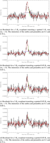 |
Fig. 5 Residuals (black) from the subtraction of noiseless, spotted transit light curves from noise-added, spotted light curves for four combinations of stellar radius, planetary radius, and stellar apparent magnitude. Red curves represent the residuals after three-point smoothing. Horizontal blue lines are the 3 × σ75s noise level, while vertical green lines mark the umbra-penumbra boundaries. Detectable penumbral have residuals above 3 × σ75 s. |
Maximum intensity of observable penumbra above PLATO noise vs. planet-star radii and stellar magnitude.
6 Conclusions
We present evidence that, under optimal conditions, transit photometry can reveal the two-component structure of starspots, namely, dark umbrae surrounded by larger, brighter penumbrae. Our simulations of Earth-, super-Earth-, and sub-Neptune-sized planets transiting solar-type stars suggest that the resulting flux variations between umbrae and penumbrae are consistent with values observed in solar analogs. This technique offers a method for distinguishing between umbral and penumbral regions on other stars. However, its effectiveness depends strongly on the S/N, the contrast of the penumbra with the stellar photosphere, the cadence of observations, and the overall brightness of the host star.
In general terms, the results suggest a way forward to advance beyond existing studies that map large-scale starspots on the most active cool stars. Our study opens the possibility to systematically survey Sun-like spot features, which are expected from dynamo theory to be common and cyclic. This would provide new insights into stellar dynamos, although it is yet a challenge to those seeking to disentangle stellar activity from intrinsic exoplanet properties.
We thus recommend that suitably precise and extensive exoplanet transit photometry, in combination with noise reduction algorithms, be considered as a way to further compare solar and stellar spot structures in the future. Such investigations will rely on the best available photometry from next-generation telescopes in space (such as PLATO), or from major ground-based facilities if similar precision can be obtained. Such studies of stellar activity and hence stellar dynamos can then be added to the science cases for planned or proposed exoplanet photometry projects.
Acknowledgements
The authors thank the anonymous referee for comments and suggestions that improved the results. The authors also thank Réza Samadi for sharing the grid of CESAM2K stellar models. AV acknowledges partial financial support from Brazilian FAPESP agency (#2018/04055-8 and #2021/02120-0).
References
- Araújo, A., & Valio, A. 2021, ApJ, 922, 23 [NASA ADS] [CrossRef] [Google Scholar]
- Balona, L. A., & Abedigamba, O. P. 2016, MNRAS, 461, 497 [NASA ADS] [CrossRef] [Google Scholar]
- Battley, M. P., Kunimoto, M., Armstrong, D. J., et al. 2021, MNRAS, 503, 4092 [CrossRef] [Google Scholar]
- Berdyugina, S. V. 2004, Sol. Phys., 224, 123 [Google Scholar]
- Borucki, W. J. 2010, Science, 327, 977 [CrossRef] [PubMed] [Google Scholar]
- Cally, P. S., Crouch, A. D., & Braun, D. C. 2003, MNRAS, 346, 381 [Google Scholar]
- Chakraborty, H., Lendl, M., Akinsanmi, B., Petit dit de la Roche, D. J. M., & Deline, A. 2024, A&A, 685, A173 [NASA ADS] [CrossRef] [EDP Sciences] [Google Scholar]
- Chiavassa, A., Caldas, A., Selsis, F., et al. 2017, A&A, 597, A94 [NASA ADS] [CrossRef] [EDP Sciences] [Google Scholar]
- Christensen-Dalsgaard, J. 2008, Ap&SS, 316, 113 [Google Scholar]
- Collier Cameron, A. 1997, MNRAS, 287, 556 [NASA ADS] [CrossRef] [Google Scholar]
- Couvidat, S., Schou, J., Hoeksema, J. T., et al. 2016, Sol. Phys., 291, 1887 [Google Scholar]
- Degott, L., Baudin, F., Samadi, R., Perri, B., & Pincon, C. 2025, A&A, 696, A41 [NASA ADS] [CrossRef] [EDP Sciences] [Google Scholar]
- Désert, J.-M., Charbonneau, D., Demory, B.-O., et al. 2011, ApJS, 197, 14 [Google Scholar]
- Dorren, J. D. 1987, ApJ, 320, 756 [Google Scholar]
- Ekmann, G. 1974, Sol. Phys., 38, 73 [Google Scholar]
- Foreman-Mackey, D., Hogg, D., Lang, D., & Goodman, J. 2013, PASP, 125, 306 [NASA ADS] [CrossRef] [Google Scholar]
- Giles, H. A. C., Collier Cameron, A., & Haywood, R. D. 2017, MNRAS, 472, 1618 [Google Scholar]
- Goodman, J., & Weare, J. 2010, Commun. Appl. Math. Computat. Sci., 5, 68 [Google Scholar]
- Hale, G. E. 1908, ApJ, 28, 315 [Google Scholar]
- Jain, R., & Steele, C. D. C. 2007, A&A, 473, 937 [NASA ADS] [CrossRef] [EDP Sciences] [Google Scholar]
- Järvinen, S. P., Strassmeier, K. G., Carroll, T. A., Ilyin, I., & Weber, M. 2018, A&A, 620, A162 [NASA ADS] [CrossRef] [EDP Sciences] [Google Scholar]
- Jenkins, J. M., Twicken, J. D., Tenenbaum, P. G., et al. 2021, in AAS Meeting Abstracts, 53, 134.01 [Google Scholar]
- Jha, B. K., Mandal, S., & Banerjee, D. 2019, Sol. Phys., 294, 72 [Google Scholar]
- Jurcák, J., Rezaei, R., Bello González, N., Schlichenmaier, R., & Volmel, J. 2018, A&A, 611, L4 [NASA ADS] [CrossRef] [EDP Sciences] [Google Scholar]
- Juvan, I. G., Lendl, Cubillos P. E., et al. 2018, A&A, 610, A15 [NASA ADS] [CrossRef] [EDP Sciences] [Google Scholar]
- Kallinger, T., De Ridder, J., Heller, S., et al. 2014, A&A, 570, A41 [NASA ADS] [CrossRef] [EDP Sciences] [Google Scholar]
- Kosovichev, A. G. 2009, AIP Conf. Proc., 1170, 547 [Google Scholar]
- Krenn, A. F., Lendl, M., Sulis, S., et al. 2024, A&A, 692, A17 [NASA ADS] [CrossRef] [EDP Sciences] [Google Scholar]
- Li, Q., Yan, X., Wang, J., et al. 2018, ApJ, 857, 21 [NASA ADS] [CrossRef] [Google Scholar]
- Li, Q., Zhang, L., Yan, X., et al. 2022, ApJ, 936, 37 [NASA ADS] [CrossRef] [Google Scholar]
- Maltby, P. 1972, Sol. Phys., 26, 76 [Google Scholar]
- Mandel, K., & Algol, E. 2002, ApJ, 580, L171 [NASA ADS] [CrossRef] [Google Scholar]
- Mathew, S. K., Martinez Pillet, V., Solanki, S. K., & Krivova, N. A. 2007, A&A, 465, 291 [NASA ADS] [CrossRef] [EDP Sciences] [Google Scholar]
- Montalto, M., Piotto, G., Marrese, P. M., et al. 2021, A&A, 653, A98 [NASA ADS] [CrossRef] [EDP Sciences] [Google Scholar]
- Moon, B., Jeong, D.-G., Oh, S., & Sohn, J. 2017, J. Astron. Space Sci., 34, 99 [Google Scholar]
- Morel, P. 1997, Astron. Astrophys. Suppl. Ser., 124, 597 [Google Scholar]
- Morel, P., & Lebreton, Y. 2008, Astrophys. Space Sci., 316, 61 [NASA ADS] [CrossRef] [Google Scholar]
- Morris, B. M., Bobra, M. G., Agol, E., Lee, Y. J., & Hawley, S. L. 2020, MNRAS, 493, 5489 [NASA ADS] [CrossRef] [Google Scholar]
- Netto, D. Y. S., & Valio, A. 2020, A&A, 635, A78 [NASA ADS] [CrossRef] [EDP Sciences] [Google Scholar]
- Oshagh, M. 2018, in Asteroseismology and Exoplanets: Listening to the Stars and Searching for New Worlds, 49, 239 [Google Scholar]
- Oshagh, M., Boisse, I., & Boué, G., et al. 2013, A&A, 549, A35 [NASA ADS] [CrossRef] [EDP Sciences] [Google Scholar]
- Parchevsky, K. V., & Kosovichev, A. G. 2007, ApJ, 666, L53 [Google Scholar]
- Pont, F., Zucker, S., & Queloz, D. 2006, MNRAS, 373, 231 [NASA ADS] [CrossRef] [Google Scholar]
- Rauer, H., Catala, C., Aerts, C., et al. 2014, Exp. Astron., 38, 249 [Google Scholar]
- Rauer, H., Aerts, C., Cabrera, J., & PLATO Team 2016, Astron. Nachr., 337, 961 [Google Scholar]
- Rauer, H., Catala, C., Aerts, C., et al. 2025, Exp. Astron., 59, 26 [Google Scholar]
- Ricker, G. R., Winn, J. N., Vanderspek, R., et al. 2014, J. Astron. Telesc. Instrum. Syst., 1, 014003 [Google Scholar]
- Rouppe van der Voort, L. H. M., Löfdahl, M. G., Kiselman, D., & Scharmer, G. B. 2003, A&A, 414, 717 [Google Scholar]
- Samadi, R., Deru, A., Reese, D., et al. 2019, A&A, 624 [Google Scholar]
- Sánchez Almeida, J., & Bonet, J. A. 1998, ApJ, 505, 1010 [Google Scholar]
- Sanchis-Ojeda, R., & Winn, J. N. 2011, ApJ, 743, 61 [Google Scholar]
- Savanov, I. S. 2013, in Solar and Astrophysical Dynamos and Magnetic Activity, 294, 257 [Google Scholar]
- Scharmer, G. B., Brown, D. S., Pettersson, L., & Rehn, J. 1985, Appl. Opt., 24, 2558 [NASA ADS] [CrossRef] [Google Scholar]
- Scharmer, G. B., Gudiksen, B. V., Kiselman, D., Löfdahl, M. G., & Rouppe van der Voort, L. H. M. 2002, Nature, 420, 151 [CrossRef] [Google Scholar]
- Selhorst, C. L., Barbosa, C. L., & Valio, A. 2013, ApJ, 777, L34 [Google Scholar]
- Silva, A. V. R. 2003, ApJ, 585, L147 [Google Scholar]
- Silva-Valio, A., & Lanza, A. F. 2011, A&A, 529, 36 [Google Scholar]
- Sobotka, M., Vazquez, M., Bonet, J. A., Hanslmeier, A., & Hirzberger, J. 1999, ApJ, 511, 436 [Google Scholar]
- Solanki, S. K. 2003, Astron. Astrophys. Rev., 11, 153 [Google Scholar]
- Solanki, S. K., & Unruh, Y. C. 2004, MNRAS, 348, 307 [Google Scholar]
- Stangalini, M., Verth, G., Fedun, V., et al. 2020, Nat. Commun., 13, 479 [Google Scholar]
- Sulis, S., Lendl, M., Hofmeister, S., et al. 2020, A&A, 636, A70 [NASA ADS] [CrossRef] [EDP Sciences] [Google Scholar]
- Taaki, J. S., Kamalabadi, F., & Kemball, A. J. 2020, AJ, 159, 283 [CrossRef] [Google Scholar]
- Tregloan-Reed, J., Southworth, J., & Tappert, C. 2013, MNRAS, 428, 3671 [Google Scholar]
- Valio, A., & Araújo, A. 2022, ApJ, 940, 132 [NASA ADS] [CrossRef] [Google Scholar]
- Valio, A., Estrela, R., Netto, Y., Bravo, J. P., & de Medeiros, J. R. 2017, ApJ, 835, 2 [NASA ADS] [CrossRef] [Google Scholar]
- Valio, A., Spagiari, E., Marengoni, M., & Selhorst, C. L. 2020, Sol. Phys., 295, 120 [NASA ADS] [CrossRef] [Google Scholar]
- Wolter, U., Schmitt, J. H. M. M., Huber, K. F., et al. 2009, A&A, 504, 561 [NASA ADS] [CrossRef] [EDP Sciences] [Google Scholar]
- Zaleski, S. M., Valio, A., Marsden, S. C., & Carter, B. D. 2019, MNRAS, 484, 618 [NASA ADS] [CrossRef] [Google Scholar]
- Zaleski, S. M., Valio, A., Carter, B. D., & Marsden, S. C. 2020, MNRAS, 492, 5141 [NASA ADS] [CrossRef] [Google Scholar]
- Zaleski, S. M., Valio, A., Carter, B. D., & Marsden, S. C. 2022, MNRAS, 510, 5348 [NASA ADS] [CrossRef] [Google Scholar]
- Zhao, J., Kosovichev, A. G., & Ilonidis, S. 2011, Sol. Phys., 268, 429 [NASA ADS] [CrossRef] [Google Scholar]
1 MSH or 1 millionth solar hemisphere .3 million square kilometers.
https://exoplanet.eu, retrieved January 15, 2025.
Interactive Data Language.
All Tables
Maximum intensity of observable penumbra above PLATO noise vs. planet-star radii and stellar magnitude.
All Figures
|
Fig. 1 Intensitygram of the Sun on October 23, 2014, at UTC 22:5 8:14.900, taken by the SDO HMI. AR12192 is the largest of the seven active regions, displaying sizable umbrae and penumbrae. |
| In the text | |
|
Fig. 2 Graticulated grayscale enlargement of AR12192. The red lines mark the latitude in 2° increments, while the blue circles represent planets with sizes of 1, 1.5, and 2 R⊕ and highlight the relative sizes of the planets and the spots. |
| In the text | |
|
Fig. 3 Simulated light curves for 1 R⊕ (green), 1.5 R⊕ (blue), 1.8 R⊕ (red), and 2 R⊕ (black) planets transiting the October 23, 2014 Sun at latitudes −15° (a), −17° (b), and −21° (c). The orbital period and semimajor axis are 5.362 d and 0.06 au, respectively, and the observing cadence is 25 sec. The light blue and orange arrows point to the umbrae and penumbrae, respectively. |
| In the text | |
|
Fig. 4 Grayscale images of AR12192 as (a) reconstructed from the Bayesian parameter estimation for the simulated transits at latitudes −15°, −17°, and −21° and (b) extracted from the SDO HMI intensitygram. The gridded region covers latitudes −10° to −24° and longitudes −8° to −12° in 2° increments. |
| In the text | |
|
Fig. 5 Residuals (black) from the subtraction of noiseless, spotted transit light curves from noise-added, spotted light curves for four combinations of stellar radius, planetary radius, and stellar apparent magnitude. Red curves represent the residuals after three-point smoothing. Horizontal blue lines are the 3 × σ75s noise level, while vertical green lines mark the umbra-penumbra boundaries. Detectable penumbral have residuals above 3 × σ75 s. |
| In the text | |
Current usage metrics show cumulative count of Article Views (full-text article views including HTML views, PDF and ePub downloads, according to the available data) and Abstracts Views on Vision4Press platform.
Data correspond to usage on the plateform after 2015. The current usage metrics is available 48-96 hours after online publication and is updated daily on week days.
Initial download of the metrics may take a while.