© The Authors 2025

1 Introduction

As a well-known species in celestial environments, diatomic sulfur (S₂) has been extensively characterized both experimentally and theoretically. S₂ was first detected on the comet IRAS-Araki-Alcock 1983d by the International Ultraviolet Detector Satellite A’Hearn et al. (1983) and Feldman (1984). A more recent claimed detection of S₂ during the impact of P / Schuemaker Levy 9 on Jupiter was reported by Noll et al. (1995) and Zahnle et al. (1995). This observation suggested that S₂ is an unexpected natural product concentrated at high altitudes. Furthermore, volcanic plumes on Jupiter’s moon Io have been shown to produce large amounts of S₂, S₃, and S₄, leading to rich sulfur chemistry (Spencer et al. 2000). Importantly, the diffuse red deposits near other Io volcanoes indicate that the venting and polymerization of S₂ gas could be an effective way to identify the features of Io volcanism (Spencer et al. 2000).

The astrophysical interest in S₂ has led to numerous investigations. This was emphasized by Hobbs et al. (2021), who developed a comprehensive network of atmospheric thermochemical and photochemical sulfur reactions to be used in analyses of various hot and warm Jupiters (classes of gas exoplanets that are similar to our giant Jupiter). Hobbs et al. (2021) validated their network against limited experimental data from the literature, finding that their results aligned well with observations of their lower atmospheres. However, the Hobbs et al. (2021) models of the upper atmosphere showed significant discrepancies. As the authors noted, these differences are likely due to variations in the UV flux applied in the model.

While many works have investigated the “unknown UV absorber(s)” of the Venusian atmosphere, no particulate or gaseous candidates have yet been conclusively identified. Francés-Monerris et al. (2022) simulated the gas-phase conditions of the Venus atmosphere, demonstrating the formation of polysulfur. Similarly, the creation of S₂ in the Venusian atmosphere has been proposed through photochemical and thermochemical reactions involving the S₂O isomers.

Numerous studies have investigated the UV and infrared bands of S₂ in laboratories. From pioneer spectroscopic S₂ measurements of the $X^3{\mathrm{\Sigma }}_g^{-}\leftarrow {}^3{\mathrm{\Sigma }}_u^{-}$ emission system, Naudé & Christy (1931) determined correlated rotational constants even before they were studied for the similar system of oxygen (Herzberg 1951). Furthermore, Wieland et al. (1934) observed the absorption band $X^3{\mathrm{\Sigma }}_g^{-}\to B^3{\mathrm{\Sigma }}_u^{-}$ of S₂ in the region 1600-1870 Å, which is analogous to the well-known Schumann-Runge band of O₂. Subsequently, there were several detailed studies of the $X^3{\mathrm{\Sigma }}_g^{-}-B^3{\mathrm{\Sigma }}_u^{-}$ transition, with focuses on fluorescence spectra Green & Western (1996) and Quick & Weston (1981), lifetimes (Quick & Weston 1981), Franck-Condon factors (FCFs; Anderson et al. 1979), pre-dissociation (Bondybey & English 1979), photodissociation (De Almeida & Singh 1986), and rotational-vibrational analysis Matsumi et al. (1985) and Patiño & Barrow (1982).

Maeder & Miescher (1948) reinvestigated this UV absorption region and separated some bands into two systems: $X^3{\mathrm{\Sigma }}_g^{-}\to C^3{\mathrm{\Pi }}_u$ and $X^3{\mathrm{\Sigma }}_g^{-}\to D^3{\mathrm{\Pi }}_u$. Similarly, the $B^{\mathrm{\prime }3}{\mathrm{\Pi }}_u\to X^3{\mathrm{\Sigma }}_g^{-}$ transition was directly observed by Bondybey & English (1978); the part of fluorescence previously attributed to the transition from the $B^3{\mathrm{\Sigma }}_u^{-}$ state was reconsidered and attributed to the B′³Π_u state. Furthermore, perturbations produced by the B′³Π_u ladder to the $B^3{\mathrm{\Sigma }}_u^{-}$ state were analyzed (Green & Western 1996), and this analysis indicated that the B′³Π_u potential curve could be responsible for the pre-dissociation of the $B^3{\mathrm{\Sigma }}_u^{-}$ state (Xue et al. 2020). In addition, four Σ - Σ emission band systems (c-X, d-X, c′-X, and e-X) in the vacuum UV region were observed by Tanaka & Ogawa (1962). The first two emission band systems were found in the range 1885–2125 Å, while the c′-X and e-X emission band systems were located in the regions of 1812–1985 Å and 1766–1860 Å, respectively.

Numerous studies have been carried out to understand the a¹Δ_g-f¹Δ_u spectrum in both emission and absorption Barrow & du Parcq (1965), Barrow & du Parcq (1968), Carleer & Colin (1970), Donovan et al. (1968), Haranath (1963), Ketteringham & Barrow (1964), McGrath et al. (1967), Narasimham & Gopol (1965), Narasimham & Bhagvat (1965), Narasimham & Brody (1964), and Rosen & Désirant (1935). Pioneering work on the a¹Δ_g-f¹Δ_u transition in emission dates back to 1935 (Rosen & Désirant 1935). Later, Haranath (1963) mistakenly analysed the vibrational band of this system and made a few mistakes in rovibronic assignments. Fortunately, in 1964, Ketteringham & Barrow (1964) along with Narasimham & Gopol (1965) and Narasimham & Brody (1964) conducted a rotational analysis of the band; they correctly attributed it to the a¹Δ_g-f¹Δ_u transition and reestablished its vibrational numbering. In the following years, many emission bands of the a¹Δ_g-f¹Δ_u transition system were characterized. Carleer & Colin (1970) studied the nature of pre-dissociation of the f¹Δ_u state by photographing 28 absorption bands of the a¹Δ_g → f¹Δ_u transition using flash photolysis and flash discharge techniques.

Similarly, several theoretical studies have investigated the S₂ molecule as analogous to O₂ (Minaev et al. 1996). These studies have employed many methods, such as the complete active space self-consistent field (CASSCF), linear and quadratic response, and the multi-reference configuration interaction (MRCI) methods to calculate potential energy curves (PECs) and other transition probabilities da Silva & Ballester (2019), Lewis et al. (2018), Minaev & Minaeva (2001), Pradhan & Partridge (1996), Smith & Liszt (1971), Xiao et al. (2023), and Xue et al. (2020). Pradhan & Partridge (1996) computed the oscillator strengths and radiative lifetimes for the $X^3{\mathrm{\Sigma }}_g^{-}\text{-} B^{\mathrm{\prime }3}{\mathrm{\Pi }}_u,B^3{\mathrm{\Sigma }}_u^{-}$ systems. Similarly, the Rydberg-Klein-Rees parameters and FCFs were determined by Smith & Liszt (1971). Furthermore, a series of studies have explored the magnetic phosphorescence and photodissociation of ${\mathrm{S}}_2(X^3{\mathrm{\Sigma }}_g^{-},b^1{\mathrm{\Sigma }}_g^{+},a^1{\mathrm{\Delta }}_g)$ using both theoretical and experimental approaches Setzer et al. (2003), Sun et al. (2019), and Xiao et al. (2023). These studies predicted the PECs, spin-orbit couplings (SOCs), transition moments, and bound-continuum spectra for S₂, demonstrating that the S₂ state can be efficiently detected via photodissociation in the 320–205 nm region (Sun et al. 2019). A recent example includes a discussion about the photodissociation and photoionization cross sections of S₂ (Hrodmarsson & Van Dishoeck 2023). The analogy with O₂ is facilitated by the direct similarity in the electrical and magnetic properties of the oxygen and sulfur molecules, including the quadrupole and magnetic nature of their visible and near-infrared emission Minaev & Minaeva (2001), Minaev (2000), Minaev et al. (2004). In the future, the O₂ new bands can serve as a possible new target in the S₂ spectra.

The goal of this work is to provide spectroscopic transitions for S₂ molecular species that enable a comprehensive spectral analysis; they cover six observed electronic states – $X^3{\mathrm{\Sigma }}_g^{-},B^{\mathrm{\prime }3}{\mathrm{\Pi }}_u$, $B^3{\mathrm{\Sigma }}_u^{-},b^1{\mathrm{\Sigma }}_g^{+},a^1{\mathrm{\Delta }}_g$, and f¹Δ_u – and their possible rovibronic activity. The spectral information was obtained by using the refined PECs and ab initio derived parameters, including PECs, electric dipole transition moments (EDTMs), orbital electronic angular momentum coupling (EAMC), and SOC matrix elements implemented through the MOLPRO software (Werner et al. 2012). The cross sections and intensities of transitions were generated across a range of thermodynamic conditions and over a wide spectral range, enabling the reproduction of the UV spectra of S₂.

2 Method

We employed a high-level ab initio method using the MOLPRO-2012 software package to obtain the electronic states of the sulfur dimer. All of the calculation results were obtained using the aug-cc-pwCVQz basis set (Woon & Dunning 1993) for the sulfur atom. The applied symmetry point group was the D_2h subgroup of the actual D_∞v symmetry of the diatomic species. In the whole calculation process, ten molecular orbitals (4–5σ_g, 4–5σ_u, 2π_u, 2π_g, and 3π_u) used to determine the active space, which corresponds to the 3s3p atomic basis. The backbone of this approach relies on the Schrödinger equation, which was solved to give a set of specific form of the electronic wave function and the corresponding energy levels H|ψ⟩ = E|Ψ⟩, where the Hamiltonian operator for the electronic molecular system was applied assuming the Born-Oppenheimer approximation: Then E(R_A,B) as a function of internuclear distance (the nuclear PEC) is used to solve the vibrational and rotational Schrödinger equations with the DUO code (Yurchenko et al. 2018). The entire electronic calculation needs to be processed in the following steps: The first step of the procedure is to solve the Hartree-Fock equation to generate the single-configuration wave function of the $X^3{\mathrm{\Sigma }}_g^{-}$ ground state. Subsequently, we used the CASSCF method to estimate the multi-configuration wave function. Finally, the MRCI procedure is executed based on the reference wave function from the CASSCF calculation. To overcome the size-consistency problem, the Davidson correction (+Q) was included. Six Λ – S states correlating to the three dissociation limits, S(³P) + S(³P), S(³P) + S(¹D) and S(¹D) + S(¹D) are determined. The SOC effect was considered by using the all-electron Breit-Pauli spin-orbit operator via the variational state interaction approach, and the spin-orbit part of the full Breit-Pauli Hamiltonian can be written as $${\hat{\mathrm{H}}}_{so}=\frac{1}{2}\sum _i(\sum _A\frac{Z_A}{r_{iA}^3}[{\overrightarrow{r}}_{iA}\times {\overrightarrow{p}}_i]\cdot s_i-\sum _{j\ne i}\frac{1}{r_{ij}^3}[{\mathit{r}}_{ij}\times {\mathit{p}}_i]\cdot [{\mathit{s}}_i\times 2{\mathit{s}}_j]).$$(1)

To facilitate the refinement of the experimental model, PECs for four lowest (X, B, B′, and f) states were represented using the modified-Morse form. The S₂ molecular absorption spectra in the celestial environment are obtained by the EDTMs, refined PECs and the coupling (orbital EAMC and SOC matrix elements).

Rovibronic resolved lists of transitions between $X^3{\mathrm{\Sigma }}_g^{-}$ and $B^{\mathrm{\prime }3}{\mathrm{\Pi }}_u,B^3{\mathrm{\Sigma }}_u^{-}$, and between a¹Δ_g and f¹Δ_u electronic states of S₂ were obtained by using the DUO program (Yurchenko et al. 2016). Running the DUO program on this network of three validated transitions ($X^3{\mathrm{\Sigma }}_g^{-}\to B^{\mathrm{\prime }3}{\mathrm{\Pi }}_u,B^3{\mathrm{\Sigma }}_u^{-}$, and a¹Δ_g → f¹Δ_u) gave energy levels and rotational-vibrational transitions of S₂. For $X^3{\mathrm{\Sigma }}_g^{-},B^{\mathrm{\prime }3}{\mathrm{\Pi }}_u,B^3{\mathrm{\Sigma }}_u^{-},b^1{\mathrm{\Sigma }}_g^{+},a^1{\mathrm{\Delta }}_g$ and f¹Δ_u electronic states, v spanned the range 0–100 and J went from 0 to 120. The DUO program can compute energy levels and line intensities for rovibronic transitions, which are output in .states and .transition files, respectively. Subsequently, the .states and .transition files are used to determine absorption line intensities, cross sections and partition functions for S₂ by using the EXOCROSS program (Yurchenko et al. 2018). The absorption line intensity (cm molecule⁻¹; Yurchenko et al. 2018) for a transition λ_f←λ_i is computed as $$I(f\leftarrow i)=\frac{{\mathrm{g}}_{\mathrm{n}\mathrm{s}}(2J_f+1)A_{fi}}{8\pi c{\tilde{v}}^2}\frac{e^{-\frac{c_2{\tilde{E}}_i}{T}}(1-e^{-c_2{\tilde{v}}_{if}/T})}{\mathrm{Q}( \mathrm{T})}.$$(2)

Here, A_fi is the Einstein coefficient (s⁻¹), g_ns is the nuclear statistical weight factor, c₂=hc/k_B is the second radiation constant, ${\tilde{E}}_i={\mathrm{E}}_i/\mathrm{h}\mathrm{c}$ is the term value, and T denotes the temperature (K). For hetero-nuclear molecules, g_ns is the total number of combinations of nuclear spins as given by g_ns=(2I_b +1)(2I_a +1), where I_a and I_b are the corresponding nuclear spins. For the spin of the most common nuclei ³²S (I=0) with natural abundance data (95.02%), the statistical weight factor equals g_ns=1. A cross section ${\sigma }_{fi}(\tilde{v})$ (Yurchenko et al. 2018) of a single line f←i transition is related to the corresponding integrated absorption coefficient I_fi as $${\mathrm{I}}_{fi}={\int }_{-\mathrm{\infty }}^{+\mathrm{\infty }}{\sigma }_{fi}(\tilde{v})\mathrm{d}v,$$(3)

where $\tilde{v}$ is the transition wavenumber.

By introducing a line profile $f_{\tilde{v}{f}_i}(\tilde{v})$ the cross section (cm²/molecule) can be defined as (Yurchenko et al. 2018) $${\sigma }_{fi}(\tilde{v})={\alpha }_{fi}{f}_{{\tilde{v}}_{fi}}(\tilde{v}).$$(4)

The partition function Q(T) in Eq. (2) is defined as $$\mathrm{Q}(\mathrm{T})={\mathrm{g}}_{\mathrm{n}\mathrm{s}}\sum _i(2J_i+1)e^{-\frac{c_2{\tilde{\mathrm{E}}}_i}{T}}$$(5)

In short, the molecular line lists determined above provide the so far best predicted opacity information.

3 Results

3.1 Potential energy curves, electric dipole transition moments, electronic angular momentum coupling, and spin-orbit coupling matrix elements

Our model of the S₂ spectrum includes six PECs, $X^3{\mathrm{\Sigma }}_g^{-},B^{\mathrm{\prime }3}{\mathrm{\Pi }}_u$, $B^3{\mathrm{\Sigma }}_u^{-},b^1{\mathrm{\Sigma }}_g^{+},a^1{\mathrm{\Delta }}_g$, and f¹Δ_u correlating to the three dissociation limits, S(³P) + S(³P), S(³P) + S(¹D) and S(¹D) + S(¹D), as illustrated by Fig. 1. An overview of the six electronic states $X^3{\mathrm{\Sigma }}_g^{-},B^{\mathrm{\prime }3}{\mathrm{\Pi }}_u,B^3{\mathrm{\Sigma }}_u^{-},b^1{\mathrm{\Sigma }}_g^{+},a^1{\mathrm{\Delta }}_g$ and f¹Δ_u is provided. According to the Franck-Condon principle, the largest overlap integrals of excited vibrational states are determined by the excited state PEC close to the ground state equilibrium geometry. In other words, the intensities of the absorption transitions from the ground state X(v=0) to the higher vibration levels of the excited states (B′3Π_u, $B^3{\mathrm{\Sigma }}_u^{-}$) will depend on the e shift between the equilibrium distances (R_e) of the ground and the excited states Fig. 1. The same logic principle is applied to the absorption spectrum of all electronic transitions, thus also from the sublevel v = 0 of the state a¹Δ_g to the state f¹Δ_u.

To facilitate the refinement of the experimental model, the ab initio PECs for four lowest (X, B, B′, and f) states were refined by fitting experimental energy levels (see Tables 1 and 2). Table 1 compares the v = 0–5, 7 levels for the X state. The maximum difference between the de-perturbed energy levels from the refined model and the experimental values (Green & Western 1996) extracted from the de-perturbed spectroscopic parameter is not more than 1 cm⁻¹. In Table 1, a comparative analysis for B′³Π_u (v = 0–12) between experimentally derived vibrational energy levels (obtained from de-perturbed spectroscopic parameters; Green & Western 1996) and our theoretically calculated levels (generated from de-perturbed states using the refined computational model) demonstrates excellent agreement, with the maximum observed discrepancy not exceeding 5 cm⁻¹.

The vibrational energy v = 0–6 levels for the $B^3{\mathrm{\Sigma }}_u^{-}$ state are list in Table 2 along with previous available experimental (Green & Western 1996) and theoretical Gomez et al. (2024) values for comparison. Since the experimental values are extracted from the unperturbed spectroscopic parameter, when comparing our results (de-perturbed energy levels from the refined model) with the experimental energy levels (Green & Western 1996), the discrepancies fall within the range of 0–4 cm⁻¹. In contrast, the differences between our calculations and the unperturbed theoretical values Gomez et al. (2024) are slightly larger, typically within 0–10 cm⁻¹.

The effective EDTM values for transitions $X^3{\mathrm{\Sigma }}_g^{-}\to B^{\mathrm{\prime }3}{\mathrm{\Pi }}_u$, $B^3{\mathrm{\Sigma }}_u^{-}$ and a¹Δ_g → f¹Δ_u were calculated as part of the present work, with the corresponding values displayed in Fig. 2. The previously reported dipole moments from MRCI calculations are also shown in Fig. 2 for comparison. EDTMs for transitions $X^3{\mathrm{\Sigma }}_g^{-}\to B^{\mathrm{\prime }3}{\mathrm{\Pi }}_u,B^3{\mathrm{\Sigma }}_u^{-}$ and a¹Δ_g → f¹Δ_u are generated using the MRCI method.

To compare with the theoretical values for $X^3{\mathrm{\Sigma }}_g^{-}\to B^{\mathrm{\prime }3}{\mathrm{\Pi }}_u$, $B^3{\mathrm{\Sigma }}_u^{-}$, the transition moments were calculated without including the degeneracy in this particular case (though the degeneracy factor has been properly accounted for in all other computational results). Excellent agreement between theory and experiment is observed for system $X^3{\mathrm{\Sigma }}_g^{-}\to B^{\mathrm{\prime }3}{\mathrm{\Pi }}_u$, while a minor discrepancy persists for the $X^3{\mathrm{\Sigma }}_g^{-}\to B^3{\mathrm{\Sigma }}_u^{-}$ system. This deviation likely stems from unconsidered factors such as excited-state interactions, which merit further investigation. The maximum EDTM for the $X^3{\mathrm{\Sigma }}_g^{-}\to B^3{\mathrm{\Sigma }}_u^{-}$ transition is 0.9355 a.u., which shows excellent agreement with the calculated value of 0.9384 a.u. reported by Pradhan & Partridge (1996). The $X^3{\mathrm{\Sigma }}_g^{-}\to B^3{\mathrm{\Sigma }}_u^{-}$ and $X^3{\mathrm{\Sigma }}_g^{-}\to B^{\mathrm{\prime }3}{\mathrm{\Pi }}_u$ transitions have values on the order of 0.01 a.u. at a large inter-nuclear distance of 3.7 Å. Specifically, the EDTMs for the $X^3{\mathrm{\Sigma }}_g^{-}\to B^3{\mathrm{\Sigma }}_u^{-}$ and $X^3{\mathrm{\Sigma }}_g^{-}\to B^{\mathrm{\prime }3}{\mathrm{\Pi }}_u$ transitions are 0.01559 a.u. and 0.01695 a.u., respectively. The latter value aligns well with the icMRCI (internally contraced multireference configuration interaction) result of 0.0169 a.u. from Pradhan & Partridge (1996). This indicates that, although the $X^3{\mathrm{\Sigma }}_g^{-}\to B^{\mathrm{\prime }3}{\mathrm{\Pi }}_u$ transition is formally allowed, its intrinsic intensity is too weak to be significant. The analysis of the a¹Δ_g → f¹Δ_u transition is further complicated by the fact that the f¹Δ_u state corresponds to the third dissociation limit (S(¹D) + S (¹D)). The EDTM value for the a¹Δ_g → f¹Δ_u transition is relatively large, suggesting that it may be observable in high-temperature environments, such as those in the molecular beam experiments.

Furthermore, the model is augmented by the ab initio orbital EAMC and SOC matrix elements, which are presented in Figs. 3 and 4. These data arise from an integral part of the spectroscopic DUO model. Similar to the case of S₂, O₂ transitions driven by direct electronic-rotational coupling via EAMC have been demonstrated to significantly alter observed spectral profiles (Minaev et al. 2004). As shown in Fig. 3, the orbital EAMC with rotational movement for the $B^3{\mathrm{\Sigma }}_u^{-}\text{-}{B}^{\mathrm{\prime }3}{\mathrm{\Pi }}_u$ transition varies from −0.4091 a.u. at R=1.5 Å to 0.6369 a.u. at R=2.5 Å, indicating a strong electronic-rotation coupling effect between these two states.

The splitting caused by SOC effect significantly contributes to the energy of these electronic states. In this case, one Λ − S state can split into several substates. For example, the ground state $X^3{\mathrm{\Sigma }}_g^{-}$ is split into two states, often denoted as $X^3{\mathrm{\Sigma }}_{g,1}^{-}$ and $X^3{\mathrm{\Sigma }}_{g,0^{+}}^{-}$. According to the SOC rules (ΔΛ=1 or ΔΛ=0 (ΔΛ ≠ 0)), the SOC matrix elements for $X^3{\mathrm{\Sigma }}_g^{-}\text{-}{X}^3{\mathrm{\Sigma }}_g^{-}$ and $B^3{\mathrm{\Sigma }}_u^{-} \text{-}{B}^3{\mathrm{\Sigma }}_u^{-}$ are not allowed, resulting in values equal to zero.

Generally, the SOC matrix element value serves as a criterion to determine whether an electronic state is likely to undergo pre-dissociation. If the crossing point of two electronic states is above the dissociation limit and the corresponding SOC value exceeds 50 cm⁻¹, the dissociation of this bound state can be induced by the SOC effect. The PECs of $B^3{\mathrm{\Sigma }}_u^{-}$ and B′³Π_u states interfere with each other, and nonadiabatic coupling between two electronic states is enhanced, leading to their strong mixing. Therefore, the absolute SOC matrix elements for the $B^3{\mathrm{\Sigma }}_u^{-}\text{-}{B}^{\mathrm{\prime }3}{\mathrm{\Pi }}_u$ transition increase rapidly with increasing inter-nuclear distance (R), reaching a value as high as 79.77 cm⁻¹ at R = 3.0 Å. Additionally, the absolute SOC matrix elements for the B′³Π_u-f¹Δ_u transition also increase rapidly at shorter R but approach zero for R ≥ 4 Å.

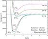Fig. 1 PECs of Λ – S states for the S2 molecule.

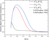Fig. 2 EDTMs between Λ – S states of S2.

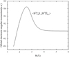Fig. 3 Orbital EAMC matrix elements between Λ – S states.

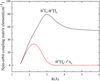Fig. 4 Absolute value of SOC matrix elements between Λ – S states.

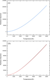Fig. 5 Temperature dependence of the partition functions of S2 computed using the $X^3{\mathrm{\Sigma }}_g^{-},B^{\mathrm{\prime }3}{\mathrm{\Pi }}_u,B^3{\mathrm{\Sigma }}_u^{-},b^1{\mathrm{\Sigma }}_g^{+},a^1{\mathrm{\Delta }}_g$, and f1Δu (a) and a1Δg and f1Δu (b) states.

3.2 Partition function and lifetime

According to Eq. (5), partition functions for S₂ calculated using the program ExoCross in steps of 15 up to 6000 K are provided in Fig. 5. Here, partition functions for S₂ are generated using the energy levels from refined model with the coupling effect method. There are six electronic states ($X^3{\mathrm{\Sigma }}_g^{-},B^{\mathrm{\prime }3}{\mathrm{\Pi }}_u,B^3{\mathrm{\Sigma }}_u^{-}$, $b^1{\mathrm{\Sigma }}_g^{+},a^1{\mathrm{\Delta }}_g$ and f¹Δ_u) involved in the calculation in Fig. 5a. To obtain the spectrum of the first excited a¹Δ_g state to the highly excited state f¹Δ_u, the partition function considers only two electronic states in Fig. 5b. For comparison, the calculated partition functions from Sauval & Tatum (1984) and Gomez et al. (2024) for different temperatures are listed in Table 3. The nuclear spin degeneracy, g_ns=1 for S₂, is used to provide the partition functions. When energy states are degenerate, the sum of partition functions needs to be multiplied by the degeneracy factor from Sauval & Tatum (1984) and Gomez et al. (2024). In the present work, the calculation of the partition function has considered all the energy levels of degenerate states. Thus, when comparing the partition from this study to values from the literature Sauval & Tatum (1984) and Gomez et al. (2024), it is necessary to multiply literature values by an integer value of 2 to obtain agreement. As shown in Table 3, the partition functions involving the six electronic states from this work agree well with the literature values below about 1200 K, and the agreement for the partition functions further decreases somewhat at higher temperatures due to the thermal occupation of higher energy electronic states.

Lifetimes were calculated using the refined model with the coupling effect by the LEVEL program. The calculated radiative lifetimes (τ) for the excited electronic states B′³Π_u and $B^3{\mathrm{\Sigma }}_u^{-}$ are presented Table 4 and compared to previous theoretical studies by Pradhan & Partridge (1996) and experimental measurements by Quick & Weston (1981). For the B′³Π_u state, our calculations show systematically shorter lifetimes (0.95–1.25 × 10⁻⁵ s) compared to Pradhan & Partridge (1996, 2.55–3.22 × 10⁻⁵ s) across all vibrational levels (v = 0–9). The absolute values differ by approximately a factor of 2.6; this consistent difference directly results from Pradhan’s omission of degeneracy in the transition probability calculations (Pradhan & Partridge 1996).

The $B^3{\mathrm{\Sigma }}_u^{-}$ state exhibits significantly shorter lifetimes (3.56–4.01 × 10⁻⁸ s), which is characteristic of stronger allowed transitions. Here, our results show excellent agreement with Pradhan & Partridge (1996) and Quick & Weston (1981), suggesting robust theoretical treatment for this state. The lifetimes of two excited states have been computed, providing important information regarding their respective roles in molecular dynamics and energy transfer processes.

3.3 Cross sections

The absorption cross sections for the transition f¹Δ_u ←a¹Δ_g at several temperatures (~300, 1000, 2000, and 3000 K) determined using the refined model are shown in Fig. 6a, with the largest cross- sections occurring at T=300 K and a wavenumber (v) of 41 190 cm⁻¹. This strongest UV spectrum exhibits cross sections of up to 1.04×10⁻¹⁶ cm²/molecule. Additionally, Fig. 6a displays similar peak cross sections at 1000, 2000, and 3000 K. Figure 6b illustrates the temperature dependence of the absorption cross sections for $B^3{\mathrm{\Sigma }}_u^{-},B^{\mathrm{\prime }3}{\mathrm{\Pi }}_u\leftarrow X^3{\mathrm{\Sigma }}_g^{-}$ using the refined model and considering the coupling effect. All spectra in this work have been calculated using Gaussian profiles with a half-width at half maximum (HWHM) of 0.1 cm⁻¹. In Fig. 6b, the infrared spectrum at 3000 K is significantly stronger than that at 300 K, while the peak cross section of the strongest UV spectrum (around 41 500 cm⁻¹) at 300 K is 1.22×10⁻¹⁶ cm²/molecule. As expected, the spectra become more pronounced and broader at higher temperatures.

The absorption cross sections for the triplet-triplet transitions $B^3{\mathrm{\Sigma }}_u^{-},B^{\mathrm{\prime }3}{\mathrm{\Pi }}_u\leftarrow X^3{\mathrm{\Sigma }}_g^{-}$ are illustrated in Fig. 7. Figure 7a compares the cross sections with data from Stark et al. (2018) and Gomez et al. (2024) at 370 K. At these lower wavenumbers, good agreement is observed with the spectra simulated using the line list from this work. Figure 7b shows an even better agreement: our spectra provide more extensive coverage and align closely with the Stark measurements (Stark et al. 2018). In summary, we validated the spectra generated in this work by comparing the calculated absorption cross sections to the measurements from Stark et al. (2018) and the estimates from Gomez et al. (2024) at 370 and 823 K.

3.4 Stick spectra

The spectrum intensity was generated by considering all lower and upper states with rotational levels J=0-120 and wavenumbers up to 70 000 cm⁻¹. These parameters are sufficient to model the experimental bands being considered. In 1970, 28 band systems of the f¹Δ_u ←a¹Δ_g transition of S₂ were photographed (Carleer & Colin 1970) using flash photolysis and flash discharge techniques at high resolution. Carleer & Colin (1970) analyzed these vibrational and rotational bands, providing a wide range of quantum numbers. In particular, they noted a few characteristic bands, including (4, 1), (10,0), and (11,0) of the f¹Δ_u ←a¹Δ_g vibronic transitions (see Fig. 8), although the intensities of the spectral lines were not provided. To understand these bands more intuitively, we simulated the absorption spectra of the f¹Δ_u ←a¹Δ_g transition system using a rotational temperature of ~300 K (see Fig. 8), including the (4, 1),(10, 0), and (11, 0) bands. The measured band heads for the vibrational transitions are observed at 37 747.38 cm⁻¹ for the (4,1) band, 40 825.98 cm⁻¹ for (10,0), and 41 202.234 cm⁻¹ for (11, 0) (Carleer & Colin 1970). Our theoretical calculations that use the refined energy method yield band head positions of 37 745, 40 820, and 41 196 cm⁻¹ for these respective transitions, which are in good agreement with experimental values. Although the intensity of the Q branch decreases rapidly with increasing J, it remains weak and difficult to detect. The (4, 1), (10, 0), and (11, 0) bands of the f¹Δ_u ←a¹Δ_g transition exhibit only the P and R branches arising from alternate components of the Λ-doubled levels. The intensities for these lines of the P and R branches increase first and then decrease with increasing wavenumber (Fig. 8).

Our predicted pure rotational spectrum for the $B^3{\mathrm{\Sigma }}_u^{-}\leftarrow X^3{\mathrm{\Sigma }}_g^{-}(5,0)$ absorption spectrum is shown in Fig. 9. A comparison between our spectrum simulated using the refined energy method and the experimental laser-induced fluorescence (LIF) spectrum reveals good consistency, with only a small difference in wavenumber. This slight discrepancy is attributed to the coupling effect of the states. The absorption spectra for the $B^{\mathrm{\prime }3}{\mathrm{\Pi }}_u\leftarrow X^3{\mathrm{\Sigma }}_q^{-}$ transition are designed to assist in identifying band features of S₂ at the rotational temperature. Typical LIF spectra for the (10, 0) and Ω=2 for (6, 3) bands of $B^{\mathrm{\prime }3}{\mathrm{\Pi }}_u\leftarrow X^3{\mathrm{\Sigma }}_g^{-}$ transition were produced by Green & Western (1996), with rotational assignments for these sub-bands determined (Green & Western 1996). It is regretful that these LIF spectra cover only a 20 cm⁻¹ region. As a result, we simulated the absorption spectra for (6, 3) and (10, 0) bands at 300 K over a larger range, as shown in Fig. 10. The strongest intensities for the (6, 3) and (10, 0) bands are on the order of 10⁻²³ and 10⁻¹⁸, respectively, indicating that the FCF between low vibrational levels of the ground states and the high vibrational levels of B′³Π_u is relatively large. The absorption spectra of both the P and R branches exhibit characteristically sharp peaks. However, the Q-branch transition is relatively weak, making it easily covered by the P and R branches. Therefore, sensitive detectors may be required for its detection.

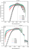Fig. 6 Absorption cross sections of f1Δu ←a1Δg (a) and $B^3{\mathrm{\Sigma }}_u^{-}$ and $B^{\mathrm{\prime }3}{\mathrm{\Pi }}_u\leftarrow X^3{\mathrm{\Sigma }}_g^{-}$ (b) for S2 simulated using the refined model with the coupling effect method. Temperatures of ~300, 1000, 2000, and 3000 K and Gaussian profiles HWHM=0.1 cm−1 are used.

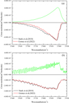Fig. 7 Experimental (below) and theoretical (above) absorption cross sections for two rovibronic S2 transitions, $B^3{\mathrm{\Sigma }}_u^{-}$ and $B^{\mathrm{\prime }3}{\mathrm{\Pi }}_u\leftarrow X^3{\mathrm{\Sigma }}_g^{-}$, at different temperatures: 370 (a) and 823 K (b). Gaussian profiles HWHM = 1 cm−1 are used.

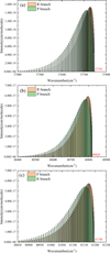Fig. 8 Simulated rotational P and R branches in the chosen vibronic band spectra for the f1Δu ←a1Δg transition: 4–1 band (a), 10-0 band (b), and 11-0 band (c). A rotational temperature of 300 K is used in the spectral modeling.

4 Conclusion

With the initial inspiration of wanting to understand S₂ in celestial environments, we conducted extensive calculations of spectra that include six electronic states ($X^3{\mathrm{\Sigma }}_g^{-},B^{\mathrm{\prime }3}{\mathrm{\Pi }}_u,B^3{\mathrm{\Sigma }}_u^{-}$, $b^1{\mathrm{\Sigma }}_g^{+},a^1{\mathrm{\Delta }}_g$, and f¹Δ_u) using the DUO program with the aim of facilitating a comprehensive spectral analysis. The calculations incorporate PECs, EDTMs, orbital EAMC, and SOC matrix elements, all determined using a high-level ab initio method and the refined energy method. This study predicts three transition systems (f¹Δ_u ←a¹Δ_g and $B^3{\mathrm{\Sigma }}_u^{-},B^{\mathrm{\prime }3}{\mathrm{\Pi }}_u\leftarrow X^3{\mathrm{\Sigma }}_g^{-}$) in the UV region. Partition functions were calculated and show good agreement with results from both Sauval & Tatum (two states) and Frances & Robert (three states) below approximately 1200 K.

The absorption spectra at different temperatures have been presented. Experimental and theoretical S₂ absorption cross sections for the $B^3{\mathrm{\Sigma }}_u^{-},B^{\mathrm{\prime }3}{\mathrm{\Pi }}_u\leftarrow X^3{\mathrm{\Sigma }}_g^{-}$ transitions at 370 and 823 K were compared. A good agreement is observed with the simulated cross section from this work. In addition, the absorption cross sections of the f¹Δ_u ←a¹Δ_g system for S₂ were simulated at temperatures of ~300, 1000, 2000, and 3000 K and with Gaussian profiles having a HWHM of 0.1 cm⁻¹. The experimental LIF spectrum of the $B^3{\mathrm{\Sigma }}_u^{-}\leftarrow X^3{\mathrm{\Sigma }}_g^{-}(5,0)$ band at a rotational temperature of approximately 300 K is well reproduced. Along the way, we expanded the regions of (6, 3) and (10, 0) bands for the $B^{\mathrm{\prime }3}{\mathrm{\Pi }}_u\leftarrow X^3{\mathrm{\Sigma }}_g^{-}$ system, critically identifying the intensities and regions of these bands for better comparison with astronomical spectral images. To facilitate the modeling of S₂ in astrophysical environments, an extensive spectrum that incorporates several important electronic states has been provided. Furthermore, the S₂ molecule possesses specific spectral characteristics that can be detected by astronomical observation tools, providing valuable information for studies of interstellar media and astrochemistry.

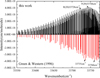Fig. 9 Experimental LIF spectrum (red) of the $B^3{\mathrm{\Sigma }}_u^{-}\leftarrow X^3{\mathrm{\Sigma }}_g^{-}(5,0)$ band of S2 with a rotational temperature of ~300 K, produced by the photolysis of H2S in a static cell from Green & Western (1996) compared to a spectrum (black) calculated using the refined model with the B′-B coupling effect method from this work.

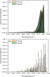Fig. 10 Spectra of these bands for the $B^{\mathrm{\prime }3}{\mathrm{\Pi }}_u\leftarrow X^3{\mathrm{\Sigma }}_g^{-}$ transition simulated using the refined model with the coupling effect method: 6-3 band (a) and 10-0 band (b). A rotational temperature of ~300 K is used in the spectral simulation.

Data availability

The data that support the findings of this study are available on Zenodo (Xiao, L.D 2025; The rovibronic spectra in UV absorption of S₂ [Data set].)

Acknowledgements

This work was supported by the National Natural Science Foundation of China (Grant No. 12274178, No. 11874177); the Ministry of Education and Science of Ukraine (Grant No. 0122U000760); the High Performance Computing Center (HPCC) of Jilin University and the high performance computing cluster Tiger@ IAMP.

References

All Tables

All Figures

	Fig. 1 PECs of Λ – S states for the S2 molecule.
In the text

	Fig. 2 EDTMs between Λ – S states of S2.
In the text

	Fig. 3 Orbital EAMC matrix elements between Λ – S states.
In the text

	Fig. 4 Absolute value of SOC matrix elements between Λ – S states.
In the text

	Fig. 5 Temperature dependence of the partition functions of S2 computed using the $X^3{\mathrm{\Sigma }}_g^{-},B^{\mathrm{\prime }3}{\mathrm{\Pi }}_u,B^3{\mathrm{\Sigma }}_u^{-},b^1{\mathrm{\Sigma }}_g^{+},a^1{\mathrm{\Delta }}_g$, and f1Δu (a) and a1Δg and f1Δu (b) states.
In the text

	Fig. 6 Absorption cross sections of f1Δu ←a1Δg (a) and $B^3{\mathrm{\Sigma }}_u^{-}$ and $B^{\mathrm{\prime }3}{\mathrm{\Pi }}_u\leftarrow X^3{\mathrm{\Sigma }}_g^{-}$ (b) for S2 simulated using the refined model with the coupling effect method. Temperatures of ~300, 1000, 2000, and 3000 K and Gaussian profiles HWHM=0.1 cm−1 are used.
In the text

	Fig. 7 Experimental (below) and theoretical (above) absorption cross sections for two rovibronic S2 transitions, $B^3{\mathrm{\Sigma }}_u^{-}$ and $B^{\mathrm{\prime }3}{\mathrm{\Pi }}_u\leftarrow X^3{\mathrm{\Sigma }}_g^{-}$, at different temperatures: 370 (a) and 823 K (b). Gaussian profiles HWHM = 1 cm−1 are used.
In the text

	Fig. 8 Simulated rotational P and R branches in the chosen vibronic band spectra for the f1Δu ←a1Δg transition: 4–1 band (a), 10-0 band (b), and 11-0 band (c). A rotational temperature of 300 K is used in the spectral modeling.
In the text

	Fig. 9 Experimental LIF spectrum (red) of the $B^3{\mathrm{\Sigma }}_u^{-}\leftarrow X^3{\mathrm{\Sigma }}_g^{-}(5,0)$ band of S2 with a rotational temperature of ~300 K, produced by the photolysis of H2S in a static cell from Green & Western (1996) compared to a spectrum (black) calculated using the refined model with the B′-B coupling effect method from this work.
In the text

	Fig. 10 Spectra of these bands for the $B^{\mathrm{\prime }3}{\mathrm{\Pi }}_u\leftarrow X^3{\mathrm{\Sigma }}_g^{-}$ transition simulated using the refined model with the coupling effect method: 6-3 band (a) and 10-0 band (b). A rotational temperature of ~300 K is used in the spectral simulation.
In the text

References

- A’Hearn, M. F., Feldman, P. D., & Schleicher, D. G. 1983, ApJ, 274, L99 [CrossRef] [Google Scholar]
- Anderson, W. R., Crosley, D. R., & Allen Jr, J. E. 1979, J. Chem. Phys., 71, 821 [Google Scholar]
- Barrow, R. F., & du Parcq, R. P. 1965, Elemental Sulfur, ed. B. Meyer (New York: Interscience) [Google Scholar]
- Barrow, R. F., & du Parcq, R. P. 1968, J. Phys. B: At. Mol. Phys., 1, 283 [Google Scholar]
- Bondybey, V. E., & English, J. H. 1978, J. Chem. Phys., 69, 1865 [Google Scholar]
- Bondybey, V. E., & English, J. H. 1979, J. Chem. Phys., 72, 3113 [Google Scholar]
- Carleer, M., & Colin, R. 1970, J. Phys. B: At. Mol. Phys., 3, 1715 [Google Scholar]
- da Silva, R. S., & Ballester, M. Y. 2019, Astrophys. Space Sci., 364, 169 [Google Scholar]
- De Almeida, A. A., & Singh, P. D. 1986, Earth Moon Planets, 36, 117 [Google Scholar]
- Donovan, R. J., Husain, D., & Jackson, P. T. 1968, Trans. Faraday Soc., 64, 1798 [Google Scholar]
- Feldman, P. D. 1984, Adv. Space Res., 4, 177 [Google Scholar]
- Francés-Monerris, A., Carmona-García, J., Trabelsi, T., et al. 2022, Nat. Commun., 13, 4425 [Google Scholar]
- Gomez, F., Hargreaves, R., & Gordon, I. E. 2024, MNRAS, 528, 3823 [Google Scholar]
- Green, M. E., & Western, C. M. 1996, J. Chem. Phys., 104, 848 [Google Scholar]
- Haranath, P. B. V. 1963, Zeitschrift für Physik, 173, 428 [Google Scholar]
- Herzberg, G. 1951, Van Nostrand Reinhold (New York, NY, USA) [Google Scholar]
- Hobbs, R., Rimmer, P. B., Shorttle, O., & Madhusudhan, N. 2021, MNRAS, 506, 3186 [NASA ADS] [CrossRef] [Google Scholar]
- Hrodmarsson, H. R., & Van Dishoeck, E. F. 2023, A&A, 675, A25 [NASA ADS] [CrossRef] [EDP Sciences] [Google Scholar]
- Ketteringham, J. M., & Barrow, R. F. 1964, Proc. Phys. Soc., 83, 330 [Google Scholar]
- Lewis, B. R., Gibson, S. T., Stark, G., & Heays, A. N. 2018, J. Chem. Phys., 148, 244303 [NASA ADS] [CrossRef] [Google Scholar]
- Maeder, R., & Miescher, E. 1948, Nature, 161, 393 [Google Scholar]
- Matsumi, Y., Suzuki, T., Munakata, T., & Kasuya, T. 1985, J. Chem. Phys., 83, 3798 [Google Scholar]
- McGrath, W. D., McGarvey, J. J., & Dempster, D. N. 1967, Can. J. Phys., 45, 2454 [Google Scholar]
- Minaev, B. F. 2000, Chem. Phys., 252, 25 [Google Scholar]
- Minaev, B. F., & Minaeva, V. A. 2001, Phys. Chem. Chem. Phys., 3, 720 [Google Scholar]
- Minaev, B. F., & Yashchuk, L. B. 2004, High. Energy. Chem., 38, 209 [Google Scholar]
- Minaev, B. F., Vahtras, O., & Ågren, H. 1996, Chem. Phys., 208, 299 [Google Scholar]
- Narasimham, N., & Gopol, K. 1965, Curr. Sci., 34, 454 [Google Scholar]
- Narasimham, N. A., & Bhagvat, K. M. N. 1965, Proc. Indian Acad. Sci. A, 61, 75 [Google Scholar]
- Narasimham, N. A., & Brody, J. K. 1964, Proc. Indian Acad. Sci. A, 59, 345 [Google Scholar]
- Naudé, S. M., & Christy, A. 1931, Phys. Rev., 37, 490 [Google Scholar]
- Noll, K. S., McGrath, M. A., Trafton, L. M., et al. 1995, Science, 267, 1307 [CrossRef] [Google Scholar]
- Patiño, P., & Barrow, R. F. 1982, J. Chem. Soc. Faraday Trans., 78, 1271 [Google Scholar]
- Pradhan, A. D., & Partridge, H. 1996, Chem. Phys. Lett., 255, 163 [NASA ADS] [CrossRef] [Google Scholar]
- Quick Jr, C. R., & Weston Jr, R. E. 1981, J. Chem. Phys., 74, 4951 [Google Scholar]
- Rosen, B., & Désirant, M. 1935, Bull. Soc. R. Sci. Liège, 6, 233 [Google Scholar]
- Sauval, A. J., & Tatum, J. B. 1984, ApJS, 56, 1937 [Google Scholar]
- Setzer, K. D., Kalb, M., & Fink, E. H. 2003, J. Mol. Spectrosc., 221, 127 [Google Scholar]
- Smith, W. H., & Liszt, H. S. 1971, J. Quant. Spectrosc. Radiat. Transfer, 11, 45 [Google Scholar]
- Spencer, J. R., Jessup, K. L., McGrath, M. A., Ballester, G. E., & Yelle, R. 2000, Science, 288, 1208 [Google Scholar]
- Stark, G., et al. 2018, J. Chem. Phys., 148, 244302 [NASA ADS] [CrossRef] [Google Scholar]
- Sun, Z. F., Farooq, Z., Parker, D. H., Martin, P. J. J., & Western, C. M. 2019, J. Phys. Chem. A, 123, 6886 [Google Scholar]
- Tanaka, Y., & Ogawa, M. 1962, J. Chem. Phys., 36, 726 [Google Scholar]
- Werner, H. J., Knowles, P. J., Knizia, G., Manby, F. R., & Schütz, M. 2012, WIREs Comput. Mol. Sci., 2, 242 [CrossRef] [Google Scholar]
- Wieland, K., Wehrli, M., & Miescher, E. 1934, Helv. Phys. Acta, 7, 841 [Google Scholar]
- Woon, D. E., & Dunning, T. H., Jr. 1993, J. Chem. Phys., 98, 1358 [NASA ADS] [CrossRef] [Google Scholar]
- Xiao, L. D., Yan, B., & Minaev, B. F. 2023, Phys. Chem., 3, 110 [Google Scholar]
- Xue, J. L., Yuan, X., Li, R., Liu, X. S., & Yan, B. 2020, Spectrochim. Acta A, 118679 [Google Scholar]
- Yurchenko, S. N., Lodi, L., Tennyson, J., & Stolyarov, A. V. 2016, Comput. Phys. Commun., 202, 262 [NASA ADS] [CrossRef] [Google Scholar]
- Yurchenko, S. N., Al-Refaie, A. F., & Tennyson, J. 2018, A&A, 614, A131 [NASA ADS] [CrossRef] [EDP Sciences] [Google Scholar]
- Zahnle, K., Mac Low, M. M., Lodders, K., & Fegley, B., Jr. 1995, Geophys. Res. Lett., 22, 1593 [Google Scholar]
All Tables
Comparison of de-perturbed vibrational energy levels (Tv,0; cm−1) for the and B′3Πu states with the experimental values (Green & Western 1996).
Comparison of de-perturbed vibrational energy levels (Tv,0; cm−1) for the state with the experimental (Green & Western 1996) and theoretical (Gomez et al. 2024) values.
Comparison of the calculated partition function, Q(T), with those of Sauval & Tatum (1984) and Gomez et al. (2024).