© The Authors 2025

1. Introduction

The origin and evolution of magnetic fields in radiative stellar interiors remain a fundamental challenge in astrophysics. Progress has been hindered by the absence of observational constraints for any class of stellar objects until recently, when high-precision asteroseismic measurements from the Kepler mission unveiled the internal magnetic fields of red giants (Li et al. 2022). The seismic detection relies on mixed modes – oscillation modes that act as gravity modes in the core and pressure modes in the envelope of these stars – which delivered first field strength estimates exceeding 100 kG due to the suppression of dipolar modes attributed to magnetic fields (Fuller et al. 2015). More recently, asymmetric splittings in the mixed modes’ frequency spectrum were measured in 13 low-mass evolved stars, indicating strong radial fields ranging from 20 to 150 kG (Li et al. 2022, 2023; Deheuvels et al. 2023). These asteroseismic measurements probe a narrow region of red giant cores and suggest that the radial field strength decreases from subgiants (SGs) to the red giant branch (RGB), i.e., with age. This breakthrough marks a new era in observational asteroseismology, spurring advances in inverse problems for stellar magnetism (e.g., Bhattacharya et al. 2024) and offering a unique opportunity to test and refine theoretical models of magnetic field generation and evolution in low-mass stars.

The high magnetic Reynolds number in radiative stellar interiors favors the buildup of strong toroidal magnetic fields. Differential rotation can efficiently wind up even weak poloidal fields into predominantly toroidal configurations. Purely toroidal fields in a radiative region are prone to various instabilities, including the shear-driven magnetorotational instability (Velikhov 1959; Balbus & Hawley 1991) or the magnetic buoyancy instability (Parker 1966; Gilman 1970). In strongly stably stratified fluids, it is generally accepted that the dominant instability is the one caused by electric currents that maintain the toroidal field configuration (Spruit 1999). Current-driven instabilities of pinches and torus configurations were initially studied for laboratory fusion research, neglecting the effect of gravity (e.g., Freidberg 1970; Goedbloed & Hagebeuk 1972). In the astrophysical context, Tayler (1973) was the first to consider, in cylindrical geometry, the adiabatic stability of purely toroidal fields in a stratified, nonrotating star. The author showed that regions near the poles are always unstable to nonaxisymmetric perturbations with the azimuthal wavenumber m = 1.

The nature of this kink-type instability, known as the Tayler instability, is significantly altered by the addition of an axial field, even when its strength is small compared to the toroidal component (Knobloch 1992). Although it reduces the growth rate, the presence of an axial field introduces a new resonant instability of the mixed toroidal-poloidal configuration at high vertical wavenumbers, a behavior confirmed by numerical simulations (Bonanno & Urpin 2008, 2011). The stability of mixed toroidal-poloidal field configurations in spherical symmetry was explored through direct numerical simulations (Braithwaite & Nordlund 2006; Duez et al. 2010), with the classic analytical solution by Prendergast (1956) often serving as a reference. However, recent work shows that this solution is prone to resistive instabilities, even under strongly stable stratification, raising questions about its suitability as a model for magnetic fields in stars (Kaufman et al. 2022).

Stratification and rotation have significant stabilizing effects on the Tayler instability of purely toroidal fields (Pitts & Tayler 1985; Spruit 1999; Skoutnev & Beloborodov 2024). Most linear perturbation analyses adopt a fully local approach based on the classical Wentzel–Kramers–Brillouin (WKB) approximation and use a cylindrical geometry valid near the poles of the star. In contrast, Bonanno & Urpin (2012) (hereafter BU12) performed a global analysis in radius, incorporating both stratification and thermal diffusion in a nonrotating sphere. Their results showed that, although gravity can significantly reduce the instability growth rate, σ, thermal diffusion prevents completesuppression. In the stellar regime of highly stable thermal stratification, in which the Brunt-Väisälä frequency, ω_BV, greatly exceeds the Alfvén frequency of the background axisymmetric toroidal field, ω_A, BU12 found that the growth rates of the least stable eigenmodes away from the poles – generally corresponding to the fundamental eigenmode not captured by fully local analyses – scale as

$$\begin{array}{c}\hfill \frac{\sigma }{{\omega }_{\mathrm{A}}}\sim {\left(\frac{{\omega }_{\mathrm{A}}}{{\omega }_{\mathrm{BV}}}\right)}^2.\end{array}$$(1)

A proper assessment of the dynamical impact of the Tayler instability in stellar interiors thus requires global analysis in a spherical geometry, as was demonstrated by BU12 and by Kitchatinov & Rüdiger (2008), whose study included disturbances that are global in latitude.

Although global linear analyses offer valuable insights, they rely on certain simplifying assumptions and cannot fully replace direct numerical simulations, which are essential to capture the full global character of the Tayler instability and its nonlinear behavior. However, numerical studies in spherical geometry – especially under strong stratification – remain limited. Early works by Arlt & Rüdiger (2011) and Szklarski & Arlt (2013) explored the instability in a spherical shell using the Boussinesq approximation, aiming to explain the observed surface magnetic fields of chemically peculiar intermediate-mass stars, but were restricted to moderately stratified cases. More recently, Guerrero et al. (2019) investigated the impact of stable stratification on the instability through simulations in a similar geometry, but within the anelastic approximation and neglecting viscous and resistive diffusion (for an analysis of the Tayler instability conditions under the anelastic approximation, see Goldstein et al. 2019). Their simulations confirmed a stabilizing influence of stratification, although they could not recover the scaling relation (1) predicted by BU12. Within the same framework, Monteiro et al. (2023) studied the combined effect of rotation and gravity. In the presence of differential rotation, Jouve et al. (2015, 2020) and Meduri et al. (2024) investigated numerically the interplay between the magnetorotational instability of predominantly toroidal fields and the Tayler instability.

In this work, we present direct numerical simulations of the Tayler instability of a purely toroidal field in a nearly full sphere, extending into the regime of strong stable stratification. For the first time, we systematically explore solutions ranging from subcritical to highly supercritical cases. Unlike the ones of Guerrero et al. (2019), our simulations incorporate both finite viscosity and magnetic diffusivity, and are initialized with a physically motivated background toroidal magnetic field whereby small deviations from the spherically symmetric equilibrium are attained by means of a nonspherically symmetric component of the pressure. Combining global linear perturbation theory and numerical simulations, we provide a unified picture of the Tayler instability in a sphere – capturing not only the small-scale modes known from WKB analyses, but also a new class of large-scale unstable fluctuations that emerge at low latitudes.

The remainder of the paper is organized as follows. In Sect. 2, we present a linear stability analysis of a purely toroidal field, global in radius, generalizing the one of BU12. We examine the properties of the unstable eigenmodes when varying the degree of stable stratification, first neglecting thermal diffusion and then including its effects. Section 3 presents 3D direct numerical simulations in the same spherical geometry and initialized with the same background toroidal field as the linear analysis. We investigate the stability of the relaxed axisymmetric solutions for different levels of stable stratification and compare the results with the predictions from the linear analysis. Our numerical simulation results yield two simple algebraic relations linking the threshold toroidal magnetic field strengths for instability onset and the transition between unstable regimes to key fluid properties. In Sect. 4, we combine these numerical results with stellar evolution models of low-mass stars to predict corresponding threshold fields in SG and red giant cores. Section 5 closes the paper with a summary of the results and key conclusions.

2. Linear perturbation analysis

2.1. Basic equations

Bonanno & Urpin (2012) considered the stability of a purely axisymmetric toroidal field, $\mathit{B}=B_{\varphi }(r,\theta ){\widehat{\mathit{e}}}_{\varphi }$, in a nonrotating stellar radiative region in spherical geometry. They neglected viscous and magnetic diffusion, but included thermal diffusion with thermal diffusivity, κ. In this work, (r, θ, ϕ) denote spherical coordinates with unit vectors $({\widehat{\mathit{e}}}_r,{\widehat{\mathit{e}}}_{\theta },{\widehat{\mathit{e}}}_{\varphi })$. The stability analysis is global in radius, but local in latitude and azimuth.

We extended the analysis of BU12 by including the latitudinal variations of the background toroidal field, which were previously neglected. In the latitudinal direction, our local approximation requires k_θ ≫ H_θ⁻¹, where k_θ = l/r, with l the latitudinal wavenumber, and H_θ = r∂lnB_ϕ/∂θ is the characteristic latitudinal scale of the background field. Stable thermal stratification was considered under the Boussinesq approximation. The fluid has uniform density, ρ, so gravity varies linearly with radius, $\mathit{g}=-g(r){\widehat{\mathit{e}}}_{\mathrm{r}}=-g_{\mathrm{out}}r/r_{\mathrm{out}}{\widehat{\mathit{e}}}_{\mathrm{r}}$. Here, g_out is the gravitational acceleration at the outer boundary of the radiative zone, located at radius r = r_out.

The background toroidal magnetic field varies linearly with the cylindrical radius, ϖ,

$$\begin{array}{c}\hfill B_{\varphi }\propto rsin\theta =\varpi .\end{array}$$(2)

With this field configuration, the local approximation above reads l ≫ cotθ and therefore the analysis cannot be applied too close to the symmetry axis. This basic state explicitly satisfies the magnetohydrostatic equilibrium

$$\begin{array}{c}\hfill -\frac{\mathbf{\nabla }P}{\rho }+\mathit{g}+\frac{1}{\mu \rho }(\mathbf{\nabla }\times \mathit{B})\times \mathit{B}=\mathbf{0},\end{array}$$(3)

which is the relevant force balance in a spherical stellar interior. Here, μ is the magnetic permeability of vacuum, and the total pressure is P = p(r)+h(r, θ), where p(r) is the hydrostatic spherically symmetric contribution balancing gravity, and h(r, θ)∝r²sin²θ is a non-spherically symmetric component whose gradient balances the Lorentz force. The field configuration (2) satisfies the classical instability criterion of Tayler (1973) for nonaxisymmetric perturbations with azimuthal wavenumber m = 1,

$$\begin{array}{c}\hfill \frac{\mathrm{d}ln{B}_{\varphi }}{\mathrm{d}ln\varpi }>-\frac{1}{2},\end{array}$$(4)

which is valid near the symmetry axis of a nonrotating star and in the absence of diffusivities. We note that WKB analyses typically assume a different background toroidal field configuration, B_ϕ ∝ sinθcosθ, which can arise from the shearing of a weak dipolar field by radial differential rotation (e.g., Spruit 1999; Fuller et al. 2019; Skoutnev & Beloborodov 2024).

We considered small amplitude perturbations to the background fluid velocity, u = 0, magnetic field, B, and temperature, T. We denote the perturbations to the fluid velocity, magnetic field, and temperature by u′, B′, and T′, respectively. Following BU12, we performed a normal mode analysis, seeking solutions of the form f′(r)exp(σt − ilθ − imϕ) to the linearized magnetohydrodynamic (MHD) equations. Here, t is time, σ = Re(σ) + i Im(σ), and f′(r) is a scalar function that stands for one of the components of the perturbed quantities. Linearizing the MHD equations around the basic state (3) and eliminating all variables in favor of the radial velocity perturbation, u_r′, and T′ as discussed in BU12, we obtained the two coupled ordinary differential equations

$$\begin{array}{cc}& [{\sigma }^2+{\omega }_{\mathrm{A}}^2-\frac{4{\omega }_{\mathrm{A}}^4{cos}^2\theta }{m^2({\sigma }^2+{\omega }_{\mathrm{A}}^2)}]\frac{{\mathrm{d}}^2{u}_r^{\prime }}{\mathrm{d}{r}^2}\hfill \\ \hfill & +\frac{4}{r}[{\sigma }^2+{\omega }_{\mathrm{A}}^2-\frac{4{\omega }_{\mathrm{A}}^4{cos}^2\theta }{m^2({\sigma }^2+{\omega }_{\mathrm{A}}^2)}-\mathrm{i}\frac{l{\omega }_{\mathrm{A}}^{4}sin2\theta }{m^2({\sigma }^2+{\omega }_{\mathrm{A}}^2)}]\frac{\mathrm{d}{u}_r^{\prime }}{\mathrm{d}r}\hfill \\ \hfill & +[\frac{2}{r^2}{\sigma }^2-k_{\perp }^2({\sigma }^2+{\omega }_{\mathrm{A}}^2)+\frac{4{\omega }_{\mathrm{A}}^2}{r^2}(\frac{k_{\perp }^2}{k_{\varphi }^2}-\frac{k_{\theta }^2}{k_{\varphi }^2}\frac{{\sigma }^2}{{\sigma }^2+{\omega }_{\mathrm{A}}^2}\hfill \\ \hfill & -\frac{2{\omega }_{\mathrm{A}}^2{cos}^2\theta }{m^2({\sigma }^2+{\omega }_{\mathrm{A}}^2)}-\mathrm{i}\frac{3l{\omega }_A^{2}sin\theta cos\theta }{m^2({\sigma }^2+{\omega }_{\mathrm{A}}^2)})]u_r^{\prime }=-k_{\perp }^2\alpha g\sigma T^{\prime },\hfill \end{array}$$(5)

$$\begin{array}{cc}& \frac{\kappa }{r^2}\frac{\mathrm{d}}{\mathrm{d}r}\left(r^2\frac{\mathrm{d}{T}^{\prime }}{\mathrm{d}r}\right)-(\sigma +\kappa k_{\perp }^2)T^{\prime }=\frac{{\omega }_{\mathrm{BV}}^2}{\alpha g_{\mathrm{out}}}{u}_r^{\prime }.\hfill \end{array}$$(6)

In the equations above, the Alfvén frequency of the background azimuthal field is

$$\begin{array}{c}\hfill {\omega }_{\mathrm{A}}=\frac{B_{\varphi }{k}_{\varphi }}{{(\mu \rho )}^{1/2}},\end{array}$$(7)

where k_ϕ = m/(rsinθ), and k_⊥² = k_θ² + k_ϕ². The Brunt-Väisälä frequency is defined by

$$\begin{array}{c}\hfill {\omega }_{\mathrm{BV}}^2=-g_{\mathrm{out}}\alpha ({\mathbf{\nabla }}_{\mathrm{ad}}T-\mathbf{\nabla }T)·{\widehat{\mathit{e}}}_r,\end{array}$$(8)

where α is the thermal expansion coefficient. The adiabatic temperature gradient is ${\widehat{\mathit{e}}}_r·{\mathbf{\nabla }}_{\mathrm{ad}}T={(\mathrm{d}T/\mathrm{d}r)}_{\mathrm{ad}}$ and the actual temperature gradient is subadiabatic, dT/dr >  (dT/dr)_ad. We employed the temperature gradient profile $({\mathbf{\nabla }}_{\mathrm{ad}}T-\mathbf{\nabla }T)·{\widehat{\mathit{e}}}_r=A(1/r_{\mathrm{out}}^2-1/r^2){(1/r_{\mathrm{out}}^2-1/r_{\mathrm{in}}^2)}^{-1}$, which decreases from A at the inner boundary, r_in, to 0 at the outer boundary, r_out. The perturbed magnetic field, B′, was obtained from the velocity perturbations through the linearized induction equation,

$$\begin{array}{c}\hfill \frac{\partial {\mathit{B}}^{\prime }}{\partial t}=\mathbf{\nabla }\times ({\mathit{u}}^{\prime }\times \mathit{B}).\end{array}$$(9)

As expected, in the limit of large radial wavenumbers, k_r ≫ k_θ ≫ H_θ⁻¹, our analysis is consistent with a purely local approach. Considering the radial part of the perturbations as f′ = exp(−i k_rr) and retaining only the leading-order terms in k_r in Eqs. (5) and (6), we obtain the dispersion relation

$$\begin{array}{c}\hfill ({\sigma }^2+{\omega }_{\mathrm{A}}^2+\frac{k_{\perp }^2}{k_r^2}{\omega }_{\mathrm{BV}}^2\frac{\sigma }{\sigma +\kappa k_r^2})({\sigma }^2+{\omega }_{\mathrm{A}}^2)-4\frac{{\omega }_{\mathrm{A}}^4}{m^2}{cos}^2\theta =0.\end{array}$$(10)

This dispersion relation matches the one obtained by the local analysis of Skoutnev & Beloborodov (2024) for our background toroidal field. As we show below, our linear analysis offers new insight into the influence of gravity on the Tayler instability in a sphere, overcoming key limitations of fully local approaches.

2.2. Numerical results

We nondimensionalized Eqs. (5) and (6) using the outer boundary radius, r_out, as the reference length scale. Time was scaled by the Alfvén frequency,

$$\begin{array}{c}\hfill {\omega }_{\mathrm{A}0}=\frac{B_0}{{(\mu \rho )}^{1/2}{r}_{\mathrm{out}}},\end{array}$$(11)

where B₀ is the background toroidal field strength at the equator on the outer boundary. Temperature perturbations were scaled by the amplitude of the background temperature gradient, A. The resulting dimensionless variables are: radius $\stackrel{\sim }{r}=r/r_{\mathrm{out}}$, radial velocity perturbation ${\stackrel{\sim }{u}}_r\prime =u_r\prime {\omega }_{\mathrm{A}0}^{-1}{r}_{\mathrm{out}}^{-1}$, and temperature perturbation $\stackrel{\sim }{T}\prime =T\prime A^{-1}{r}_{\mathrm{out}}^{-1}$. In this scaling scheme, Eqs. (5) and (6) read

$$\begin{array}{cc}& ({\mathrm{\Gamma }}^2+m^2-\frac{4m^2{cos}^2\theta }{{\mathrm{\Gamma }}^2+m^2})\frac{{\mathrm{d}}^2{\stackrel{\sim }{u}}_r^{\prime }}{\mathrm{d}{\stackrel{\sim }{r}}^2}\hfill \\ \hfill & +\frac{4}{\stackrel{\sim }{r}}({\mathrm{\Gamma }}^2+m^2-\frac{4m^2{cos}^2\theta }{{\mathrm{\Gamma }}^2+m^2}-\mathrm{i}\frac{l{m}^{2}sin2\theta }{{\mathrm{\Gamma }}^2+m^2})\frac{\mathrm{d}{\stackrel{\sim }{u}}_r^{\prime }}{\mathrm{d}\stackrel{\sim }{r}}\hfill \\ \hfill & +\{\frac{2{\mathrm{\Gamma }}^2}{{\stackrel{\sim }{r}}^2}-{\stackrel{\sim }{k}}_{\perp }^2({\mathrm{\Gamma }}^2+m^2)+\frac{4m^2}{{\stackrel{\sim }{r}}^2}[(\frac{l^2{sin}^2\theta }{m^2}+1)\hfill \\ \hfill & -\frac{l^2{sin}^2\theta }{m^2}\frac{{\mathrm{\Gamma }}^2}{{\mathrm{\Gamma }}^2+m^2}-\frac{2{cos}^2\theta }{{\mathrm{\Gamma }}^2+m^2}\hfill \\ \hfill & -\mathrm{i}\frac{3lsin\theta cos\theta }{{\mathrm{\Gamma }}^2+m^2}]\}{\stackrel{\sim }{u}}_r^{\prime }=-{\delta }^2{\stackrel{\sim }{k}}_{\perp }^2\mathrm{\Gamma }\stackrel{\sim }{r}{\stackrel{\sim }{T}}^{\prime },\hfill \end{array}$$(12)

$$\begin{array}{cc}& \frac{ϵ}{{\stackrel{\sim }{r}}^2}\frac{\mathrm{d}}{\mathrm{d}\stackrel{\sim }{r}}\left({\stackrel{\sim }{r}}^2\frac{\mathrm{d}{\stackrel{\sim }{T}}^{\prime }}{\mathrm{d}\stackrel{\sim }{r}}\right)-(\mathrm{\Gamma }+ϵ{\stackrel{\sim }{k}}_{\perp }^2){\stackrel{\sim }{T}}^{\prime }={\stackrel{\sim }{\omega }}_{\mathrm{BV}}^2{\stackrel{\sim }{u}}_r^{\prime }.\hfill \end{array}$$(13)

Here, ${\stackrel{\sim }{k}}_{\perp }^2=l^2/{\stackrel{\sim }{r}}^2+m^2/({\stackrel{\sim }{r}}^2{sin}^2\theta )$, Γ = σ/ω_A0, and the dimensionless Brunt-Väisälä frequency is ${\stackrel{\sim }{\omega }}_{\mathrm{BV}}={\omega }_{\mathrm{BV}}/{\omega }_{\mathrm{BV}0}$, where we defined ω_BV0² = αg_outA. In the equations above, there are two dimensionless parameters quantifying the relative importance of the three key timescales of the problem. The first is the stratification parameter,

$$\begin{array}{c}\hfill \delta =\frac{{\omega }_{\mathrm{BV}0}}{{\omega }_{\mathrm{A}0}},\end{array}$$(14)

and the second is the ratio of the thermal diffusion rate, ω_T = κ/r_out², to the Alfvén frequency,

$$\begin{array}{c}\hfill ϵ=\frac{{\omega }_T}{{\omega }_{\mathrm{A}0}}.\end{array}$$(15)

In radiative stellar interiors, the Brunt-Väisälä frequency is typically the highest of the three frequencies, reflecting strong stable stratification. The thermal diffusivity, κ, is usually much larger than both the kinematic viscosity and magnetic diffusivity, justifying our initial assumption of an inviscid and perfectly electrically conducting fluid. Provided that the toroidal magnetic field is not very weak, we therefore expect the following ordering of timescales:

$$\begin{array}{c}\hfill {\omega }_{\mathrm{BV}0}\gg {\omega }_{\mathrm{A}0}\gg {\omega }_T,\end{array}$$(16)

or, in terms of dimensionless parameters,

$$\begin{array}{c}\hfill ϵ\ll 1\ll \delta .\end{array}$$(17)

To avoid singularities at the center, we introduced a small inner core of radius ${\stackrel{\sim }{r}}_{\mathrm{in}}=r_{\mathrm{in}}/r_{\mathrm{out}}=0.1$. We employed impenetrable flow boundary conditions, ${\stackrel{\sim }{u}}_r\prime =0$ at both ${\stackrel{\sim }{r}}_{\mathrm{in}}=0.1$ and ${\stackrel{\sim }{r}}_{\mathrm{out}}=1$. The temperature perturbations, $\stackrel{\sim }{T}\prime$, were set to zero at both boundaries.

Hereafter we fixed the latitudinal wavenumber to l = 10 and ϵ to 10⁻². For this choice of l, the local approximation adopted in our analysis is not strictly valid near the poles, specifically for colatitudes θ ≲ 5°. However, we find no significant difference in the results when comparing θ = 5° with a higher value of 10°, where the local approximation is well satisfied. Equations (12) and (13), together with the boundary conditions above, define a nonlinear eigenvalue problem. We solved this system numerically using an eight-order centered finite-difference scheme for the radial derivatives. A radial grid of 4000 points was employed, which we verified to provide consistent numerical results across the full range of stable stratification levels considered.

Instability occurs when Re(Γ), the real part of Γ, is positive. For simplicity of notation, we define Re(Γ)=Γ and omit the superscript $\stackrel{\sim }{}$ for nondimensional quantities henceforth. Note that the coefficients of the linear equations depend on the colatitude θ, implying that the growth rate also varies with this quantity, i.e., Γ = Γ(θ). We confirmed that instability arises for the azimuthal wavenumber m = 1, while both the axisymmetric mode (m = 0) and higher-order modes (m >  1) remain stable, as expected for the adopted background field configuration. The next two sections examine the behavior of this m = 1 instability under increasing stable stratification, by varying δ from 0 to 10³. We first consider the case without thermal diffusion and then include its effects.

2.2.1. Diffusionless case

We begin by considering the case without thermal diffusion, ϵ = 0. We found two classes of unstable eigenmodes, the first operating at high latitudes and the second one in the equatorial region. The first class shares properties expected for the modes known from the WKB approximation, while the second one is completely distinct from the first, as we shall demonstrate below.

We now describe the first class of eigenmodes, focusing on a colatitude of θ = 5°. Figure 1a-c presents the radial profiles of the real part of the latitudinal field eigenmodes, Re(B_θ′), with a nearly adiabatic growth rate of Γ = 0.95, for different values of the stratification parameter δ. For all values of δ explored, the eigenmodes are largely confined in the inner half of the radial domain. This spatial structure is characteristic of all eigenmodes across the growth rate spectrum. The imaginary parts of the eigenmodes closely resemble the real ones and are therefore not shown here.

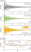Fig. 1. Radial profiles of the real parts of selected unstable latitudinal field eigenmodes, Re(Bθ′), in the absence of thermal diffusion (ϵ = 0). Panels (a)–(c) show the high-latitude eigenmodes (θ = 5°) with the nearly adiabatic growth rate of Γ = 0.95 for different values of the stratification parameter δ (see legend insets). The inset in (c) provides a zoom on the eigenmode between r = 0.10 and 0.12. Panel (d) displays the most unstable eigenmodes at the equator (θ = 90°); no unstable modes are found for δ ≥ 25. The horizontal axis is logarithmic in (a)–(c) and linear in (d).

Stable stratification impedes radial displacements and thereby determines the characteristic instability length scale in that direction. Classical local linear analyses show that, in the diffusionless limit, the radial wavenumber, k_r, of the m = 1 Tayler modes growing at the adiabatic rate, ω_A, satisfies (Spruit 1999; Skoutnev & Beloborodov 2024)

$$\begin{array}{c}\hfill k_r>k_{\theta }\frac{{\omega }_{\mathrm{BV}}}{{\omega }_{\mathrm{A}}}.\end{array}$$(18)

For the background state considered here, ω_BV/ω_A ∼ 1/r², implying that k_r decreases with increasing radius. This leads to a radial variation in the eigenmode scale, with longer wavelengths in the outer regions where stratification is weaker – consistent with the morphology observed in Fig. 1a-c.

Using the definitions of the previous section, Eq. (18) can be estimated as

$$\begin{array}{c}\hfill k_r{r}_{\mathrm{out}}>l\delta ,\end{array}$$(19)

where l = 10. We estimated the characteristic radial wavenumber of each eigenmode as k_r = π/λ_r, where λ_r = D/n is the mean half-wavelength. Here, n denotes the number of radial nodes (zero crossings) within the domain of extent D = r_out − r_in. Figure 2a presents k_r as a function of δ for the eigenmodes Re(B_θ′) with growth rates Γ = 0.8, 0.9, and 0.95. For all these high growth rates, which are close to the adiabatic value, the radial wavenumbers exceed the WKB limit given by Eq. (19) (dotted line) and converge toward the expected scaling for δ >  10. This confirms that our eigenvalue problem, in the limit of large k_r, recovers the WKB dispersion relation (10), thereby validating the numerical solver.

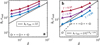Fig. 2. Radial wavenumber, kr, of various unstable eigenmodes, evaluated from the real part of Bθ′, as a function of δ for (a) no thermal diffusion (ϵ = 0) and (b) finite thermal diffusion (ϵ = 10−2). Triangles connected by solid lines indicate eigenmodes at colatitude θ = 5° with growth rates Γ = 0.8 (blue), 0.9 (purple), and 0.95 (red). Selected eigenmodes of the Γ = 0.95 tracks in (a) and (b) are displayed in Figs. 1a–c and 3a–c, respectively. The dotted lines denote the minimum unstable wavenumber predicted by the local linear theory (Eqs. (19) and (21)). Open gray circles connected by dashed lines correspond to the equatorial eigenmodes (Fig. 1d and dashed lines in Fig. 3d).

When moving away from the symmetry axis toward lower latitudes, the amplitude of the component of the buoyancy force in the cylindrical radial direction, ${\widehat{\mathit{e}}}_{\varpi }$ – which counteracts the destabilizing Lorentz force of the background field – progressively increases, thereby stabilizing the WKB-like eigenmodes discussed above. Such a geometrical effect on the stabilizing role of gravity in a sphere was already noted by Goossens & Tayler (1980) in their diffusionless stability analysis. For θ ≳ 70°, we find no unstable WKB-like eigenmode when δ ≥ 20. At the equator (θ = 90°), gravity completely opposes the unstable cylindrical radial motions, and we find no instability at all for δ ≥ 25. For δ <  25, stable stratification is weaker, and instability exists, but in the form of a new class of eigenmodes, as anticipated above. The most unstable magnetic field fluctuations are large-scale ones, exhibiting only one or a few radial nodes (Fig. 1d). As δ increases, the most unstable eigenmode shifts outward, toward regions where stable stratification is locally weaker. Unlike the WKB-like modes at high latitudes, which maintain growth rates near ω_A0 for all values of stratification explored, the most unstable equatorial eigenmodes show a sharp decline in growth rate, from Γ = 0.98 at δ = 0 to 0.19 at δ = 20.

2.2.2. Effect of thermal diffusivity

We now examine the influence of thermal diffusion on the instability, considering ϵ = 10⁻². Thermal diffusion weakens the effect of the stabilizing buoyancy force by damping the amplitude of the temperature perturbations in the buoyancy force on the right-hand side of Eq. (12), thereby modifying both the radial structure and growth rates of the unstable eigenmodes. As in the diffusionless case discussed above, we find two distinct classes of unstable eigenmodes: rapidly growing, WKB-like modes at high latitudes, and slower, large-scale eigenmodes near theequator.

In the presence of thermal diffusion, unstable WKB modes growing at the adiabatic rate, ω_A, have radial wavenumbers that satisfy the condition (Spruit 1999; Skoutnev & Beloborodov 2024)

$$\begin{array}{c}\hfill k_r^4>k_{\theta }^2\frac{{\omega }_{\mathrm{BV}}^2}{{\omega }_{\mathrm{A}}\kappa }.\end{array}$$(20)

Using the definitions introduced earlier, this condition can be recast in nondimensional form as

$$\begin{array}{c}\hfill k_r{r}_{\mathrm{out}}>{(l\delta )}^{1/2}{ϵ}^{-1/4}.\end{array}$$(21)

We first demonstrate that, at high latitudes, the less stable eigenmodes from our linear analysis share salient characteristics with such pure WKB modes. As in the diffusionless case, eigenmodes at colatitude θ = 5° and for δ ≤ 50 display large growth rates and remain confined to the inner half of the radial domain. This is illustrated in Fig. 3a,b, which shows the radial profiles of Re(B_θ′) with nearly adiabatic growth rates, Γ = 0.95. Due to the effect of thermal diffusion, the radial length scales of these eigenmodes are larger than those of the corresponding diffusionless case, for all values of δ explored – as expected (cf. Fig. 3b and Fig. 1c for the case at δ = 50). The radial variation in the length scales of the eigenmodes, arising from the background stratification profile, appears less pronounced than in the absence of diffusion. For δ >  50, the dominant eigenmodes exhibit a different morphology, with significant amplitudes extending into the outer regions of the radial domain (Fig. 3c for δ = 500). The radial wavenumber, k_r, estimated from Re(B_θ′) as was discussed in the previous section, falls above the predicted WKB limit (Eq. (21); dotted line in Fig. 2b) for the eigenmodes with nearly adiabatic growth rates Γ = 0.95, as expected (Fig. 2b, red triangles). The WKB scaling, k_rr_out ∝ δ^1/2, is closely approached for δ >  200.

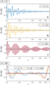Fig. 3. Same as Fig. 1 but for ϵ = 10−2. In panel (d), dashed and solid lines correspond to the type I and type II equatorial eigenmodes, respectively (see text for details). Type I eigenmodes are the most unstable (see Fig. 4 for their growth rate values). The horizontal axis is logarithmic in all panels.

Due to the geometrical reasons discussed above, the stabilizing effect of stratification on the unstable motions increases with colatitude and peaks at the equator. As in the diffusionless case, no WKB-like eigenmodes are found at colatitudes of θ ≳ 70°. However, the instability persists in the form of a distinct class of eigenmodes characterized by large radial length scales and significantly reduced growth rates. At the equator (θ = 90°), these global eigenmodes exhibit two distinct types of morphologies. The first, which we refer to as type I, corresponds to the most unstable modes and is characterized by confinement near the inner boundary (Fig. 3d, dashed lines). The radial wavenumber k_r of these eigenmodes initially increases with δ, but saturates for δ ≥ 10² (Fig. 2b, circles; Fig. 3d, dashed lines). Their growth rate strongly decreases with stratification, from Γ = 0.98 for δ = 5 to a value as small as 0.012 in the highly stratified case at δ = 500.

The second type of equatorial eigenmodes, referred to as type II hereafter, have lower growth rates than type I modes (for example, Γ = 0.41 and 6 × 10⁻³ for δ = 50 and 500, respectively). Similar to the eigenmodes reported by BU12, type II eigenmodes are distributed primarily in the outer half of the radial domain at higher levels of stable stratification (Fig. 3d, solid lines).

Figure 4 presents the growth rate of the type I equatorial eigenmodes, Γ_max, as a function of δ. For weak up to moderate stratification values of δ = 200, the growth rate slowly decreases as stratification increases, but always remaining on the order of the background Alfvén frequency, ω_A0. In the highly stratified regime in which δ >  200, the growth rate decreases more steeply, following the scaling

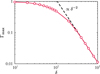Fig. 4. Dimensionless growth rates of the type I equatorial eigenmodes, Γmax, as a function of the stratification parameter δ for ϵ = 10−2. The dashed line indicates the scaling predicted by Bonanno & Urpin (2012), Γmax ∝ δ−2.

$$\begin{array}{c}\hfill {\mathrm{\Gamma }}_{\max }\propto {\delta }^{-2}\end{array}$$(22)

already predicted by BU12 (dashed line). The growth rates of the type II equatorial eigenmodes show the same scaling with δ and are therefore not presented here.

Unlike fully local approaches, our linear analysis successfully captures the global radial structure of the instability and allowed us to identify a new class of large-scale unstable modes developing at low latitudes. To extend the analysis beyond the local approximation in latitude and to include viscous and resistive effects, we now turn to self-consistent direct numerical simulations, which we present in the next section.

3. Direct numerical simulations

3.1. Governing equations

As in the linear analysis above, we considered a MHD fluid confined to a wide-gap spherical shell of aspect ratio χ = r_in/r_out = 0.1, where r_in and r_out denote the inner and outer boundary radii, respectively. The fluid has uniform density, ρ, gravity varies linearly with radius, $\mathit{g}=-g(r){\widehat{\mathit{e}}}_r=-g_{\mathrm{out}}r/r_{\mathrm{out}}{\widehat{\mathit{e}}}_r$, and stable thermal stratification was considered under the Boussinesq approximation as in the linear analysis. Here, g_out is the gravitational acceleration at the outer boundary. Unlike the linear analysis, we considered a viscous fluid with finite electrical conductivity. The kinematic viscosity, magnetic diffusivity, and thermal diffusivity of the fluid are ν, η, and κ, respectively.

We employed the mid-shell radius, r₀ = r_in + D/2, where D = r_out − r_in denotes the spherical shell gap, as the reference length scale, and the magnetic diffusion time, r₀²/η, as the reference timescale. Hereafter, all nondimensional variables are denoted by a tilde, unless explicitly defined otherwise. The magnetic field B is scaled in units of (μρ)^1/2η/r₀, where μ is the magnetic permeability of vacuum. Note that the dimensionless magnetic field strength, $|\stackrel{\sim }{\mathit{B}}|$, coincides with the Lundquist number

$$\begin{array}{c}\hfill \mathrm{Lu}=\frac{|\mathit{B}|r_0}{{(\mu \rho )}^{1/2}\eta }.\end{array}$$(23)

The fluid velocity is expressed in units of η/r₀. The non-hydrostatic pressure, Π, is scaled with ρη²/r₀². The scale for the temperature is ΔT = T_out − T_in >  0, the imposed background temperature contrast between the isothermal outer and inner boundaries that establishes stable stratification.

In this scaling scheme, the dimensionless equations governing the evolution of the fluid velocity, $\stackrel{\sim }{\mathit{u}}$, the magnetic field, $\stackrel{\sim }{\mathit{B}}$, and the temperature perturbations, $\stackrel{\sim }{\vartheta }$, around the background temperature, ${\stackrel{\sim }{T}}_{\mathrm{c}}$, are:

$$\begin{array}{c}\hfill \begin{array}{cc}\hfill \frac{\partial \stackrel{\sim }{\mathit{u}}}{\partial \stackrel{\sim }{t}}+(\stackrel{\sim }{\mathit{u}}·\stackrel{\sim }{\mathbf{\nabla }})\stackrel{\sim }{\mathit{u}}=& -\stackrel{\sim }{\mathbf{\nabla }}\stackrel{\sim }{\mathrm{\Pi }}+{\delta }_0^2{\mathrm{Lu}}_0^2\frac{r}{r_{\mathrm{out}}}\stackrel{\sim }{\vartheta }{\widehat{\mathit{e}}}_{\mathrm{r}}+\mathrm{Pm}{\stackrel{\sim }{\mathbf{\nabla }}}^2\stackrel{\sim }{\mathit{u}}\hfill \\ \hfill & +(\stackrel{\sim }{\mathbf{\nabla }}\times \stackrel{\mathbf{\sim }}{\mathit{B}})\times \stackrel{\sim }{\mathit{B}},\hfill \end{array}\end{array}$$(24)

$$\begin{array}{c}\hfill \frac{\partial \stackrel{\sim }{\mathit{B}}}{\partial \stackrel{\sim }{t}}=\stackrel{\sim }{\mathbf{\nabla }}\times (\stackrel{\sim }{\mathit{u}}\times \stackrel{\sim }{\mathit{B}})+{\stackrel{\sim }{\mathbf{\nabla }}}^2\stackrel{\sim }{\mathit{B}},\end{array}$$(25)

$$\begin{array}{c}\hfill \frac{\partial \stackrel{\sim }{\vartheta }}{\partial \stackrel{\sim }{t}}+(\stackrel{\sim }{\mathit{u}}·\stackrel{\sim }{\mathbf{\nabla }})\stackrel{\sim }{\vartheta }+(\stackrel{\sim }{\mathit{u}}·\stackrel{\sim }{\mathbf{\nabla }}){\stackrel{\sim }{T}}_{\mathrm{c}}=\frac{\mathrm{Pm}}{\mathrm{Pr}}{\stackrel{\sim }{\mathbf{\nabla }}}^2\stackrel{\sim }{\vartheta }.\end{array}$$(26)

The flow and the magnetic field obey solenoidality,

$$\begin{array}{c}\hfill \stackrel{\sim }{\mathbf{\nabla }}·\stackrel{\sim }{\mathit{u}}=0\mathrm{and}\stackrel{\sim }{\mathbf{\nabla }}·\stackrel{\sim }{\mathit{B}}=0.\end{array}$$(27)

The background temperature, ${\stackrel{\sim }{T}}_{\mathrm{c}}=T_{\mathrm{c}}/\mathrm{\Delta }T$, is the solution to the heat conduction equation ${\stackrel{\sim }{\mathbf{\nabla }}}^2{\stackrel{\sim }{T}}_{\mathrm{c}}=0$,

$$\begin{array}{c}\hfill {\stackrel{\sim }{T}}_{\mathrm{c}}=-c_1/\stackrel{\sim }{r}+c_2,\end{array}$$(28)

where $\stackrel{\sim }{r}=r/r_0$, and the coefficients c₁ = 2χ/(1 − χ²) and c₂ = 1 + (1 − χ)⁻¹ are determined by the imposed inner and outer boundary values of ${\stackrel{\sim }{T}}_{\mathrm{in}}=1$ and ${\stackrel{\sim }{T}}_{\mathrm{out}}=2$, respectively. The Brunt-Väisälä frequency, N, is related to this temperature profile by

$$\begin{array}{c}\hfill N^2(r)=g\alpha \frac{\mathrm{d}{T}_{\mathrm{c}}}{\mathrm{d}r},\end{array}$$(29)

where α is the coefficient of thermal expansion. We define a reference value for the Brunt-Väisälä frequency, N₀, as

$$\begin{array}{c}\hfill N_0^2=g_{\mathrm{out}}\alpha \frac{\mathrm{\Delta }T}{r_0}.\end{array}$$(30)

In Eqs. (24)–(26), there are four dimensionless control parameters. The first is the stratification parameter

$$\begin{array}{c}\hfill {\delta }_0=\frac{N_0}{{\omega }_{\mathrm{A}0}},\end{array}$$(31)

where ω_A0 = B₀r₀⁻¹(μρ)^−1/2 is the Alfvén frequency based on the initial magnetic field strength, B₀, which is defined below. Note that this definition of ω_A0 differs from Eq. (11), which is used throughout Sect. 2. The second parameter is the initial Lundquist number,

$$\begin{array}{c}\hfill {\mathrm{Lu}}_0=\frac{B_0{r}_0}{{(\mu \rho )}^{1/2}\eta }.\end{array}$$(32)

The remaining two parameters are the Prandtl number, Pr = ν/κ, and the magnetic Prandtl number, Pm = ν/η. At both spherical boundaries, we imposed impenetrable, stress-free boundary conditions for the flow, and perfect conductor conditions for the magnetic field.

To solve the problem above, we employed the open-source pseudo-spectral MHD code MagIC¹ (Wicht 2002; Schaeffer 2013). The numerical method is described in detail in Christensen & Wicht (2007) and we therefore mention only the essentials here. The code uses a poloidal-toroidal decomposition of the vector fields $\stackrel{\sim }{\mathit{u}}$ and $\stackrel{\sim }{\mathit{B}}$. The associated poloidal and toroidal potentials, along with the temperature, were expanded using spherical harmonic functions in the latitudinal and azimuthal directions. In the radial direction, a Chebyshev collocation method with N_r grid points was employed. The discretized equations were evolved in time using an implicit-explicit scheme, with the nonlinear terms handled explicitly. The numerical spatial resolutions were set to adequately capture the characteristic radial and angular length scales of the instability during both its linear growth and nonlinear evolution (see Sect. 3.4). For the highest degrees of stratification explored, we employed a maximum resolution of N_r = 321 radial grid points and ℓ_max = m_max = 213, where ℓ_max and m_max denote the maximum spherical harmonic degree and order, respectively.

3.2. Initial magnetic field configuration and values of the dimensionless parameters

As the initial condition for the magnetic field, we considered a purely axisymmetric azimuthal field of the form

$$\begin{array}{c}\hfill \stackrel{\sim }{\mathit{B}}(\stackrel{\sim }{t}=0)={\mathrm{Lu}}_0\stackrel{\sim }{r}sin\theta {\widehat{\mathit{e}}}_{\varphi }.\end{array}$$(33)

Before studying the stability of such a field configuration, we first investigated its temporal evolution when varying the strength of the stable stratification and the field amplitude. The stratification parameter, δ₀, spans values from 0 (corresponding to an unstratified flow) up to 900, while the Lundquist number, Lu₀, ranges from subcritical values, for which no instability is observed, to approximately 7300. The magnetic Prandtl number Pm was fixed to 1. When varying Lu₀ at fixed δ₀, to maintain a constant ratio of the thermal diffusion rate to the Alfvén frequency at ϵ₀ = ω_T/ω_A0 = 0.11, we adjusted the Prandtl number Pr accordingly. Here, the thermal diffusion rate is defined as ω_T = κ/r₀², and ϵ₀ can be expressed in terms of the basic input parameters as ϵ₀ = Pm Pr⁻¹ Lu₀⁻¹. Table 1 lists the input parameters of all simulation runs.

In contrast to the outer regions of red giant cores, the Prandtl number and the magnetic Prandtl number attain relatively high values in the inner, electron degenerate layers – values that are accessible to numerical simulations. Stellar evolution models indicate typical values of Pr ∼ 10⁻³ (Garaud et al. 2015) and 10⁻¹ ≲ Pm ≲ 10 (Rüdiger et al. 2015) for the degenerate cores of RGB stars with masses near that of the Sun. The value Pm = 1 adopted in this study lies within this range, while the employed values of Pr are, in most cases, only one order of magnitude larger (see Table 1).

Hereafter, we denote the azimuthal and meridional averages of an arbitrary function f(r, θ, ϕ, t) with angular brackets and an overbar, respectively,

$$\begin{array}{cc}\hfill ⟨f⟩& =\frac{1}{2\pi }{\displaystyle {\int }_0^{2\pi }}f\mathrm{d}\varphi \mathrm{and}\hfill \end{array}$$(34)

$$\begin{array}{cc}\hfill \overline{f}& =\frac{1}{\mathrm{A}}{\displaystyle {\int }_0^{\pi }{\int }_{r_{\mathrm{in}}}^{r_{\mathrm{out}}}}fr\mathrm{d}r\mathrm{d}\theta ,\hfill \end{array}$$(35)

where A is the area of half the meridional plane. The nonaxisymmetric fluid velocity and magnetic field are denoted by a prime. For example, the nonaxisymmetric azimuthal magnetic field is given by $\stackrel{\sim }{B}{\prime }_{\varphi }={\stackrel{\sim }{B}}_{\varphi }-⟨{\stackrel{\sim }{B}}_{\varphi }⟩$.

3.3. Background axisymmetric configuration

We first explored the slow, long-term evolution of the axisymmetric toroidal field due to resistive effects, by focusing on a Lundquist number of Lu₀ = 917 and varying the strength of stable stratification.

The temporal evolution of the volume integrated toroidal magnetic energy, $E_{\mathrm{mag}}^{\mathrm{tor}}=\frac{1}{2}{\displaystyle \int {\stackrel{\sim }{B}}_{\mathrm{tor}}^2}\mathrm{d}\stackrel{\sim }{V}$, is presented by the black lines in Fig. 5 for the unstratified case (δ₀ = 0), an intermediately stable stratification (δ₀ = 300), and a highly stable stratification (δ₀ = 900). The magnetic field remains axisymmetric throughout its evolution and is purely toroidal, as no poloidal component is initialized in our simulations. For all values of δ₀, the toroidal field decays exponentially due to Ohmic diffusion as expected. The snapshots in Fig. 6 demonstrate that the axisymmetric azimuthal field, $⟨{\stackrel{\sim }{B}}_{\varphi }⟩$, preserves the cylindrical symmetry of its initial state. Its configuration is modified exclusively toward the spherical boundaries to conform to the perfect conductor boundary conditions.

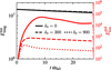Fig. 5. Temporal evolution of the volume integrated toroidal magnetic energy (black lines) and poloidal kinetic energy (red lines). Results are shown for the unstratified run (δ0 = 0) and two stratified runs (δ0 = 300 and 900). The Lundquist number is Lu0 = 917. Both the flow and magnetic field remain purely axisymmetric throughout the evolution.

We observe an initial rapid growth of the poloidal kinetic energy, $E_{\mathrm{kin}}^{\mathrm{pol}}=\frac{1}{2}{\displaystyle \int {\stackrel{\sim }{u}}_{\mathrm{pol}}^2}\mathrm{d}\stackrel{\sim }{V}$ (red lines in Fig. 5), driven by the development of meridional flows induced by the Lorentz force. These flows subsequently relax to their end-state configuration within some Alfvén travel times. The amplitude of these flows decreases with increasing δ₀, consistent with the restoring buoyancy force inhibiting radial motions. In the unstratified run, the meridional flow exhibits a single large-scale circulation cell in each hemisphere (black isocontour lines in Fig. 6a). With increasing stable stratification, the meridional flow becomes confined near the outer boundary, forming thin circulation cells that locally advect the azimuthal field (Fig. 6b,c). Over longer timescales, the meridional flow amplitude decays, mirroring the behavior of the toroidal field and confirming their magneticorigin.

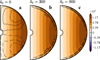Fig. 6. Snapshots of the three axisymmetric simulation runs presented in Fig. 5. Snapshot times tωA0 are 26.6 for (a) δ0 = 0, 26.9 for (b) δ0 = 300, and 27.3 for (c) δ0 = 900. Color contours show the axisymmetric azimuthal field, $⟨{\stackrel{\sim }{B}}_{\varphi }⟩$. Black contour lines represent the meridional circulation, with solid and dashed lines indicating clockwise and counterclockwise flows, respectively.

3.4. Stability to nonaxisymmetric perturbations

We investigated the stability of the background axisymmetric configurations in response to weak nonaxisymmetric perturbations. The perturbations are introduced at times t = t₁ (indicated in Table 1) and consist of spatially uncorrelated white noise in the nonaxisymmetric (m >  0) component of the toroidal magnetic field potential. The root mean square (RMS) amplitude of these perturbations is at least four orders of magnitude lower than that of the background axisymmetric azimuthal field.

As was demonstrated in the previous section, the axisymmetric azimuthal field strength decreases over time, and the field morphology shows mild variations with δ₀. To account for these changes, we defined a local version of the stratification parameter at the perturbation time,

$$\begin{array}{c}\hfill {\delta }_1=\frac{N}{{\omega }_{\mathrm{A}1}},\end{array}$$(36)

where ω_A1 = B_ϕ1r₀⁻¹(μρ)^−1/2 is the Alfvén frequency of the axisymmetric azimuthal field at the perturbation time B_ϕ1(r, θ)=⟨B_ϕ(r, θ, ϕ, t₁)⟩. The parameter δ₁ exhibits approximate cylindrical symmetry, with some modulations introduced by the chosen Brunt-Väisälä frequency profile, and varies roughly as $1/({\stackrel{\sim }{r}}^{2}sin\theta )$ within the fluid domain. To characterize the degree of stable stratification at the perturbation time, we define a mean value of the stratification parameter as ${\overline{\delta }}_1=\overline{N}/{\overline{\omega }}_{\mathrm{A}1}$, which is reported in Table 1 for all runs. Similarly, the characteristic azimuthal field strength at the perturbation time is represented by the mean Lundquist number, ${\overline{\mathrm{Lu}}}_1={\overline{B}}_{\varphi 1}{r}_0{\eta }^{-1}{(\mu \rho )}^{-1/2}$. This parameter can be interpreted as the ratio of the mean Alfvén frequency, ${\overline{\omega }}_{\mathrm{A}1}$, to the magnetic diffusion rate, ω_η = η/r₀².

We analyzed the stability of a set of axisymmetric simulation runs in which stable stratification increases up to ${\overline{\delta }}_1=321$, while the dimensionless field strength spans from ${\overline{\mathrm{Lu}}}_1=3$ to 5481. The ratio of the thermal diffusion rate to the mean Alfvén frequency at the perturbation time is ${\overline{ϵ}}_1={\omega }_T/{\overline{\omega }}_{\mathrm{A}1}$. This parameter is related to the other dimensionless quantities by ${\overline{ϵ}}_1=\mathrm{Pm}/(\mathrm{Pr}{\overline{\mathrm{Lu}}}_1)$ and its value is of 0.15 in all runs explored. In the following section, we focus on a representative case without stratification, where the Tayler instability exhibits its known WKB-like behavior. The influence of stable stratification and the various instability regimes identified are presented in Sect. 3.4.2.

3.4.1. Tayler instability without stratification

We begin by examining the stability of the unstratified run described in Sect. 3.3. The nonaxisymmetric perturbations are introduced at time $t_1=26.6{\omega }_{\mathrm{A}0}^{-1}$ when ${\overline{\mathrm{Lu}}}_1=677$ (see Fig. 6a for the background field configuration). This value of ${\overline{\mathrm{Lu}}}_1$ exceeds the threshold for instability onset by more than a factor of 20 (see Table 1). This simulation is hereafter designated as run TU0 and establishes a reference case for the characterization of the m = 1 Tayler instability.

Figure 7 shows the temporal evolution of the toroidal and poloidal magnetic energies for the azimuthal modes m = 0 to m = 6 in this run. Approximately $2/{\overline{\omega }}_{\mathrm{A}1}$ after the perturbation time, the first mode to grow exponentially is m = 1, as expected for the Tayler instability. The linear growth rate of the RMS toroidal field associated with this mode is ${\sigma }_{m=1}=1.1{\overline{\omega }}_{\mathrm{A}1}$, when evaluated in the period $(t-t_1){\overline{\omega }}_{\mathrm{A}1}=6.5-10.5$ (dashed black line in Fig. 7a). This value closely matches the rate calculated from the evolution of the m = 1 poloidal field (solid orange line in Fig. 7b). The background axisymmetric (m = 0) azimuthal field decays slowly due to Ohmic diffusion, with its evolution appearing nearly stationary during the linear growth phase of the instability (solid black line in Fig. 7a).

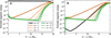Fig. 7. Temporal evolution of the (a) toroidal and (b) poloidal magnetic energies for the azimuthal modes m = 0 to m = 6 in the unstratified run TU0. The dashed black lines show exponential fits to the energy evolution of the m = 1 mode within the time interval $6.5\le (t-t_1){\overline{\omega }}_{\mathrm{A}1}\le 10.5$. These fits are used to determine the instability growth rates σ discussed in the text.

As was expected, snapshots of the nonaxisymmetric latitudinal field, ${\stackrel{\sim }{B}}_{\theta }\prime$, during the linear phase of the instability growth reveal a distinct m = 1 azimuthal symmetry (Fig. 8a,b). All the other nonaxisymmetric field and flow components exhibit the same symmetry and are therefore not shown here. There is no azimuthal drift of the nonaxisymmetric flow and field components, as expected in the absence of rotation (e.g., Rüdiger et al. 2012). The instability remains stationary also in the vertical direction and predominantly localizes in a wedge-shaped region around the vertical symmetry axis (Fig. 8d,f). This latter characteristic aligns with predictions from our linear analysis, which indicates that the growth rates of the unstable eigenmodes decrease with the colatitude θ, and is also consistent with previous results obtained from local linear stability studies in spherical geometry (Goossens & Tayler 1980). Our linear analysis also indicates that the characteristic radial wavenumber of the instability increases from the equator toward higher latitudes (black lines in Fig. 1a,d), which qualitatively matches the structure of the instability in run TU0. We refrain from making a direct quantitative comparison between the numerical simulation results and the linear analysis due to the limitations inherent in the latter’s approximations. In particular, the linear analysis may become questionable at higher latitudes near the symmetry axis, where the local approximation in the latitudinal direction is only partially satisfied. Additionally, the linear analysis neglects viscous and resistive effects, which would certainly influence the spectrum of the unstable radial modes if they were included. Finally, we note that the structure of the instability in run TU0 closely resembles that observed in global numerical studies of the Tayler instability in cylindrical geometry (Rüdiger et al. 2012; Ji et al. 2023).

Figure 7 shows that modes m >  1, as well as the axisymmetric poloidal field (black line in the right panel), are subcritical initially. They begin to grow only at times $t-t_1\gtrsim 10/{\overline{\omega }}_{\mathrm{A}1}$, as a result of nonlinear energy transfer from the large-amplitude m = 1 mode. A simple weakly nonlinear analysis of the ideal induction equation by Ji et al. (2023) predicts that the nonlinear growth rates of the m = 0 and m = 2 modes are 2 σ_m = 1. Higher chains of nonlinear interaction provide a nonlinear growth rate of m σ_m = 1 for modes m >  2. Figure 7b demonstrates that the nonlinear growth of the m = 0 and m = 2 poloidal field occurs at the same rate of $2.2{\overline{\omega }}_{\mathrm{A}1}$, which is twice the rate of the m = 1 mode, as anticipated. The nonlinear growth rates of the higher order modes in Fig. 7 are also in good agreement with the weakly nonlinear theory predictions. For simplicity, we hereafter denote the growth rate of the m = 1 mode as σ.

The instability shows an apparent saturation at $t-t_1\approx 18/{\overline{\omega }}_{\mathrm{A}1}$ when the nonaxisymmetric toroidal energy reaches values comparable to those of the background azimuthal field (Fig. 7a), with the nonaxisymmetric poloidal and toroidal energies roughly in equipartition. The field solution looses its simple azimuthal symmetry and transitions into a turbulent state, characterized by small-scale structures (Fig. 8c,h). In this nonlinear stage, the axisymmetric field relaxes into a mixed poloidal-toroidal configuration (Fig. 8i), which no longer exhibits instability and slowly decays by resistive effects, along with the instability fluctuations. A detailed characterization of the nonlinear behavior of the instability is beyond the scope of this work and will be addressed in a future study. In the following section, we focus on the effect of stable stratification on the linear properties of the instability.

Fig. 8. Snapshots of the magnetic field fluctuations and axisymmetric field for the unstratified run TU0. The three leftmost, middle, and rightmost panels show the linear stage of the instability, the end of the linear stage, and the nonlinear stage, respectively. (a–c) Hammer projections of the nonaxisymmetric latitudinal field ${\stackrel{\sim }{B}}_{\theta }\prime$ at radius r/rout = 0.7. (d,f,h) Meridional slices of ${\stackrel{\sim }{B}}_{\theta }\prime$ at longitude ϕ = 90°. (e,g,i) Color isocontours depict the axisymmetric azimuthal field, $⟨{\stackrel{\sim }{B}}_{\varphi }⟩$, with overlaid black contour lines indicating the axisymmetric poloidal field.

3.4.2. Effect of stable stratification and instability regimes

As is discussed in Sect. 2, stable stratification has a strong impact on the Tayler instability. In the presence of thermal diffusion, local linear theory predicts that Tayler modes growing at an adiabatic rate of σ ≈ ω_A = B_ϕr⁻¹(μρ)^−1/2 have radial wavenumbers satisfying Eq. (20):

$$\begin{array}{c}\hfill k_r^4>\frac{N^2}{{\omega }_{\mathrm{A}}\kappa r^2},\end{array}$$(37)

where we used the notation of this section and assumed k_θ ≈ 1/r. The minimum radial wavenumber allowed by the effective stratification response is then

$$\begin{array}{c}\hfill k_N={\left(\frac{N^2}{{\omega }_{\mathrm{A}}\kappa r^2}\right)}^{1/4}.\end{array}$$(38)

At larger wavenumbers the instability is damped when resistive or viscous effects become dominant,

$$\begin{array}{c}\hfill \eta k_r^2>\sigma .\end{array}$$(39)

This relation is valid when ν ≤ η (or Pm ≤ 1). For Pm >  1, the magnetic diffusivity, η, in the above relation can be substituted with the kinematic viscosity, ν, given that the local dispersion relation is symmetric with respect to ν and η (Skoutnev & Beloborodov 2024). Considering σ ≈ ω_A, the maximum unstable radial wavenumber is thus

$$\begin{array}{c}\hfill k_{\eta }={({\omega }_{\mathrm{A}}/\eta )}^{1/2}.\end{array}$$(40)

Instability occurs when k_N <  k_η.

By adopting r = r₀ as the typical radial location of the instability in our simulations and ${\omega }_{\mathrm{A}}={\overline{\omega }}_{\mathrm{A}1}$ as the characteristic Alfvén frequency of the background toroidal field, Eqs. (38) and (40) can be rewritten, scaled with the shell gap, D, as

$$\begin{array}{c}\hfill k_{N}D={\overline{\delta }}_1^{1/2}{\overline{\mathrm{Lu}}}_1^{1/4}{(\mathrm{Pr}/\mathrm{Pm})}^{1/4}D/r_0\end{array}$$(41)

and

$$\begin{array}{c}\hfill k_{\eta }D={\overline{\mathrm{Lu}}}_1^{1/2}D/r_0.\end{array}$$(42)

Figure 9 presents k_ηD as a function of k_ND for all our simulation runs. Crosses denote runs where the nonaxisymmetric perturbations decay, from which we derived the empirical stability line,

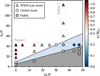Fig. 9. Instability diagram showing the resistive wavenumber, kη, as a function of the stratification wavenumber, kN, both scaled by the shell gap, D. Individual simulation runs are represented by symbols: crosses indicate decaying nonaxisymmetric perturbations, while circles and triangles mark unstable global and WKB-type m = 1 modes, respectively. The symbol color codes the instability growth rate σ. The shaded gray and blue regions denote the stable regime and the global mode regime, respectively, based on the simulation data. The boundaries of these shaded regions are defined by Eq. (43) (stability line) and Eq. (44) (transition line between the global and WKB regimes). Thin dotted horizontal and vertical rectangles highlight runs in subset 1 (${\overline{\mathrm{Lu}}}_1\approx 680$) and subset 2 (${\overline{\delta }}_1=180$).

$$\begin{array}{c}\hfill k_{\eta }D=5.22+0.71k_{N}D.\end{array}$$(43)

This equation defines the boundary of the shaded gray region in the figure. It is important to note that this relationship, with its distinct offset and slope, deviates from the marginal stability line k_η = k_N predicted by the local linear theory.

Triangles and circles in Fig. 9 represent simulation runs where the perturbations exhibit exponential growth. Specifically, triangles denote unstable fluctuations resembling WKB modes, while circles correspond to the global equatorial modes identified in our linear analysis, as we shall discuss further. In all these runs, the m = 1 azimuthal mode is the first to grow exponentially after introducing the perturbations, similar to the reference unstratified case TU0 (Sect. 3.4.1). Higher azimuthal modes display analogous dynamical evolutions to those observed in run TU0 and are thus not discussed here. Far from the instability threshold, where k_η ≫ k_N and resistive effects are negligible, the growth rates of the m = 1 mode, indicated by the symbol color in Fig. 9, are consistent with $\sigma \approx {\overline{\omega }}_{\mathrm{A}1}$, which aligns with the WKB prediction. Throughout this section, σ was calculated from the temporal evolution of the volume-averaged toroidal magnetic energy associated with the m = 1 mode, as is described in Sect. 3.4.1.

Due to their lower growth rates, global modes primarily become apparent in the simulations when approaching the stable regime; that is, when resistive effects begin to damp the small-scale WKB modes. The transition line between the WKB and global mode regimes, derived from the simulation data, is

$$\begin{array}{c}\hfill k_{\eta }D=9.01+1.12k_{N}D,\end{array}$$(44)

which defines the upper boundary of the shaded blue region in Fig. 9.

We now explore how the properties of the Tayler modes identified in the simulations change from the WKB to the global mode regime by following two distinct paths in the parameter space. The first path fixes the resistive wavenumber at k_η ≈ 42/D (or ${\overline{\mathrm{Lu}}}_1\approx 680$) and gradually increases k_N by varying the stratification parameter ${\overline{\delta }}_1$. The simulation runs for this first path, hereafter referred to as subset 1, are enclosed by the thin horizontal rectangle in Fig. 9. The second path toward the global mode regime is defined by a fixed k_N = 35/D (or ${\overline{\delta }}_1=180$) and a decreasing k_η, achieved by varying the Lundquist number ${\overline{\mathrm{Lu}}}_1$. Runs belonging to this second path are designated as subset 2 (thin vertical rectangle in Fig. 9).

For subset 1 runs with k_N ≤ 25/D (or ${\overline{\delta }}_1\le 90$), the instability growth rate is close to the adiabatic one with $\sigma \gtrsim 0.4{\overline{\omega }}_{\mathrm{A}1}$ (triangles in the horizontal rectangle of Fig. 9; see also Table 1). The magnetic field fluctuations are localized from high to intermediate latitudes, in a wedge-shaped region around the vertical symmetry axis, as expected for WKB modes (Fig. 11a–c). For each of these runs, we estimated the characteristic radial wavenumber of the instability, k_r, from a snapshot of ${\stackrel{\sim }{B}}_{\theta }\prime$ taken during the linear growth phase. Specifically, we computed k_r = π/λ_r, where λ_r is the characteristic half-wavelength, determined as the mode of the distribution of distances between two successive nodes in the radial profiles of ${\stackrel{\sim }{B}}_{\theta }\prime$, measured at a colatitude θ = 30° and for all longitudes. The wavenumbers observed in these runs consistently fall within the theoretical WKB limits (k_N <  k_r <  k_η) and, as was expected, increase with stratification, as is demonstrated by Fig. 10a (triangles).

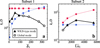Fig. 10. Comparison of the radial wavenumbers, kr, observed in the numerical simulation runs of (a) subset 1 and (b) subset 2 (triangles and circles; see also Fig. 9) with the WKB predictions. Blue and red squares show, respectively, the minimum (kN) and maximum (kη) unstable wavenumbers as predicted by the WKB theory (Eqs. (41) and (42)).

As ${\overline{\delta }}_1$ increases to 130, where k_ηD is only about 1.3 k_ND, resistive effects begin to dampen the WKB modes. We identify a new class of unstable m = 1 fluctuations which, unlike the previous WKB-type modes, are nearly constant in latitude and start also to be active in the equatorial region (Fig. 11d). The growth rate of these modes reduces to $0.28{\overline{\omega }}_{\mathrm{A}1}$ and their radial wavenumber is k_r ≈ 25/D, which falls below the minimum wavenumber of k_N ≈ 30/D predicted by the local linear theory (Fig. 10a). Further increasing ${\overline{\delta }}_1$ leads to fluctuations with consistently lower growth rates (circles in subset 1 runs of Fig. 9) and increasingly larger radial length scales (Fig. 11e,f), which further deviate from the theoretical WKB predictions (Fig. 10a, circles). These findings align with our linear analysis, as the global equatorial eigenmodes also display large radial length scales and growth rates that diminish with stable stratification (Sect. 2.2.2).

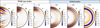Fig. 11. Meridional slices of the nonaxisymmetric latitudinal magnetic field, ${\stackrel{\sim }{B}}_{\theta }\prime$, during the linear growth phase of the instability for six simulation runs of subset 1 in Fig. 9, spanning different values of the stratification parameter ${\overline{\delta }}_1$. WKB-type modes are identified for ${\overline{\delta }}_1\le 54$, while global modes emerge for ${\overline{\delta }}_1\ge 130$. The leftmost panel corresponds to the unstratified run TU0 described in Sect. 3.4.1.

Simulation runs in subset 2 at ${\overline{\delta }}_1=180$ (vertical rectangle in Fig. 9) exhibit analogous behavior when moving toward the global mode regime by decreasing the Lundquist number. At the largest ${\overline{\mathrm{Lu}}}_1$ of 5481 explored (or k_η = 121/D) the instability growth rate is near adiabatic, with $\sigma =0.85{\overline{\omega }}_{\mathrm{A}1}$. The magnetic fluctuations are concentrated at high latitudes (not shown) and are small-scale, with a characteristic radial wavenumber of k_r = 45/D, falling within the expected WKB limits (Fig. 10b). As ${\overline{\mathrm{Lu}}}_1$ decreases, k_r progressively declines within the range of unstable WKB wavenumbers, until global modes emerge at the lowest ${\overline{\mathrm{Lu}}}_1$ of 680 (circle in Fig. 10b).

Finally, we detail the variation in the instability growth rate with stratification, focusing on the simulation runs in subset 1. Figure 12 presents the square of the normalized growth rate, ${\mathrm{\Gamma }}^2={\sigma }^2/{\overline{\omega }}_{\mathrm{A}1}^2$, as a function of ${\overline{\delta }}_1^2$ for these runs. For ${\overline{\delta }}_1^2\lesssim {10}^3$, where stratification is weak, the growth rate Γ only slightly decreases from the adiabatic value of 1 observed in the unstratified run TU0. In this regime, as previously demonstrated, we clearly identified WKB-like modes (Fig. 10a). At intermediate values of the stratification parameter, ${10}^3<{\overline{\delta }}_1^2<{10}^4$, we find stronger variations in the growth rate, yet still identify WKB-like modes. A power law fit ${\mathrm{\Gamma }}^2=c{\overline{\delta }}_1^{2b}$ to the simulation data points in this stratification range yields c = 71 and an exponent b = −0.66. This fit is shown as a dotted line in Fig. 12. The value of b is close to the one found in the numerical simulations of Guerrero et al. (2019), which is −0.95, suggesting that their study focused on WKB-type Tayler modes.

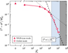Fig. 12. Square of the normalized instability growth rate, Γ2, as a function of ${\overline{\delta }}_1^2$ for the simulation runs of subset 1 (see Fig. 9). The dashed line shows the best-fit power law for runs in the global mode regime (${\overline{\delta }}_1^2>{10}^4$; circles): ${\mathrm{\Gamma }}^2\propto 1/{\overline{\delta }}_1^{4.1}$. The dotted line indicates the best fit for runs in the moderately stratified regime with WKB-type modes (triangles in the range ${10}^3<{\overline{\delta }}_1^2<{10}^4$): ${\mathrm{\Gamma }}^2\propto 1/{\overline{\delta }}_1^{1.3}$. The shaded gray and blue areas mark, respectively, the stable and global mode regimes as identified in Fig. 9. The thick horizontal bars associated with each data point indicate the range of ${\overline{\delta }}_1$ values attained during the linear phase of the instability growth (see text for details). For the unstratified case and the first five stratified runs, these bars are smaller than the symbol size.

For ${\overline{\delta }}_1^2>{10}^4$, where global modes are identified, the best fitting parameters are c = 4.07 × 10⁷ and b = −2.05 (dashed line in Fig. 12). This value of b is in excellent agreement with the prediction by BU12, which is also confirmed by our linear analysis in Sect. 2.2.2. In this regime, the instability grows at such a low rate that the amplitude of the background axisymmetric field $⟨{\stackrel{\sim }{B}}_{\varphi }⟩$ decreases during the linear evolution of the instability, thereby leading to an increase in ${\overline{\delta }}_1$ over time. The thick horizontal bars associated with the data points in Fig. 12 indicate the range of values of ${\overline{\delta }}_1$ attained during the entire linear phase of the instability, and demonstrate that such variations do not impact the growth rate scaling.

In summary, our numerical simulations provide a comprehensive understanding of the Tayler instability in spherical geometry, confirming and extending the results of the global linear analysis. We successfully reproduce modes known from the WKB approximation and, in the regime where resistive effects suppress these, reveal a distinct class of large-scale fluctuations which exhibit key similarities with the global equatorial eigenmodes identified in the linear analysis.

4. Application to red giant cores

Our direct numerical simulations uncovered two regimes for the nonaxisymmetric Tayler instability. The first is characterized by unstable modes localized at high to intermediate latitudes, with fast growth rates and small radial length scales, which are also accessible to the WKB approximation. The second regime consists of global modes, extending in the equatorial region and exhibiting reduced growth rates and large radial length scales. This latter regime lies adjacent to the region of the parameter space (k_N, k_η) where no instability is found. The stability line given by Eq. (43), derived from our numerical simulation results, can be recast as a cubic polynomial equation,

$$\begin{array}{c}\hfill x^3-a_1{\mathcal{A}}_{1}x-a_0{\mathcal{A}}_0=0,\end{array}$$(45)

where x = B_ϕ^1/4. The coefficients are a₀ = 0.71 and a₁ = 5.22, and the functions 𝒜₀ and 𝒜₁ are defined by

$$\begin{array}{c}\hfill {\mathcal{A}}_0={(4\pi \rho )}^{3/8}{(N\eta )}^{1/2}{\kappa }^{-1/4}{R}^{1/4}\end{array}$$(46)

and

$$\begin{array}{c}\hfill {\mathcal{A}}_1={(4\pi \rho )}^{1/4}{\eta }^{1/2}{R}^{-1/2}.\end{array}$$(47)

All quantities are expressed in cgs units, and R denotes the radial extent of the radiative region. The solution to this equation yields the critical toroidal field strength for instability onset, B_crit, above which the global modes become the dominant unstable fluctuations.

An analogous equation can be obtained for the transition line between the global mode regime and the regime of WKB-type modes (Eq. (44)). In this case, the coefficients are a₀ = 1.12 and a₁ = 9.01, and its solution provides the transition toroidal field strength, B_trans. For a given star, the knowledge of the size of its radiative region, R, together with radial profiles of the density, ρ, thermal Brunt-Väisälä frequency, N, thermal diffusivity, κ, and magnetic diffusivity, η, therein, allows us to predict these two threshold field strengths.

To estimate B_crit and B_trans, we computed stellar evolution models of two stars with initial masses of 1.1 and 1.5 M_⊙, where M_⊙ is the mass of the Sun. These models span the mass range of SGs and red giants for which internal magnetic fields are detected (Sect. 1). We evolved both stars from the zero age main sequence up to the RGB using the Catania version of the Garching Stellar Evolution Code (Weiss & Schlattl 2008; Bonanno et al. 2002), reaching final ages of 10.53 and 3.34 Gyr for the 1.1 and 1.5 M_⊙ stars, respectively. We assumed an initial hydrogen and helium mass fraction of X = 0.70 and Y = 0.27, respectively. No heavy-element diffusion was included and we chose a mixing-length parameter α_MLT = 1.65, obtained from solar calibration. For each stellar mass, we selected two models: one in the SG phase and one at the base of the RGB. Since we found no significant difference in our estimates of B_crit and B_trans for the two stellar masses, we discuss only the results for the 1.1 M_⊙ star in the following. For this star, the SG (RGB) model has an age of 10.127 (10.489) Gyr, a radius of R_*/R_⊙ = 3.2 (16.1), and a luminosity of L_*/L_⊙ = 4.6 (70.1), where R_⊙ and L_⊙ are the radius and luminosity of the present-day Sun, respectively.

We calculated the thermal diffusivity κ as (e.g., Cassisi et al. 2007)

$$\begin{array}{c}\hfill \kappa =\frac{16{\sigma }_{\mathrm{B}}{T}^3}{3k{\rho }^2{c}_p},\end{array}$$(48)

where σ_B is the Stefan-Boltzmann constant, c_p is the specific heat capacity at constant pressure, and k is the total opacity. The total opacity is defined by $k^{-1}=k_{\mathrm{rad}}^{-1}+k_{\mathrm{cond}}^{-1}$, with k_rad and k_cond being the radiative and conductive opacities, respectively, as computed in GARSTEC (see Weiss & Schlattl 2008). The magnetic diffusivity, η, was computed using standard expressions detailed in Appendix A, which account for the collisional contribution from Spitzer conductivity in the outer, nondegenerate regions of the core, and for electron degeneracy effects in the inner layers.

Figure 13a presents the radial profiles of the thermal contribution to the squared Brunt-Väisälä frequency (N²), density (ρ), thermal diffusivity (κ), and magnetic diffusivity (η) within the radiative cores of the SG (black lines) and RGB (red lines) stars. These profiles extend up to the lower part of the convective envelopes (N² <  0, indicated by the shaded gray regions with dotted hatching). For each star, hydrogen burning takes place within a narrow shell, the hydrogen-burning shell (HBS). Its approximate location is indicated by the vertical dotted line, which coincides with the luminosity jump and aligns with the peak in N² (solid line). The regions of the core below the HBS are composed of inert helium. Here, N² increases by about an order of magnitude from the SG to the RGB stage, primarily due to the rise in density (dashed lines) driven by the core gravitational contraction. In these inner regions, the density reaches up to 10⁵ g/cm³, and heat transport is dominated by electron conduction. In contrast, in the core regions above the HBS, heat is primarily transported by radiation. The steep density drop across the HBS leads to an increase in thermal diffusivity κ (dash-dotted lines) by more than four orders of magnitude in this region. For both stellar stages, η remains low – between 0.1 and 1 cm²/s – in the inner degenerate core regions due to the high conductivity of the electron gas, and rises to 10² − 10³ cm²/s in the outer, nondegenerate parts of the core (dotted lines).

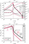Fig. 13. Radial profiles of (a) key stellar quantities and (b) threshold toroidal field strengths for the 1.1 M⊙ stellar model at SG (black lines) and RGB (red lines) stages. The profiles span the radiative cores and the lower parts of the convective envelopes (vertical gray dot-hatched regions). Vertical dotted lines mark the approximate locations of the HBS. The upper horizontal axis shows the radius, r, in units of the solar radius, R⊙; the surface radii are 3.2 R⊙ (SG) and 16.1 R⊙ (red giant). Panel (a) displays the thermal contribution to the squared Brunt-Väisälä frequency (N2; right axis), along with the density, ρ, thermal diffusivity, κ, and magnetic diffusivity, η (left axis). Panel (b) shows the critical toroidal field strength for instability onset, Bcrit (solid lines) and the transition field strength, Btrans (dotted lines), which marks the boundary between the global and WKB-type instability regimes. The shaded regions between the two curves indicate the range of field strengths where global modes are expected. The vertical shaded region near the HBS of each star highlights the region where the chemical contribution to the Brunt-Väisälä frequency, Nμ, becomes significant compared to the thermal one, i.e., where |Nμ|> N/2.

Figure 13b displays B_crit (solid lines) and B_trans (dotted lines) as a function of radius for the SG and RGB stars. Toroidal fields with strengths of B_ϕ <  B_crit are stable. In the degenerate core regions below the HBS, the profiles of B_crit are nearly identical for the two stars. They increase monotonically from 6 kG in the innermost parts to about 50 kG as they approach the HBS. Just below the HBS, B_crit drops sharply and continues to decline in the outer core regions, reaching values of a few gauss or less near the base of the convection zone. We caution that our analysis does not strictly apply in a narrow region in the vicinity of the HBS, where chemical stratification – neglected here – becomes comparable to or stronger than thermal stratification (see vertical shaded gray and red regions in Fig. 13b).

Global Tayler modes develop within a limited range of field strengths, specifically where B_crit <  B_ϕ ≤ B_trans (shaded gray and red areas between the solid and dotted curves in Fig. 13b). Our numerical simulations and linear analysis confirm the relation of BU12 for the growth rate of the global modes,

$$\begin{array}{c}\hfill \mathrm{\Gamma }\propto ϵ{\delta }^{-2},\end{array}$$(49)

or, in cgs units,

$$\begin{array}{c}\hfill \sigma \propto \frac{B_{\varphi }^2\kappa }{4\pi \rho R^4{N}^2}.\end{array}$$(50)

Here, we adopted the definitions from Sect. 2.2, with R denoting the characteristic radial extent of the unstable region within the core where global modes operate. The proportionality factor in Eq. (49) is determined from the numerical simulations of subset 1 (see Fig. 12 and the corresponding discussion). The e-folding time of these modes, τ = σ⁻¹, varies significantly across the radiative core and depends sensitively on R, which itself reflects the evolutionary stage. For instance, assuming R = 10⁹ cm, τ remains several orders of magnitude higher than the typical core evolution timescale (hundreds of Myr for SGs and tens of Myr on the RGB) in regions below the HBS, rendering global modes dynamically irrelevant there. However, in the outer core layers where stratification is weaker, τ becomes comparable to evolutionary timescales, indicating that global modes may have dynamical impact.

The radial profiles of B_trans for the two stellar stages broadly follow those of the critical field strengths discussed above, but with systematically higher amplitudes (Fig. 13b, dotted lines). Below the HBS, B_trans ranges between 10 and 100 kG for both stellar stages. Above the HBS, B_trans decreases monotonically with radius to values on the order of 1 G or below near the base of the convection zone. Dynamical impact on the core is expected in the regime of WKB-type modes, corresponding to toroidal field strengths exceeding B_trans. These modes grow at Alfvénic rates, corresponding to core Afvén travel times of 10² − 10³ years for field strengths near B_trans.

5. Summary and conclusions

We first investigated the current-driven nonaxisymmetric (m = 1) Tayler instability in a spherical domain using a linear stability analysis that is global in radius. This analysis accounts for stable thermal stratification and thermal diffusion, and extends the work of Bonanno & Urpin (2012) by including the latitudinal structure of the background toroidal field. The background toroidal field is in magnetohydrostatic equilibrium, with gravitational, pressure, and Lorentz forces in balance, as is expected in radiative stellar interiors. Our global approach captures the full radial structure of the unstable m = 1 perturbations, a feature inaccessible to fully local analyses (Acheson & Gibbons 1978; Spruit 1999; Skoutnev & Beloborodov 2024), and demonstrates the stabilizing influence of gravity on these perturbations.

Next, we used the same background toroidal field to study the Tayler instability through 3D direct numerical simulations in a nearly full-sphere geometry, tracking its evolution from the linear to the nonlinear phase. Unlike previous studies in a similar geometry (Guerrero et al. 2019; Monteiro et al. 2023), our simulations systematically explore the effect of thermal stratification on the instability, including the influence of finite viscosity and magnetic resistivity. The numerical simulations revealed two distinct instability regimes, each characterized by a different class of nonaxisymmetric fluctuations. The simulations also allowed us to derive empirical laws for both the critical toroidal field strength for instability onset and the transition field strength separating the two instability regimes, expressed in terms of fundamental stellar fluid properties.

In the highly supercritical regime where viscous and resistive effects are negligible, both the linear analysis and the numerical simulations confirm previous results from local analyses in the WKB approximation. The most unstable modes in this regime are confined between mid to high latitudes, forming a wedge-shaped region around the vertical symmetry axis of the background toroidal field. As the stratification parameter, δ (defined as the ratio of the Brunt-Väisälä frequency, N, to the Alfvén frequency of the background toroidal field, ω_A0) increases, the radial wavenumber of these modes grows. Their growth rate, however, remains on the order of ω_A0, as is expected.

In the equatorial region, our linear analysis unveils a new class of unstable modes, inaccessible to a fully local approach, characterized by large radial length scales and reduced growth rates. The numerical simulations demonstrate that these global modes dominate the dynamics when the system approaches the stability line, specifically when viscous and resistive effects start to dampen the high-latitude WKB-type modes. Both our linear analysis and, for the first time, our numerical simulations confirm that the dimensionless growth rate of the global equatorial modes follows a scaling of Γ ∼ δ⁻², or equivalently, in dimensional quantities, σ ∼ ω_A0³/N², as was anticipated by BU12.

Our results provide a general framework for evaluating the linear stability of toroidal magnetic fields within radiative stellar interiors. From our numerical simulations, we established two straightforward algebraic equations (Eqs. (45)–(47)) relating the critical toroidal field strength for the instability onset, B_crit, and the transition field strength, B_trans, which separates the unstable regimes where global and WKB-type modes dominate, to internal fluid properties readily available from stellar evolutionmodels.

We computed stellar evolution models for 1.1 and 1.5 M_⊙ stars and selected two evolutionary stages for each star: the early SG phase and the base of the RGB. These models provided radial profiles of the Brunt-Väisälä frequency, N, density, ρ, and thermal diffusivity, κ, in the radiative core. We also estimated the magnetic diffusivity, η, in both the outer nondegenerate and inner degenerate regions of the core.

For both stellar masses, the degenerate core regions below the HBS show B_crit ranging from 6 to 50 kG and B_trans from 10 to 100 kG, with little variation between the two evolutionary stages. Both threshold field strengths drop sharply – by over two orders of magnitude – across the HBS and continue to decline outward to values below 1 G. This trend suggests that the outer regions of SG and red giant cores are likely to host unstable toroidal fields. We recall that these results apply in the limit of slow rotation, i.e., when the rotation rate, Ω, is much smaller than ω_A0 locally, as the stabilizing influence of the Coriolis force on the instability (e.g., Spruit 1999) was not taken into account.

Recent asteroseismic studies suggest that axisymmetric toroidal fields may dominate, though not overwhelmingly, over the detected radial magnetic fields in the cores of SGs and red giants (Li et al. 2022; Deheuvels et al. 2023; Li et al. 2023). However, detecting such toroidal fields remains challenging, as asteroseismic inversion kernels exhibit limited sensitivity to them, at least for the background configurations explored to date (Bhattacharya et al. 2024). Broader investigations of alternative field configurations are needed to clarify the detectability of toroidal fields using mixed oscillation modes. Despite these limitations, the threshold toroidal field strengths derived here offer valuable constraints for future asteroseismic studies, particularly in core regions where rotation plays aminor role.

We emphasize that our results apply to radiative interiors across a wide range of stellar masses and evolutionary stages. For the core of the present-day Sun, for instance, the Brunt-Väisälä frequency is approximately N = 10⁻³ s⁻¹, with thermal and magnetic diffusivities of κ ∼ 10⁸ cm²/s and η ∼ 10³ cm²/s, respectively. Using our scaling relations, we estimate a critical field strength of B_crit ∼ 10 G and a transitional strength of B_trans ∼ 10² G.

While a detailed characterization of the nonlinear solutions is left to future work, our simulations already provide an insight into the resulting magnetic field geometries. In the global mode regime, the field evolves toward a simple, large-scale configuration dominated by the axisymmetric toroidal component. This is because the nonaxisymmetric field fluctuations grow so slowly that the background toroidal field decays resistively before reaching the nonlinear stage, and the axisymmetric poloidal field generated by the instability remains negligible. In contrast, in the regime of WKB-type modes, the instability generally produces turbulent field solutions with mixed poloidal-toroidal character, owing to flow and field fluctuations growing at a faster Alfvén rate. In our most strongly stratified and supercritical run (TS12; see Table 1), the ratio of the RMS axisymmetric poloidal to toroidal field reaches about 10⁻² in the nonlinear phase.

In this study, we have not addressed the effect of rotation on the instability, leaving this important aspect for future work. While local perturbation analyses indicate that the Coriolis force generally reduces the growth rate of the Tayler instability compared to the nonrotating case (Pitts & Tayler 1985; Spruit 1999; Skoutnev & Beloborodov 2024), a comprehensive understanding of the instability and the resulting turbulent transport under the combined influences of rotation, differential rotation, and both chemical and thermal stratification – all relevant to stellar interiors – is lacking. Nonetheless, progress has recently begun in this direction. A local linear analysis incorporated the effects of rotation and of both thermal and compositional stratification in spherical geometry (Skoutnev & Beloborodov 2025), while current numerical efforts are devoted to testing the scaling predictions for turbulent transport derived from order-of-magnitude estimates of the instability saturation (Petitdemange et al. 2023; Barrère et al. 2023, 2025). Extending numerical simulations to strongly stratified regimes, as has been initiated in this work, together with global linear stability analyses such as the one presented here, is crucial for understanding the saturation mechanism of the Tayler instability and accurately quantifying the associated turbulent transport.

Acknowledgments

The authors thank the anonymous reviewer for their insightful and constructive comments that improved the manuscript. This research was funded by the Deutsche Forschungsgemeinschaft (DFG, German Research Foundation) – AR 355/13-1, within the framework of “Stability and generation of magnetic fields in red giants: towards a unified picture”. DGM acknowledges support from the European Union – NextGenerationEU under the Italian National Recovery and Resilience Plan (NRRP), Mission 4: Education and Research, Component M4C2, Investment 1.2, through the “Avviso Young Researchers 2024”, Project No. SOE2024_0000097, “Elucidating the Transport of Angular momentum by MAgnetic fields in red GIAnts (ETAMAGIA)”. AB acknowledges support from the European Union – NextGenerationEU RRF M4C2 1.1 No. 2022HY2NSX “CHRONOS: adjusting the clock(s) to unveil the CHRONO-chemo-dynamical Structure of the Galaxy”. AB and GL acknowledge support from the research grant “Unveiling the magnetic side of the Stars” funded under the INAF national call for Fundamental Research 2023.

References

Appendix A: Microscopic magnetic diffusivity

The magnetic diffusivity in red giant cores was computed using standard expressions detailed below. We define the magnetic diffusivity, η, as

$$\begin{array}{c}\hfill \eta =\frac{c^2}{4\pi ({\sigma }_{\mathrm{coll}}+{\sigma }_{\mathrm{e}})},\end{array}$$(A.1)

where c is the speed of light, and σ_coll and σ_e denote the contributions to the electrical conductivity from collisional processes and electron degeneracy, respectively. For σ_coll, which dominates over σ_e in the core regions above the HBS, we adopt the classical expression for the electrical conductivity of a nondegenerate, fully ionized, ideal gas of Spitzer (1962)

$$\begin{array}{c}\hfill {\sigma }_{\mathrm{coll}}={\gamma }_{\mathrm{E}}\frac{2{(2k_{\mathrm{B}}T)}^{3/2}}{{\pi }^{3/2}{m}_{\mathrm{e}}^{1/2}Z{e}^{2}ln\mathrm{\Lambda }},\end{array}$$(A.2)

where k_B is the Boltzmann constant, T is temperature, m_e is the electron mass, Z is the atomic number, e is the electron charge, lnΛ is the Coulomb logarithm, and γ_E is the correction for electron-electron scattering which we set to 0.582 for a pure hydrogen plasma (Wendell et al. 1987).

Below the HBS in red giant cores, electron degeneracy becomes significant and transport processes are governed by electron conduction (Garaud et al. 2015). The electrical conductivity is dominated by the degenerate electron contribution σ_e here, for which we adopt the expressions derived by Hubbard (1966) for a strongly degenerate electron gas. The corresponding thermal conductivity K is given by

$$\begin{array}{c}\hfill K=\frac{{(2\pi ħ)}^3{k}_{\mathrm{B}}^2}{16m_{\mathrm{e}}^2{e}^{4}A{m}_{\mathrm{H}}}{G}_{\gamma }({\kappa }_{\mathrm{F}})\rho T,\end{array}$$(A.3)

where ℏ is the reduced Planck constant, ρ is density, A is the average atomic number of the nuclei, m_H is the mass of the hydrogen atom, and κ_F = (9πZ/4)^1/3 is the dimensionless Fermi wavenumber. The function G_γ is

$$\begin{array}{c}\hfill G_{\gamma }(x)=\frac{1}{ln(1+4x^2/3\gamma )},\end{array}$$(A.4)

where γ is the dimensionless parameter

$$\begin{array}{c}\hfill \gamma =\frac{Z^2{e}^2}{k_{\mathrm{B}}T}{\left(\frac{4\pi \rho }{3A{m}_{\mathrm{H}}}\right)}^{1/3}.\end{array}$$(A.5)

Since the degenerate red giant core regions are mostly composed of helium, we used A = 4 and Z = 2 in Eqs. (A.3) and (A.5). In the limit of high degeneracy, the Wiedemann-Franz law holds,

$$\begin{array}{c}\hfill K=\frac{1}{3}{\pi }^2{k}_{\mathrm{B}}^2{\sigma }_{\mathrm{e}}T/e^2,\end{array}$$(A.6)

which we used to determine σ_e from K. In the region of weak electron degeneracy around the HBS, where neither the expression for σ_e nor the one for σ_coll is strictly applicable, we estimated η using a cubic spline interpolation between the degenerate contribution from the deeper core and the collisional contribution from the outer core.

All Tables

All Figures

Fig. 1. Radial profiles of the real parts of selected unstable latitudinal field eigenmodes, Re(Bθ′), in the absence of thermal diffusion (ϵ = 0). Panels (a)–(c) show the high-latitude eigenmodes (θ = 5°) with the nearly adiabatic growth rate of Γ = 0.95 for different values of the stratification parameter δ (see legend insets). The inset in (c) provides a zoom on the eigenmode between r = 0.10 and 0.12. Panel (d) displays the most unstable eigenmodes at the equator (θ = 90°); no unstable modes are found for δ ≥ 25. The horizontal axis is logarithmic in (a)–(c) and linear in (d).

In the text

Fig. 2. Radial wavenumber, kr, of various unstable eigenmodes, evaluated from the real part of Bθ′, as a function of δ for (a) no thermal diffusion (ϵ = 0) and (b) finite thermal diffusion (ϵ = 10−2). Triangles connected by solid lines indicate eigenmodes at colatitude θ = 5° with growth rates Γ = 0.8 (blue), 0.9 (purple), and 0.95 (red). Selected eigenmodes of the Γ = 0.95 tracks in (a) and (b) are displayed in Figs. 1a–c and 3a–c, respectively. The dotted lines denote the minimum unstable wavenumber predicted by the local linear theory (Eqs. (19) and (21)). Open gray circles connected by dashed lines correspond to the equatorial eigenmodes (Fig. 1d and dashed lines in Fig. 3d).

In the text

	Fig. 3. Same as Fig. 1 but for ϵ = 10−2. In panel (d), dashed and solid lines correspond to the type I and type II equatorial eigenmodes, respectively (see text for details). Type I eigenmodes are the most unstable (see Fig. 4 for their growth rate values). The horizontal axis is logarithmic in all panels.
In the text

	Fig. 4. Dimensionless growth rates of the type I equatorial eigenmodes, Γmax, as a function of the stratification parameter δ for ϵ = 10−2. The dashed line indicates the scaling predicted by Bonanno & Urpin (2012), Γmax ∝ δ−2.
In the text

	Fig. 5. Temporal evolution of the volume integrated toroidal magnetic energy (black lines) and poloidal kinetic energy (red lines). Results are shown for the unstratified run (δ0 = 0) and two stratified runs (δ0 = 300 and 900). The Lundquist number is Lu0 = 917. Both the flow and magnetic field remain purely axisymmetric throughout the evolution.
In the text

Fig. 6. Snapshots of the three axisymmetric simulation runs presented in Fig. 5. Snapshot times tωA0 are 26.6 for (a) δ0 = 0, 26.9 for (b) δ0 = 300, and 27.3 for (c) δ0 = 900. Color contours show the axisymmetric azimuthal field, $⟨{\stackrel{\sim }{B}}_{\varphi }⟩$. Black contour lines represent the meridional circulation, with solid and dashed lines indicating clockwise and counterclockwise flows, respectively.

In the text

Fig. 7. Temporal evolution of the (a) toroidal and (b) poloidal magnetic energies for the azimuthal modes m = 0 to m = 6 in the unstratified run TU0. The dashed black lines show exponential fits to the energy evolution of the m = 1 mode within the time interval $6.5\le (t-t_1){\overline{\omega }}_{\mathrm{A}1}\le 10.5$. These fits are used to determine the instability growth rates σ discussed in the text.

In the text

Fig. 8. Snapshots of the magnetic field fluctuations and axisymmetric field for the unstratified run TU0. The three leftmost, middle, and rightmost panels show the linear stage of the instability, the end of the linear stage, and the nonlinear stage, respectively. (a–c) Hammer projections of the nonaxisymmetric latitudinal field ${\stackrel{\sim }{B}}_{\theta }\prime$ at radius r/rout = 0.7. (d,f,h) Meridional slices of ${\stackrel{\sim }{B}}_{\theta }\prime$ at longitude ϕ = 90°. (e,g,i) Color isocontours depict the axisymmetric azimuthal field, $⟨{\stackrel{\sim }{B}}_{\varphi }⟩$, with overlaid black contour lines indicating the axisymmetric poloidal field.

In the text

Fig. 9. Instability diagram showing the resistive wavenumber, kη, as a function of the stratification wavenumber, kN, both scaled by the shell gap, D. Individual simulation runs are represented by symbols: crosses indicate decaying nonaxisymmetric perturbations, while circles and triangles mark unstable global and WKB-type m = 1 modes, respectively. The symbol color codes the instability growth rate σ. The shaded gray and blue regions denote the stable regime and the global mode regime, respectively, based on the simulation data. The boundaries of these shaded regions are defined by Eq. (43) (stability line) and Eq. (44) (transition line between the global and WKB regimes). Thin dotted horizontal and vertical rectangles highlight runs in subset 1 (${\overline{\mathrm{Lu}}}_1\approx 680$) and subset 2 (${\overline{\delta }}_1=180$).

In the text

	Fig. 10. Comparison of the radial wavenumbers, kr, observed in the numerical simulation runs of (a) subset 1 and (b) subset 2 (triangles and circles; see also Fig. 9) with the WKB predictions. Blue and red squares show, respectively, the minimum (kN) and maximum (kη) unstable wavenumbers as predicted by the WKB theory (Eqs. (41) and (42)).
In the text

Fig. 11. Meridional slices of the nonaxisymmetric latitudinal magnetic field, ${\stackrel{\sim }{B}}_{\theta }\prime$, during the linear growth phase of the instability for six simulation runs of subset 1 in Fig. 9, spanning different values of the stratification parameter ${\overline{\delta }}_1$. WKB-type modes are identified for ${\overline{\delta }}_1\le 54$, while global modes emerge for ${\overline{\delta }}_1\ge 130$. The leftmost panel corresponds to the unstratified run TU0 described in Sect. 3.4.1.

In the text

Fig. 12. Square of the normalized instability growth rate, Γ2, as a function of ${\overline{\delta }}_1^2$ for the simulation runs of subset 1 (see Fig. 9). The dashed line shows the best-fit power law for runs in the global mode regime (${\overline{\delta }}_1^2>{10}^4$; circles): ${\mathrm{\Gamma }}^2\propto 1/{\overline{\delta }}_1^{4.1}$. The dotted line indicates the best fit for runs in the moderately stratified regime with WKB-type modes (triangles in the range ${10}^3<{\overline{\delta }}_1^2<{10}^4$): ${\mathrm{\Gamma }}^2\propto 1/{\overline{\delta }}_1^{1.3}$. The shaded gray and blue areas mark, respectively, the stable and global mode regimes as identified in Fig. 9. The thick horizontal bars associated with each data point indicate the range of ${\overline{\delta }}_1$ values attained during the linear phase of the instability growth (see text for details). For the unstratified case and the first five stratified runs, these bars are smaller than the symbol size.

In the text

Fig. 13. Radial profiles of (a) key stellar quantities and (b) threshold toroidal field strengths for the 1.1 M⊙ stellar model at SG (black lines) and RGB (red lines) stages. The profiles span the radiative cores and the lower parts of the convective envelopes (vertical gray dot-hatched regions). Vertical dotted lines mark the approximate locations of the HBS. The upper horizontal axis shows the radius, r, in units of the solar radius, R⊙; the surface radii are 3.2 R⊙ (SG) and 16.1 R⊙ (red giant). Panel (a) displays the thermal contribution to the squared Brunt-Väisälä frequency (N2; right axis), along with the density, ρ, thermal diffusivity, κ, and magnetic diffusivity, η (left axis). Panel (b) shows the critical toroidal field strength for instability onset, Bcrit (solid lines) and the transition field strength, Btrans (dotted lines), which marks the boundary between the global and WKB-type instability regimes. The shaded regions between the two curves indicate the range of field strengths where global modes are expected. The vertical shaded region near the HBS of each star highlights the region where the chemical contribution to the Brunt-Väisälä frequency, Nμ, becomes significant compared to the thermal one, i.e., where |Nμ|> N/2.

In the text

References

- Acheson, D. J., & Gibbons, M. P. 1978, Phil. Trans. R. Soc. Lond. A, 289, 459 [Google Scholar]
- Arlt, R., & Rüdiger, G. 2011, Astron. Nachr., 332, 70 [NASA ADS] [CrossRef] [Google Scholar]
- Balbus, S. A., & Hawley, J. F. 1991, ApJ, 376, 214 [Google Scholar]
- Barrère, P., Guilet, J., Raynaud, R., & Reboul-Salze, A. 2023, MNRAS, 526, L88 [CrossRef] [Google Scholar]
- Barrère, P., Guilet, J., Raynaud, R., & Reboul-Salze, A. 2025, A&A, 695, A183 [NASA ADS] [CrossRef] [EDP Sciences] [Google Scholar]
- Bhattacharya, S., Das, S. B., Bugnet, L., Panda, S., & Hanasoge, S. M. 2024, ApJ, 970, 42 [NASA ADS] [CrossRef] [Google Scholar]
- Bonanno, A., & Urpin, V. 2008, A&A, 477, 35 [NASA ADS] [CrossRef] [EDP Sciences] [Google Scholar]
- Bonanno, A., & Urpin, V. 2011, Phys. Rev. E, 84, 056310 [Google Scholar]
- Bonanno, A., & Urpin, V. 2012, ApJ, 747, 137 [NASA ADS] [CrossRef] [Google Scholar]
- Bonanno, A., Schlattl, H., & Paternò, L. 2002, A&A, 390, 1115 [NASA ADS] [CrossRef] [EDP Sciences] [Google Scholar]
- Braithwaite, J., & Nordlund, Å. 2006, A&A, 450, 1077 [NASA ADS] [CrossRef] [EDP Sciences] [Google Scholar]
- Cassisi, S., Potekhin, A. Y., Pietrinferni, A., Catelan, M., & Salaris, M. 2007, ApJ, 661, 1094 [NASA ADS] [CrossRef] [Google Scholar]
- Christensen, U. R., & Wicht, J. 2007, in Core Dynamics, ed. G. Schubert (Elsevier), 8, 245 [NASA ADS] [Google Scholar]
- Deheuvels, S., Li, G., Ballot, J., & Lignières, F. 2023, A&A, 670, L16 [NASA ADS] [CrossRef] [EDP Sciences] [Google Scholar]
- Duez, V., Braithwaite, J., & Mathis, S. 2010, ApJ, 724, L34 [Google Scholar]
- Freidberg, J. P. 1970, Phys. Fluids, 13, 1812 [Google Scholar]
- Fuller, J., Cantiello, M., Stello, D., Garcia, R. A., & Bildsten, L. 2015, Science, 350, 423 [Google Scholar]
- Fuller, J., Piro, A. L., & Jermyn, A. S. 2019, MNRAS, 485, 3661 [NASA ADS] [Google Scholar]
- Garaud, P., Medrano, M., Brown, J. M., Mankovich, C., & Moore, K. 2015, ApJ, 808, 89 [NASA ADS] [CrossRef] [Google Scholar]
- Gilman, P. A. 1970, ApJ, 162, 1019 [Google Scholar]
- Goedbloed, J. P., & Hagebeuk, H. J. L. 1972, Phys. Fluids, 15, 1090 [Google Scholar]
- Goldstein, J., Townsend, R. H. D., & Zweibel, E. G. 2019, ApJ, 881, 66 [NASA ADS] [CrossRef] [Google Scholar]
- Goossens, M., & Tayler, R. J. 1980, MNRAS, 193, 833 [NASA ADS] [Google Scholar]
- Guerrero, G., Del Sordo, F., Bonanno, A., & Smolarkiewicz, P. K. 2019, MNRAS, 490, 4281 [NASA ADS] [CrossRef] [Google Scholar]
- Hubbard, W. B. 1966, ApJ, 146, 858 [NASA ADS] [CrossRef] [Google Scholar]
- Ji, S., Fuller, J., & Lecoanet, D. 2023, MNRAS, 521, 5372 [NASA ADS] [CrossRef] [Google Scholar]
- Jouve, L., Gastine, T., & Lignières, F. 2015, A&A, 575, A106 [NASA ADS] [CrossRef] [EDP Sciences] [Google Scholar]
- Jouve, L., Lignières, F., & Gaurat, M. 2020, A&A, 641, A13 [EDP Sciences] [Google Scholar]
- Kaufman, E., Lecoanet, D., Anders, E. H., et al. 2022, MNRAS, 517, 3332 [NASA ADS] [CrossRef] [Google Scholar]
- Kitchatinov, L., & Rüdiger, G. 2008, A&A, 478, 1 [NASA ADS] [CrossRef] [EDP Sciences] [Google Scholar]
- Knobloch, E. 1992, MNRAS, 255, 25P [CrossRef] [Google Scholar]
- Li, G., Deheuvels, S., Ballot, J., & Lignières, F. 2022, Nature, 610, 43 [NASA ADS] [CrossRef] [Google Scholar]
- Li, G., Deheuvels, S., Li, T., Ballot, J., & Lignières, F. 2023, A&A, 680, A26 [NASA ADS] [CrossRef] [EDP Sciences] [Google Scholar]
- Meduri, D. G., Jouve, L., & Lignières, F. 2024, A&A, 683, A12 [NASA ADS] [CrossRef] [EDP Sciences] [Google Scholar]
- Monteiro, G., Guerrero, G., Del Sordo, F., Bonanno, A., & Smolarkiewicz, P. K. 2023, MNRAS, 521, 1415 [NASA ADS] [CrossRef] [Google Scholar]
- Parker, E. N. 1966, ApJ, 145, 811 [NASA ADS] [CrossRef] [Google Scholar]
- Petitdemange, L., Marcotte, F., & Gissinger, C. 2023, Science, 379, 300 [NASA ADS] [CrossRef] [Google Scholar]
- Pitts, E., & Tayler, R. J. 1985, MNRAS, 216, 139 [NASA ADS] [CrossRef] [Google Scholar]
- Prendergast, K. H. 1956, ApJ, 123, 498 [NASA ADS] [CrossRef] [Google Scholar]
- Rüdiger, G., Gellert, M., Schultz, M., et al. 2012, ApJ, 755, 181 [Google Scholar]
- Rüdiger, G., Gellert, M., Spada, F., & Tereshin, I. 2015, A&A, 573, A80 [NASA ADS] [CrossRef] [EDP Sciences] [Google Scholar]
- Schaeffer, N. 2013, Geochem. Geophys. Geosyst., 14, 751 [NASA ADS] [CrossRef] [Google Scholar]
- Skoutnev, V. A., & Beloborodov, A. M. 2024, ApJ, 974, 290 [NASA ADS] [CrossRef] [Google Scholar]
- Skoutnev, V. A., & Beloborodov, A. M. 2025, ArXiv e-prints [arXiv:2411.08492] [Google Scholar]
- Spitzer, L. 1962, Physics of Fully Ionized Gases (New York: Wiley) [Google Scholar]
- Spruit, H. C. 1999, A&A, 349, 189 [NASA ADS] [Google Scholar]
- Szklarski, J., & Arlt, R. 2013, A&A, 550, A94 [NASA ADS] [CrossRef] [EDP Sciences] [Google Scholar]
- Tayler, R. J. 1973, MNRAS, 161, 365 [CrossRef] [Google Scholar]
- Velikhov, E. P. 1959, Sov. Phys. JETP, 9, 995 [Google Scholar]
- Weiss, A., & Schlattl, H. 2008, Ap&SS, 316, 99 [CrossRef] [Google Scholar]
- Wendell, C. E., van Horn, H. M., & Sargent, D. 1987, ApJ, 313, 284 [Google Scholar]
- Wicht, J. 2002, Phys. Earth Planet. Inter., 132, 281 [Google Scholar]