| Issue |
A&A
Volume 702, October 2025
|
|
|---|---|---|
| Article Number | A130 | |
| Number of page(s) | 18 | |
| Section | Astrophysical processes | |
| DOI | https://doi.org/10.1051/0004-6361/202554132 | |
| Published online | 29 October 2025 | |
Euclid: Finding strong gravitational lenses in the early release observations using convolutional neural networks⋆
1
Kapteyn Astronomical Institute, University of Groningen, PO Box 800 9700 AV Groningen, The Netherlands
2
Minnesota Institute for Astrophysics, University of Minnesota, 116 Church St SE, Minneapolis MN 55455, USA
3
Institute of Physics, Laboratory of Astrophysics, Ecole Polytechnique Fédérale de Lausanne (EPFL), Observatoire de Sauverny, 1290 Versoix, Switzerland
4
Institut de Ciències del Cosmos (ICCUB), Universitat de Barcelona (IEEC-UB), Martí i Franquès 1, 08028 Barcelona, Spain
5
Technical University of Munich, TUM School of Natural Sciences, Physics Department, James-Franck-Str. 1, 85748 Garching, Germany
6
Max-Planck-Institut für Astrophysik, Karl-Schwarzschild-Str. 1, 85748 Garching, Germany
7
Departamento Física Aplicada, Universidad Politécnica de Cartagena, Campus Muralla del Mar, 30202 Cartagena, Murcia, Spain
8
School of Physical Sciences, The Open University, Milton Keynes MK7 6AA, UK
9
Jet Propulsion Laboratory, California Institute of Technology, 4800 Oak Grove Drive Pasadena CA 91109, USA
10
School of Mathematics, Statistics and Physics, Newcastle University, Herschel Building, Newcastle-upon-Tyne NE1 7RU, UK
11
Green Bank Observatory, P.O. Box 2 Green Bank WV 24944, USA
12
Dipartimento di Fisica e Astronomia “Augusto Righi” – Alma Mater Studiorum Università di Bologna, via Piero Gobetti 93/2, 40129 Bologna, Italy
13
INAF-Osservatorio di Astrofisica e Scienza dello Spazio di Bologna, Via Piero Gobetti 93/3, 40129 Bologna, Italy
14
University of Applied Sciences and Arts of Northwestern Switzerland, School of Engineering, 5210 Windisch, Switzerland
15
Institute of Cosmology and Gravitation, University of Portsmouth, Portsmouth PO1 3FX, UK
16
David A. Dunlap Department of Astronomy & Astrophysics, University of Toronto, 50 St George Street, Toronto, Ontario M5S 3H4, Canada
17
Jodrell Bank Centre for Astrophysics, Department of Physics and Astronomy, University of Manchester, Oxford Road, Manchester M13 9PL, UK
18
SCITAS, Ecole Polytechnique Fédérale de Lausanne (EPFL), 1015 Lausanne, Switzerland
19
INAF-Osservatorio Astronomico di Capodimonte, Via Moiariello 16, 80131 Napoli, Italy
20
Aix-Marseille Université, CNRS, CNES, LAM, Marseille, France
21
Institut d’Astrophysique de Paris, UMR 7095, CNRS, and Sorbonne Université, 98 bis boulevard Arago, 75014 Paris, France
22
Department of Physics “E. Pancini”, University Federico II, Via Cinthia 6, 80126 Napoli, Italy
23
INFN section of Naples, Via Cinthia 6, 80126 Napoli, Italy
24
Dipartimento di Fisica “Aldo Pontremoli”, Università degli Studi di Milano, Via Celoria 16, 20133 Milano, Italy
25
INAF-IASF Milano, Via Alfonso Corti 12, 20133 Milano, Italy
26
Institució Catalana de Recerca i Estudis Avançats (ICREA), Passeig de Lluís Companys 23, 08010 Barcelona, Spain
27
Department of Physics and Astronomy, Lehman College of the CUNY, Bronx NY 10468, USA
28
American Museum of Natural History, Department of Astrophysics, New York NY 10024, USA
29
INFN-Sezione di Bologna, Viale Berti Pichat 6/2, 40127 Bologna, Italy
30
Instituto de Física de Cantabria, Edificio Juan Jordá, Avenida de los Castros, 39005 Santander, Spain
31
Universitäts-Sternwarte München, Fakultät für Physik, Ludwig-Maximilians-Universität München, Scheinerstrasse 1, 81679 München, Germany
32
Max Planck Institute for Extraterrestrial Physics, Giessenbachstr. 1, 85748 Garching, Germany
33
National Astronomical Observatory of Japan, 2-21-1 Osawa, Mitaka, Tokyo 181-8588, Japan
34
Department of Physics & Astronomy, University of California Irvine, Irvine CA 92697, USA
35
UCB Lyon 1, CNRS/IN2P3, IUF, IP2I Lyon, 4 rue Enrico Fermi, 69622 Villeurbanne, France
36
STAR Institute, Quartier Agora – Allée du six Août, 19c B-4000 Liège, Belgium
37
University of Trento Via Sommarive 14, I-38123 Trento, Italy
38
Dipartimento di Fisica e Astronomia, Università di Firenze, via G. Sansone 1, 50019 Sesto Fiorentino, Firenze, Italy
39
INAF-Osservatorio Astrofisico di Arcetri, Largo E. Fermi 5, 50125 Firenze, Italy
40
ESAC/ESA, Camino Bajo del Castillo, s/n., Urb. Villafranca del Castillo, 28692 Villanueva de la Cañada, Madrid, Spain
41
School of Mathematics and Physics, University of Surrey, Guildford, Surrey GU2 7XH, UK
42
INAF-Osservatorio Astronomico di Brera, Via Brera 28, 20122 Milano, Italy
43
Université Paris-Saclay, Université Paris Cité, CEA, CNRS, AIM, 91191 Gif-sur-Yvette, France
44
IFPU, Institute for Fundamental Physics of the Universe, via Beirut 2, 34151 Trieste, Italy
45
INAF-Osservatorio Astronomico di Trieste, Via G. B. Tiepolo 11, 34143 Trieste, Italy
46
INFN, Sezione di Trieste, Via Valerio 2, 34127 Trieste TS, Italy
47
SISSA, International School for Advanced Studies, Via Bonomea 265, 34136 Trieste TS, Italy
48
Dipartimento di Fisica e Astronomia, Università di Bologna, Via Gobetti 93/2, 40129 Bologna, Italy
49
INAF-Osservatorio Astronomico di Padova, Via dell’Osservatorio 5, 35122 Padova, Italy
50
INAF-Osservatorio Astrofisico di Torino, Via Osservatorio 20, 10025 Pino Torinese (TO), Italy
51
Dipartimento di Fisica, Università di Genova, Via Dodecaneso 33, 16146 Genova, Italy
52
INFN-Sezione di Genova, Via Dodecaneso 33, 16146 Genova, Italy
53
Instituto de Astrofísica e Ciências do Espaço, Universidade do Porto, CAUP, Rua das Estrelas, PT4150-762 Porto, Portugal
54
Faculdade de Ciências da Universidade do Porto, Rua do Campo de Alegre, 4150-007 Porto, Portugal
55
Dipartimento di Fisica, Università degli Studi di Torino, Via P. Giuria 1, 10125 Torino, Italy
56
INFN-Sezione di Torino, Via P. Giuria 1, 10125 Torino, Italy
57
Centro de Investigaciones Energéticas, Medioambientales y Tecnológicas (CIEMAT), Avenida Complutense 40, 28040 Madrid, Spain
58
Port d’Informació Científica, Campus UAB, C. Albareda s/n, 08193 Bellaterra (Barcelona), Spain
59
Institute for Theoretical Particle Physics and Cosmology (TTK), RWTH Aachen University, 52056 Aachen, Germany
60
INAF-Osservatorio Astronomico di Roma, Via Frascati 33, 00078 Monteporzio Catone, Italy
61
Dipartimento di Fisica e Astronomia “Augusto Righi” – Alma Mater Studiorum Università di Bologna, Viale Berti Pichat 6/2, 40127 Bologna, Italy
62
Instituto de Astrofísica de Canarias, Vía Láctea, 38205 La Laguna, Tenerife, Spain
63
Institute for Astronomy, University of Edinburgh, Royal Observatory, Blackford Hill, Edinburgh EH9 3HJ, UK
64
European Space Agency/ESRIN, Largo Galileo Galilei 1, 00044 Frascati, Roma, Italy
65
Université Claude Bernard Lyon 1, CNRS/IN2P3, IP2I Lyon, UMR 5822, Villeurbanne F-69100, France
66
Mullard Space ScienceLaboratory, University College London, Holmbury St Mary, Dorking, Surrey RH5 6NT, UK
67
Departamento de Física, Faculdade de Ciências, Universidade de Lisboa, Edifício C8, Campo Grande, PT1749-016 Lisboa, Portugal
68
Instituto de Astrofísica e Ciências do Espaço, Faculdade de Ciências, Universidade de Lisboa, Campo Grande, 1749-016 Lisboa, Portugal
69
Department of Astronomy, University of Geneva, ch. d’Ecogia 16, 1290 Versoix, Switzerland
70
INAF-Istituto di Astrofisica e Planetologia Spaziali, via del Fosso del Cavaliere, 100, 00100 Roma, Italy
71
INFN-Padova, Via Marzolo 8, 35131 Padova, Italy
72
Aix-Marseille Université, CNRS/IN2P3, CPPM, Marseille, France
73
FRACTAL S.L.N.E., calle Tulipán 2, Portal 13 1A, 28231 Las Rozas de Madrid, Spain
74
Institute of Theoretical Astrophysics, University of Oslo, P.O. Box 1029 Blindern 0315 Oslo, Norway
75
Department of Physics, Lancaster University, Lancaster LA1 4YB, UK
76
Felix Hormuth Engineering, Goethestr. 17, 69181 Leimen, Germany
77
Technical University of Denmark, Elektrovej 327, 2800 Kgs Lyngby, Denmark
78
Cosmic Dawn Center (DAWN), Denmark
79
Max-Planck-Institut für Astronomie, Königstuhl 17, 69117 Heidelberg, Germany
80
NASA Goddard Space Flight Center, Greenbelt MD 20771, USA
81
Department of Physics and Astronomy, University College London, Gower Street, London WC1E 6BT, UK
82
Department of Physics and Helsinki Institute of Physics, Gustaf Hällströmin katu 2, 00014 University of Helsinki Helsinki, Finland
83
Leiden Observatory, Leiden University, Einsteinweg 55, 2333 CC Leiden, The Netherlands
84
Université de Genève, Département de Physique Théorique and Centre for Astroparticle Physics, 24 quai Ernest-Ansermet, CH-1211 Genève 4, Switzerland
85
Department of Physics, P.O. Box 64 00014 University of Helsinki, Helsinki, Finland
86
Helsinki Institute of Physics, Gustaf Hällströmin katu 2, University of Helsinki, Helsinki, Finland
87
European Space Agency/ESTEC, Keplerlaan 1, 2201 AZ Noordwijk, The Netherlands
88
NOVA optical infrared instrumentation group at ASTRON, Oude Hoogeveensedijk 4, 7991PD Dwingeloo, The Netherlands
89
Centre de Calcul de l’IN2P3/CNRS, 21 avenue Pierre de Coubertin, 69627 Villeurbanne, Cedex, France
90
Universität Bonn, Argelander-Institut für Astronomie, Auf dem Hügel 71, 53121 Bonn, Germany
91
INFN-Sezione di Roma, Piazzale Aldo Moro, 2 – c/o Dipartimento di Fisica, Edificio G. Marconi, 00185 Roma, Italy
92
Department of Physics, Institute for Computational Cosmology, Durham University, South Road, Durham DH1 3LE, UK
93
Institut d’Astrophysique de Paris, 98bis Boulevard Arago, 75014 Paris, France
94
Institut de Física d’Altes Energies (IFAE), The Barcelona Institute of Science and Technology, Campus UAB, 08193 Bellaterra (Barcelona), Spain
95
DARK, Niels Bohr Institute, University of Copenhagen, Jagtvej 155, 2200 Copenhagen, Denmark
96
Waterloo Centre for Astrophysics, University of Waterloo, Waterloo, Ontario N2L 3G1, Canada
97
Department of Physics and Astronomy, University of Waterloo, Waterloo, Ontario N2L 3G1, Canada
98
Perimeter Institute for Theoretical Physics, Waterloo, Ontario N2L 2Y5, Canada
99
Space Science Data Center, Italian Space Agency, via del Politecnico snc, 00133 Roma, Italy
100
Centre National d’Etudes Spatiales – Centre spatial de Toulouse, 18 avenue Edouard Belin, 31401 Toulouse Cedex 9, France
101
Institute of Space Science, Str. Atomistilor, nr. 409 Măgurele, Ilfov 077125, Romania
102
Consejo Superior de Investigaciones Cientificas, Calle Serrano 117, 28006 Madrid, Spain
103
Universidad de La Laguna, Departamento de Astrofísica, 38206 La Laguna, Tenerife, Spain
104
Dipartimento di Fisica e Astronomia “G. Galilei”, Università di Padova, Via Marzolo 8, 35131 Padova, Italy
105
Institut für Theoretische Physik, University of Heidelberg, Philosophenweg 16, 69120 Heidelberg, Germany
106
Institut de Recherche en Astrophysique et Planétologie (IRAP), Université de Toulouse, CNRS, UPS, CNES, 14 Av. Edouard Belin, 31400 Toulouse, France
107
Université St Joseph; Faculty of Sciences, Beirut, Lebanon
108
Departamento de Física, FCFM, Universidad de Chile, Blanco Encalada 2008, Santiago, Chile
109
Universität Innsbruck, Institut für Astro- und Teilchenphysik, Technikerstr. 25/8, 6020 Innsbruck, Austria
110
Institut d’Estudis Espacials de Catalunya (IEEC), Edifici RDIT, Campus UPC, 08860 Castelldefels Barcelona, Spain
111
Satlantis, University Science Park, Sede Bld 48940 Leioa-Bilbao, Spain
112
Institute of Space Sciences (ICE, CSIC), Campus UAB, Carrer de Can Magrans, s/n, 08193 Barcelona, Spain
113
Centre for Electronic Imaging, Open University, Walton Hall, Milton, Keynes MK7 6AA, UK
114
Infrared Processing and Analysis Center, California Institute of Technology Pasadena CA 91125, USA,
115
Instituto de Astrofísica e Ciências do Espaço, Faculdade de Ciências, Universidade de Lisboa, Tapada da Ajuda, 1349-018 Lisboa, Portugal
116
Universidad Politécnica de Cartagena, Departamento de Electrónica y Tecnología de Computadoras, Plaza del Hospital 1, 30202 Cartagena, Spain
117
Centre for Information Technology, University of Groningen, P.O. Box 11044 9700 CA Groningen, The Netherlands
118
INFN-Bologna, Via Irnerio 46, 40126 Bologna, Italy
119
INAF, Istituto di Radioastronomia, Via Piero Gobetti 101, 40129 Bologna, Italy
120
Aurora Technology for European Space Agency (ESA), Camino bajo del Castillo, s/n, Urbanizacion Villafranca del Castillo, Villanueva de la Cañada, 28692 Madrid, Spain
121
ICL, Junia, Université Catholique de Lille, LITL, 59000 Lille, France
⋆⋆ Corresponding author: This email address is being protected from spambots. You need JavaScript enabled to view it.
Received:
13
February
2025
Accepted:
6
August
2025
Abstract
Several new galaxy-galaxy strong gravitational lenses have been detected in the early release observations (ERO) from Euclid. The all-sky survey is expected to find 170 000 new systems, which are expected to greatly enhancing studies of dark matter and dark energy, and to constrain the cosmological parameters better. As a first step, we visually inspect all galaxies in one of the ERO fields (Perseus) to identify candidate strong-lensing systems and compared them to the predictions from convolutional neural networks (CNNs). The entire ERO dataset is too large for an expert visual inspection, however. In this paper, we therefore extend the CNN analysis to the whole ERO dataset and use different CNN architectures and methods. Using five CNN architectures, we identified 8469 strong gravitational lens candidates from IE-band cutouts of 13 Euclid ERO fields and narrowed them down to 97 through visual inspection. The sample includes 14 grade A and 31 grade B candidates. We present the spectroscopic confirmation of a strong gravitational lensing candidate, EUCL J081705.61+702348.8. The foreground lensing galaxy, an early-type system at z = 0.335, and the background source, a star-forming galaxy at z = 1.475 with [O II] emission, are both identified. The lens modelling with the Euclid strong lens modelling pipeline revealed two distinct arcs in a lensing configuration, with an Einstein radius of 1.″18 ± 0.″03. This confirms the lensing nature of the system. These findings demonstrate that CNN-based candidate selection followed by visual inspection provides an effective approach for identifying strong lenses in Euclid data. They also highlight areas for improvement in future large-scale implementations.
Key words: gravitational lensing: strong
This paper is published on behalf of the Euclid Consortium.
© The Authors 2025
 Open Access article, published by EDP Sciences, under the terms of the Creative Commons Attribution License (https://creativecommons.org/licenses/by/4.0), which permits unrestricted use, distribution, and reproduction in any medium, provided the original work is properly cited.
This article is published in open access under the Subscribe to Open model. This email address is being protected from spambots. You need JavaScript enabled to view it. to support open access publication.
1. Introduction
The deflection of light rays from a distant background source by a massive foreground object is known as strong gravitational lensing. It produces multiple resolved images, arcs, or Einstein rings, depending upon the relative positions and alignment of the source, lens, and observer. Strong lensing has many important applications, such as (i) mapping the mass distribution of galaxy (Broadhurst et al. 1995; Limousin et al. 2005; Koopmans 2004; Nightingale et al. 2019; Turyshev & Toth 2022), (ii) providing constraints on dark energy (Sarbu et al. 2001; Sereno 2002; Meneghetti et al. 2005; Biesiada 2006; Oguri et al. 2008; Shiralilou et al. 2020) and dark matter (Tortora et al. 2010; Gilman et al. 2019; Nadler et al. 2021; Vegetti et al. 2024), (iii) constraining the slope of the inner mass-density profile (e.g. Treu & Koopmans 2002; Zhang 2004; Gavazzi et al. 2007; Koopmans et al. 2009; Zitrin et al. 2012; Spiniello et al. 2015; Li et al. 2018; He et al. 2020; Şengül & Dvorkin 2022), and (iv) measuring the Hubble constant (H0) using time-delay cosmography between multiple imaged sources (Rhee 1991; Kochanek & Schechter 2003; Grillo et al. 2018; Treu et al. 2022; Shajib et al. 2023; Birrer et al. 2024).
Gravitational lensing is sensitive to the presence of all foreground matter, regardless of whether this matter is in the form of visible baryonic matter or dark matter. To a very good approximation, dark matter appears to be collisionless and lacks detectable signatures of interactions via any of the fundamental forces except gravity. Gravitational lensing is therefore one of the few observational techniques that can map the distribution of dark matter, which drives the growth of large-scale structures in the Universe and dominates the cosmic matter budget.
The Euclid mission (Euclid Collaboration: Mellier et al. 2025) is a 1.2 m space survey telescope with primary science objectives that include measurements of cosmic shear from weak lensing, and galaxy clustering, from which cosmological parameter constraints follow. Euclid was successfully launched in July 2023 and is in the process of observing approximately one-third of the sky in its wide survey (Euclid Collaboration: Scaramella et al. 2022), and ∼50 deg2 in its deep fields, which is about two magnitudes deeper than the wide survey. The Euclid instruments consist of a visible imager (VIS), a near-infrared imager, and a slitless spectrometer (NISP), and they are described in more detail in Euclid Collaboration: Cropper et al. (2025) and Euclid Collaboration: Jahnke et al. (2025), respectively. The vast imaging and spectroscopic dataset from the Euclid survey enables a wide range of legacy science. Datasets such as these generally excel in their potential for discovering rare objects.
Euclid is widely expected to be transformative in the field of strong gravitational lensing, with 170 000 galaxy-scale strong lenses predicted in its wide survey (e.g., Collett 2015). This will increase the number of known strong lenses by about two orders of magnitude. This creates a new frontier of rare object discovery, such as the detection of highly magnified high-redshift (e.g. z > 2) background sources, or of jackpot systems with two background galaxies that are magnified at different redshifts by the same foreground lens. Each of these detections opens the possibility of a range of new legacy science goals for Euclid, including the direct detection and statistical characterisation of the dark matter halo substructure (e.g., Vegetti & Vogelsberger 2014; Hezaveh et al. 2016; Li et al. 2016, 2017; Despali et al. 2018; O’Riordan et al. 2023), geometrical constraints on the dark energy equation of state (e.g., Gavazzi et al. 2008; Stern et al. 2010; Shlivko & Steinhardt 2024), and the calibration of the initial mass function of early-type galaxies (Treu et al. 2010; Barnabè et al. 2013; Leier et al. 2016).
It is a challenge to identify these ∼105 strong lensing systems among the ∼109Euclid galaxies, however. Driven by Euclid and other major sky surveys, many authors have developed machine-learning methods for finding strong gravitational lensing systems (e.g., Petrillo et al. 2017, 2019a, 2019b; Lanusse et al. 2018; Pourrahmani et al. 2018; Schaefer et al. 2018; Davies et al. 2019; Metcalf et al. 2019; Li et al. 2020, 2021; Christ et al. 2020; Cañameras et al. 2020; Gentile et al. 2021; Rezaei et al. 2022; Andika et al. 2023; Savary et al. 2022; Euclid Collaboration 2025; Wilde et al. 2022; Nagam et al. 2023, 2024).
The first data released from Euclid were the early release observations (ERO) (Cuillandre et al. 2025a,b; Martín et al. 2025; Massari et al. 2025; Hunt et al. 2025; Saifollahi et al. 2025; Marleau et al. 2025; Kluge et al. 2025; Atek et al. 2025; Weaver et al. 2025). As a first test for the existence of a large population of strong gravitational lenses, Barroso et al. (2025, hereafter AB24) inspected all galaxies in the Perseus ERO field (Cuillandre et al. 2025b). They reported three gravitational lensing systems (called grade A candidates), 13 probable systems (grade B candidates), and 52 possible strong lenses (grade C candidates). These were compared to the results of 21 convolutional neural network (CNN) architectures in Pearce-Casey et al. (2025, hereafter PC24), with the result that CNNs produce lens candidate lists that are only ∼10% pure at best. The best-performing CNN was also one of the deepest networks that was pre-trained on over one hundred million galaxy classifications from the Galaxy Zoo citizen science project (Lintott et al. 2008), with a final layer fine-tuned by re-training on strong lenses painted onto real galaxy images from the Euclid ERO datasets. Some similarities were observed in the false positives (FP), however, such as spiral arms in the target galaxy. This suggested that further improvements of the CNN architecture or training process are possible.
The entire Euclid ERO dataset is too large for expert volunteers to conduct this examination of every galaxy in a timely fashion. Therefore, we present the results of our search for strong gravitational lenses in the remainder of the Euclid ERO data here. We used a CNN-based approach followed by visual inspection. In performing this analysis, we took an approach inspired by previous works (Jacobs et al. 2017, 2019; Andika et al. 2023; Nagam et al. 2023) by comparing the outputs of various CNN lens finders. Inevitably, the vast majority of the Euclid strong gravitational lenses will first be identified through an initial CNN search, followed by visual inspection. This CNN search inevitably misses some strong lensing systems, however, which results in a population of false negatives. We attempt to mitigate this by considering a diversity of CNN approaches here and search for systems that are detected by one CNN and not by another. This approach is particularly important for discovering rare lensing configurations that will contribute to the Euclid legacy science goals.
This paper is structured as follows. In Sect. 2 we summarise the Euclid ERO data characteristics and the processing we applied to them to detect strong gravitational lenses with CNNs. Section 3 presents the method we used. The results are presented in Sect. 4, and the results of a recent spectroscopic follow-up are presented in Sect. 5. The summary and the conclusions are discussed in Sect. 6.
2. Euclid Early release observation data
The Euclid ERO data release covers 17 Galactic and extragalactic fields. The objective was to acquire scientific observations for communication and early scientific results before the start of the nominal mission (Euclid Early Release Observations 2024; Cuillandre et al. 2025a).
We focus on all the ERO fields except for the Perseus cluster, which has already been mined for lenses in AB24 and PC24. All ERO fields were covered by the VIS and NISP instruments. In Table A.1 we only present the VIS statistics for brevity, however. We refer to Cuillandre et al. (2025a) for a more complete overview.
Given the O(106) sources in the whole ERO catalogues, we narrowed down our selection to extended sources brighter than 23 magnitudes in VIS IE band. This agrees with the selection used in AB24 and PC24. Thus, the selection corresponded to MAG_AUTO < 23 and CLASS_STAR < 0.5 in the VIS catalogues for a total of 377 472 sources. This classification is conservative and includes a significant fraction of stars. Analysis of cut-out densities in the Perseus cluster field (PC24), which serves as a representative high-contamination case, revealed a stellar contamination of ∼50% when compared to previous Euclid analyses (AB24). This motivated our conservative approach to the object classification.
We created postage stamps for every selected source. Each stamp covered 9 9 × 9
9 × 9 9, which corresponds to 99 × 99 pixels in VIS and 33 × 33 pixels in the NISP bands. The stamp size was kept large enough to include any galaxy-scale lensing effects because the typical Einstein radius is rarely larger than 3′′. The size was also small enough to keep only the relevant information, without contamination from nearby sources.
3. Method
3.1. Overview of CNNs
We employed the following CNN models: 4-Layer CNN (Manjón-García 2021), DenseLens (Nagam et al. 2023), Lens-CLR (Andika et al., in prep.), MRC-95 (Wilde 2023), and Naberrie (Wilde 2023). For a detailed overview of these models and their application to the Euclid ERO Perseus field, we refer to PC24. Each CNN model was trained on different datasets and used different architectures, thereby capturing a wide variety of lensing and non-lensing features (see PC24 for more details). We expect that training models on different datasets with different architectures will help us achieve a better generalisation performance.
3.1.1. LensCLR
This model implements a semi-supervised learning framework using contrastive learning for pre-training, followed by supervised fine-tuning that is designed to leverage labelled and unlabelled data for an improved generalisation. The architecture consists of an EfficientNetV2B0 (Tan & Le 2021) backbone that generates 1280-dimensional feature representations, coupled with a two-layer projector network for contrastive learning during pre-training. The initial training used approximately 500 000 unlabelled Perseus cluster sources, including galaxies, stars, quasars, and artefacts, where the model learned to associate augmented views of identical sources while distinguishing different sources through InfoNCE loss (van den Oord et al. 2018) optimisation. The fine-tuning employed 100 000 labelled simulations from the second lensing challenge (Metcalf et al. 2019) with frozen encoder weights and a single-neuron classification head trained via binary cross-entropy loss. The semi-supervised approach was motivated by the challenge of obtaining large labelled datasets while capitalising on abundant unlabelled astronomical data to capture diverse morphological patterns. This method aims to improve the model robustness and reduce labelling costs while potentially enhancing performance on real observational data through exposure to authentic astronomical image characteristics during pre-training.
3.1.2. DenseLens
Denselens implements an ensemble approach combining four classification networks with four regression networks based on the DenseNet architecture, where layers are densely connected in a feed-forward manner for an enhanced feature propagation. The classification ensemble produces probability scores averaged across networks, while the regression component ranks candidates using information content (IC) values that quantify the detectability of lensing features based on the source area and Einstein radius ratios. The training employed 10 000 Kilo Degree Survey (KiDS; de Jong et al. 2013) based simulations with balanced lens and non-lens samples, where mock lenses were painted over luminous red galaxies, and negatives included various galaxy types and previously misclassified objects. The ensemble method was chosen to improve the robustness through model averaging and to provide both detection and ranking capabilities for the lens candidates. This dual-stage approach addresses the classification challenge and the need to prioritise the most promising candidates for follow-up analysis.
3.1.3. 4-Layer CNN
This shallow convolutional network represents a computationally efficient approach that was adapted from galaxy morphological classification studies, featuring four convolutional layers with varying kernel sizes (6 × 6, 5×5, 2 × 2, and 3 × 3) followed by two fully connected layers. The architecture incorporates ReLU activations and strategic max-pooling after the second and third convolutional layers to extract hierarchical features from 10′′ × 10′′ image patches. The training used 60 000 simulated strong lenses from the second lensing challenge with a 90/10 train-validation split that employed extensive data augmentation, including zoom, rotation, and spatial shifts to prevent overfitting. The model was optimised using binary cross-entropy loss with Adam optimiser (Kingma & Ba 2015) over 20 epochs, designed specifically for the rapid processing of large survey data. The initial testing revealed high false-positive rates on real Perseus cluster data, however, which highlights potential domain adaptation challenges. This network was selected to evaluate whether simpler architectures might achieve competitive performance with reduced computational overhead.
3.1.4. Naberrie and Mask R-CNNs
The Naberrie network employs a U-Net segmentation architecture (Ronneberger et al. 2015) with three distinct components: an encoder for the feature extraction, a decoder for reconstructing lensed galaxy light, and a binary classifier for lens identification. This approach differs from standard CNNs by incorporating up-sampling layers to maintain high-resolution outputs, enabling the model to localise lensing features spatially. The four Mask R-CNN (He et al. 2017) variants (MRC-95, MRC-99, MRC-995, and MRC-3) use ResNet-50 (Koonce 2021) backbones with frozen weights and modified final layers for the binary classification. These models incorporate object detection capabilities through mask generation at different brightness percentile thresholds (95th, 99th, and 99.5th percentiles). All networks were trained on 10 000 Lenstronomy (Birrer & Amara 2018) generated simulations using lens parameters from the second strong lensing challenge, with training conducted over 50–100 epochs using Adam optimisation. The choice of these architectures was motivated by the need for interpretable models that could provide spatial localisation of lensing features rather than relying on post-training interpretability methods.
3.2. Candidate selection
We applied each of these CNN models to the 377 472 extracted VIS cutouts and obtained five scores per source. To mitigate the impact of noise on individual classifications, we clipped scores below 0.1 and computed the geometric mean as the final score. The arbitrary clipping step helped us to prevent the removal of good candidates due to noisy classifications.
From the initial 16 ERO fields, a preliminary assessment was conducted to optimise visual classification efforts by identifying fields worthy of detailed inspection. Five independent inspectors examined the top 500 cutouts from each field to evaluate the overall quality of candidates. Based on this assessment, three fields (Horsehead, IC 342, and NGC6254) were excluded from our final analysis since fewer than three out of five inspectors identified any viable candidates among their top-ranked cutouts. These excluded fields that primarily consisted of stars and regular non-lens objects such as spiral galaxies. None exhibited the characteristic morphological features of strong gravitational lenses. After we established that the remaining 13 fields contained promising candidates, we ranked the cutouts based on the geometric mean values, and we selected the top 650 cutouts from each of these fields. This resulted in a total of 8450 cutouts chosen by the CNNs for further inspection. Mean and standard deviation of the CNN scores for these top 650 candidates from each field are provided in Table B.1. The selection was increased from our initial target of 500–650 cutouts per field to maintain a manageable total sample size for visual inspection after field exclusions, constrained by available human inspection time. We used this rank-based approach instead of fixed CNN prediction thresholds to account for the varying prediction distributions produced by our different CNN models and to ensure consistent sampling across fields with different contamination levels and morphological complexity. We adopted the same approach as AB24 and PC24, using both the VIS and NISP bands for visual inspection, because the human eye is good at detecting subtle colour variations (Marshall et al. 2009). We excluded the NISP cutouts from the CNN inference process, however, to focus on a single band, which is effective at capturing morphological features (Petrillo et al. 2019a). We acknowledge that incorporating additional bands might provide additional information and might improve the classification performance.
3.3. Visual inspection of candidates
During the visual analysis of individual CNN model outputs, 19 additional notable candidates were identified across five fields (Abell 2390: 7, Abell 2764: 6, Holmberg II: 2, NGC 2403: 2, and NGC 6744: 2) and were manually included in the selection. While showing promising lensing features in individual model results, these candidates were not selected by the CNN ensemble because the scores from other networks in the ensemble were low. This brought the total number of candidates to 8469, which were then subjected to a two-stage visual inspection approach. The two-stage method allows rapid contamination removal before detailed classification. This approach was successfully tested in previous studies (Euclid Collaboration 2025; Savary et al. 2022; Barroso et al. 2025).
In the first stage, 12 experts used a mosaic tool to rapidly clean obvious non-lens contaminants by voting for candidates with potential lensing features. A vote indicates that the candidate exhibits morphological features consistent with gravitational lensing and requires detailed analysis. Importantly, no specific features were prescribed to avoid bias toward common lensing types. The voting results are illustrated in Fig. 1, where the distribution shows the number of candidates that received up to 12 votes from the experts. Based on this voting, 183 candidates that received three or more votes were selected for the second stage of the detailed classification.
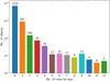 |
Fig. 1. Distribution of candidates by expert vote count during the first stage of the visual inspection. The bar heights represent the number of candidates that received the corresponding number of votes from the 12 experts. |
During the subsequent analysis, 32 of these 183 candidates were identified as duplicates, however, which were removed from the sample. These duplicates arose because the VIS source catalogue itself contains multiple entries for the same physical source, with slight positional shifts within 1′′ between the duplicate entries. This left 151 unique candidates, which then underwent a second, more rigorous round of visual inspection. Three visual inspectors completed only the first stage of inspection, while for the second stage, six new inspectors were added and worked alongside nine inspectors who had completed both stages, bringing the total to 15 experts. These experts graded each candidate based on the presence of lensing features. They used a grading scheme (see AB24) that categorised the candidates into four grades: A, B, C, and X. In short, the grading scheme implies the following:
-
Grade A represents definite lenses with clear lensing features.
-
Grade B suggests the presence of lensing features, but a confirmation requires additional data.
-
Grade C indicates lensing features that might also be attributed to other physical phenomena.
-
Grade X refers to objects that are definitively not lenses.
4. Results
We present an overview of the grade A, B, and C candidates found in our search of the ERO fields. Our search method combined multiple CNN models with visual classification to ensure a robust candidate identification.
4.1. CNNs with visual classification
We identified a total of 97 lens candidates, distributed as 14 grade A candidates, 31 grade B candidates, 52 grade C candidates, and 54 objects as grade X (non-lenses) during our visual inspection process. The catalogue of all these candidates is shown in Table C.1.
The 14 grade A candidates that represent definite lenses are shown in Fig. 2. The 31 grade B candidates, which exhibit strong lensing features but require further confirmation, are represented by 12 examples in Fig. 3. Because there are so many grade C candidates, we show 12 representative examples in Fig. 4 of the 52 grade C objects that show potential lensing characteristics, but necessitate additional investigation. Complete mosaics of all candidates are provided in Appendix D.
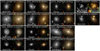 |
Fig. 2. Mosaic of the grade A lens candidates from the second round of visual inspection. For each candidate, we show the high-resolution IE-band cutout on the left and the lower-resolution HE, YE, IE composite on the right. The IAU name and field name are displayed at the top and bottom of the IE-band cutout, respectively, and the final joint grade is shown in red at the bottom of the composite cutout. Each cutout is 9 |


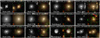 |
Fig. 3. Mosaic of the 12 out of 31 grade B lens candidates from the second round of visual inspection (see Appendix D for the complete sample). For each candidate, we show the high-resolution IE-band cutout on the left and the lower-resolution HE, YE, IE composite on the right. The IAU name and field name are displayed at the top and bottom of the IE-band cutout, respectively, and the final joint grade is shown in red at the bottom of the composite cutout. Each cutout is 9 |


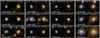 |
Fig. 4. Mosaic of the 12 out of 52 grade C lens candidates from the second round of visual inspection (see Appendix D for the complete sample). For each candidate, we show the high-resolution IE-band cutout on the left and the lower-resolution HE, YE, IE composite on the right. The IAU name and field name are displayed at the top and bottom of the IE-band cutout, respectively, and the final joint grade is shown in red at the bottom of the composite cutout. Each cutout is 9 |


4.2. CNN results
We illustrate the performance of each individual network in terms of the number of grade A, B and C candidates that were rejected across different grades in Table 1. We used the same respective thresholds for different CNNs as in PC24. We refer to this threshold as the reference threshold throughout this paper.
Number of candidates that was rejected by each CNN model at their respective reference thresholds for the different grades.
Table 1 demonstrates significant variations in the rejection rates among the models. Naberrie exhibits the highest rejection rate for grade A and B candidates. This suggests that its reference threshold value (pTHRESH = 0.9) may be too high for identifying prominent lensing candidates in these ERO fields. Conversely, Denselens demonstrates superior performance. It only fails to detect 1 out of 14 grade A candidates and 5 out of 31 grade B candidates. Lens-CLR and 4-Layer CNN follow closely, with very few rejections. While MRC-95 appears to have the second lowest rejection rate of total candidates among CNN models, Table 2 reveals that this apparent advantage is offset by a high number of FP. This diminishes its overall effectiveness.
Number of A, B, and C grade candidates passed by each CNN model at their respective reference thresholds at the expense of respective FP.
Table 2 demonstrates a clear distinction between the performance of the various CNN models in terms of grade A, B, and C candidate detection and FP. Denselens is the best-performing model with the lowest number of FP. Denselens, at a reference threshold of pontTHRESH = 0.23, detected 13 grade A, 26 grade B, and 36 grade C candidates while maintaining a relatively low number of FP of just 5265, suggesting it is effective at detecting lensing features without excessive FP. Lens-CLR, despite a higher FP count (27 026), still shows a strong performance. It passed a large number of grade A, B, and C candidates. In contrast, the other models struggled with precision, especially 4-Layer CNN and MRC-95, both of which produced an overwhelming number of FP, with MRC-95 producing 222 426 FP. This is a result of converting the multiple predictions for each object by the Mask R-CNN into a single prediction for the cutout.
4.3. Contamination rate
We evaluated the performance of the five models by comparing their contamination rates, defined as the ratio of FP to the total number of candidates classified as grades A, B, and C by each model, as shown in Fig. 5. Among the models, Denselens exhibits the best performance, achieving the lowest contamination rate of 70 at a reference threshold of pontTHRESH = 0.23. A contamination rate of 70 FP per TP is still too high for practical use in an automated pipeline, however, where CNNs would be employed without any human visual inspection. This contamination rate for the other ERO fields is significantly higher than the contamination rate for the Perseus field reported in PC24. This high false-positive rate may also be attributed to the selection of relatively simple constraints for creating cutouts for this 16 ERO fields (other than Perseus).
4.4. CNN performance
Figure 6 illustrates the relation between the total number of candidates and the contamination rate (FP/TP ratio) for various CNN models, including an ensemble of Denselens and Lens-CLR, where candidates were only classified as lenses when both models agreed above a common threshold (pTHRESH). Of all models, Denselens demonstrated a superior performance. It achieved a contamination rate lower than 100 for all threshold probabilities (pTHRESH) that exceeded 0.15. Lens-CLR exhibitsed satisfactory performance at pTHRESH = 0.95, where its contamination rate was also lower than 100. Given the strong individual performance of these two models, we propose to investigate an ensemble approach that combines Denselens and Lens-CLR to potentially further improve the classification accuracy and reduce contamination.
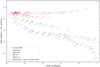 |
Fig. 6. Total number of candidates detected by individual CNN models and an ensemble CNN model (combining DenseLens and Lens-CLR) as a function of the contamination rate (FP/TP) at their respective thresholds. |
The ensemble model that combined Denselens and Lens-CLR demonstrated superior performance, as shown by the black dots in Fig. 6. This combined approach achieves the lowest contamination rate (FP/TP ratio), and it outperformed even the best individual Denselens model. In this ensemble model, a candidate is considered a true positive (TP) only if its classification prediction scores from both models exceed a common threshold pTHRESH. For instance, at pTHRESH = 0.50,
-
Denselens detected 43 candidates with ∼37 FP for each TP.
-
Lens-CLR identified 74 candidates, but with ∼407 FP per TP.
-
The ensemble model recovered 33 candidates with only 14 FP for each TP.
While it might be argued that the true-positive rate decreases along with the contamination rate, Fig. 6 illustrates that by selecting an appropriate pTHRESH value, the ensemble model consistently recovers the same number of candidates at a significantly lower contamination rate than any individual model. This improved performance stems from the diverse training datasets used for each model. The ensemble approach leverages the strengths of the two individual models, resulting in a more precise candidate selection while minimising FP. These findings suggest that an ensemble method might be a robust strategy for enhancing the overall performance of CNNs in detecting strong lensing candidates. Based on these results, we recommend implementing an ensemble approach of the best-performing CNNs for future Euclid automatic lens-detection pipelines.
Table 2 presents the reference threshold and the number of grade A, B, and C candidates recovered at that specific threshold. Fig. 6 indicates that the reference threshold that was determined using the Perseus field does not perform optimally when applied to other ERO fields, however. These CNN networks can achieve better contamination rates at thresholds different from the reference threshold.
Table 3 shows the grade A, B, and C candidate recovery at different thresholds for the Denselens and Lens-CLR models. This table demonstrates that we can recover candidates at a more acceptable contamination rate. For example, at pontTHRESH = 0.65, we recover 7 out of a total of 14 grade A candidates, 9 grade B candidates, and 8 grade C candidates at an acceptable contamination rate of 5 FP for every TP. At these acceptable contamination rates, a visual inspection can almost be completely eliminated. This paves the way for an automatic lens classification.
For the ensemble model of Denselens, and Lens-CLR, we show the detected pTHRESH, number of grade A, B, and C candidates, the total candidates, FP, the detected FP for every detected grade A candidate (FP/A), and the contamination rate (FP/TP).
In contrast, models such as 4-Layer CNN and MRC-95 show a significant rise in the contamination rate as the total number of detected grade A, B, and C candidates increases. This suggests that these models are more prone to FP, in particular, when they attempt to detect a larger number of candidates. Naberrie, in particular, shows the highest FP/TP ratio, and its performance worsens even when the pontTHRESH is increased to its reference pontTHRESH = 0.90. This suggests that the pontTHRESH value applied for the Perseus field is not optimal for all the other fields. Contamination rate of 4-Layer CNN, Naberrie and MRC-95 are never lower than 1000 on the ERO fields, regardless of any threshold (pontTHRESH). Naberrie was designed as a two-stage approach where the high scoring cutouts could be ruled out by inspecting the heat maps (Wilde 2023) produced by the model. This feature was not used to select the candidates in this paper, which explains the large number of FP.
4.5. Prediction
We compared our findings with the predictions made by Collett (2015), who estimated that the Euclid mission would discover approximately 170 000 strong gravitational lenses over its planned survey area of 15 000 square degrees. The 13 Euclid ERO fields we analysed cover a total area of 8.12 deg2, and we would therefore naively expect ∼90 strong lenses in the ERO area, although this is reduced to ∼70 when we applied our IE < 23 pre-selection. Our study identified 97 grade A, B, and C lens candidates. This number aligns closely with the theoretical expectations. Experience suggests, however, that most grade C candidates are unlikely to be lenses. Taking Collett (2015) as truth and pessimistically assuming that only our grade A candidates are lenses, we would conclude that our search is complete at ∼15% . If the grade B candidates were also all lenses, we would have found ∼60% of all the lenses with IE < 23 that are in the ERO fields. This incompleteness is expected for our conservative grading approach, which prioritised sample purity, and based on the limitations in our CNN training set diversity and the subjective nature of visual inspection. Future work will focus on improving the completeness through enhanced training sets, more sophisticated model architectures, and complementary detection techniques while maintaining a high sample purity.
5. Palomar spectroscopy
We obtained optical spectroscopic follow-up of several of the grade A and grade B candidates using the Double Spectrograph (DBSP; Oke & Gunn 1982) on the 5 m Hale telescope at Palomar Observatory between June and October 2024. Table 4 presents the targets for which we were able to measure at least one redshift in the candidate strong lens system. All the Palomar observing nights had seeing of ∼1 2. The June and July nights were photometric, while the October night had some clouds at the start and end of the night, but it was relatively clear at the time of the reported observation. For each observation, we obtained two or three exposures of 1200 s using the 1
 5 slit, the 600 lines blue grating (blazed at 4000 Å), the 5500 Å dichroic, and the 316 lines red grating (blazed at 7500 Å). The slits were aligned on the candidate lensing galaxy at a position angle to cover the putative lens feature. The data were reduced using standard techniques within the Image Reduction and Analysis Facility (IRAF).
Palomar spectroscopy of strong lens candidates.
All the lensing galaxies proved to be early-type galaxies with Ca H & K absorption and strong 4000 Å breaks. One grade A system, EUCL J081705.61+702348.8, revealed redshifts for the foreground lensing galaxy and the background source galaxy, where the latter had a slightly (∼1 7) offset emission line at 9222.8 Å (Fig. 7). If the emission feature were associated with the primary target galaxy at z = 0.335, the implied rest-frame wavelength would be 6908 Å, which does not correspond to any strong spectral features in galaxies, particularly early-type galaxies. Instead, the most plausible identification is [O II] emission from a lensed star-forming galaxy at z = 1.475.
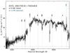 |
Fig. 7. Spectrum of the grade A strong lens candidate EUCL J081705.61+702348.8 obtained at Palomar Observatory. The spectrum reveals an early-type galaxy at z = 0.335 with several characteristic absorption lines in addition to a strong 4000 Å break. There is a strong additional line at 9222.8 Å that we associate with [O II] emission from the lensed source galaxy at z = 1.475. |
To further confirm the lensing nature of EUCL J081705.61+702348.8, we modelled the system using the Euclid strong lens modelling pipeline implemented in PyAutoLens (Nightingale et al. 2018, 2021). A full description of the pipeline and application to a larger sample of lenses will be provided in the Q1 data release papers (Euclid Collaboration 2025; Walmsley et al. 2025). Figure 8 presents the results for the VIS optical image. The foreground lens galaxy light was subtracted by fitting it with a multi-Gaussian expansion composed of 60 Gaussians (He et al. 2024). This revealed two distinct arcs in locations that are consistent with a singular isothermal ellipsoid (SIE) mass model configuration. PyAutoLens fitted the SIE lens model, which, as shown in the right panel of Fig. 8, accurately ray-traces the two arcs to the same region of the source plane. The source reconstruction revealed two separate doubly imaged emission components that lie outside the tangential caustic, but within the radial caustic. This is consistent with the tangential and radial critical curves predicted by our SIE mass model for this lens system. The SIE lens mass model includes an external shear, and the inferred Einstein radius is 1 18 ± 0
 03.
03.
 |
Fig. 8. Lens model of the grade A system EUCL J081705.61+702348.8, created using the Euclid strong lens modelling pipeline implemented with PyAutoLens (Nightingale et al. 2018, 2021). The panels show (i) the observed VIS optical image; (ii) the lens-subtracted image; (iii) the lens model reconstruction of the lensed source; and (iv) the source galaxy reconstructed unlensed emission in the source plane. The system is accurately modelled, providing strong evidence of its lensing nature. The mass model is a singular isothermal ellipsoid with external shear, the lens light is modelled using a multi-Gaussian expansion (He et al. 2024), and the source is reconstructed on an adaptive Delaunay mesh. The inferred Einstein radius is 1 |


6. Discussion and conclusions
We have presented a catalogue of strong gravitational lens candidates identified in the Euclid ERO that cover 13 fields with a total area of 8.12 deg2. Our search method combined multiple CNN models with visual classification and yielded 97 lens candidates: 14 grade A, 31 grade B, and 52 grade C candidates. This multi-stage approach that used CNNs for the initial candidate selection followed by visual inspection has proven effective in producing a high-purity sample, in particular, for grade A and B candidates.
Our analysis of five CNN models revealed significant variations in their performance characteristics. Denselens emerged as the best-performing individual model. It achieved the lowest contamination rate of 70 FP per TP at its reference threshold. This model successfully detected 13 out of 14 grade A candidates while maintaining relatively low false-positive rates. Lens-CLR also demonstrated a strong performance. It passed a large number of grade A, B, and C candidates, but with a higher false-positive count of 27 026 compared to the 5265 of Denselens. The remaining models, including Naberrie, 4-Layer,CNN, and MRC-95, exhibited substantially higher contamination rates, which makes them less suitable for an automated pipeline implementation without extensive visual inspection.
The ensemble approach combining Denselens and Lens-CLR represented a significant advancement in our method. It achieved contamination rates as low as five FP per TP at appropriately selected thresholds. At pTHRESH = 0.65, this ensemble model recovered seven grade A, nine grade B, and eight grade C candidates with acceptable contamination levels that would enable near-automated classification pipelines. This demonstrates that leveraging the complementary strengths of multiple CNN architectures trained on diverse datasets can substantially improve the candidate selection precision.
While spectroscopic follow-up of our highest-quality candidate EUCL J081705.61+702348.8 provided an initial validation of our classification, additional observations are needed to fully establish the robustness of our system. Our spectroscopic analysis revealed an emission line at 9222.8 Å that was most plausibly identified as [O II] from a lensed star-forming galaxy at z = 1.475, measuring the redshifts for the foreground lensing galaxy (z = 0.335) and the background source galaxy. The lens model implemented in PyAutoLens fitted the two distinct arcs and revealed a source reconstruction with two doubly imaged emission components located outside the tangential caustic but within the radial caustic. This confirmed the strong lensing configuration. The lens modelling measured an Einstein radius of 1 18 ± 0
 03.
03.
We compared our findings with theoretical predictions, which indicated that the discovery of 97 candidates (across all grades) in 8.12 deg2 is consistent with previous estimates of ∼70 strong lenses in this area (after applying our IE < 23 pre-selection). Taking a conservative approach where only grade A candidates are considered confirmed lenses, our search achieved a completeness of ∼15% that increased to ∼60% when grade B candidates were included. Our lower completeness rate compared to Zoobot1 (Walmsley et al. 2023), which identified 61 out of 68 known lenses (∼90% completeness) in RP24, may be attributed to the fact that the true number of lenses in our study is unknown. This makes it more challenging than studies where the ground truth was known. Furthermore, our selection of only the top 650 candidates based on the geometric mean scores for each field, while chosen to maintain a reasonable balance between completeness and false positive rate, may have excluded some genuine lens candidates that received lower CNN scores.
This work serves as a guide for future Euclid lens searches. It demonstrates that a broad initial CNN search followed by visual inspection is essential for building high-purity lens samples. While our method established the foundational approach for the lens identification in Euclid ERO data, operational implementation across the full 15 000 deg2 survey will require ensemble-learning methods and active learning frameworks that iteratively retrain models on visually validated samples to substantially reduce the number of candidates requiring human inspection while achieving higher completeness. The full potential of the Euclid lens searches will be realised through a multi-band analysis, expanded spectroscopic follow-up campaigns, and advanced automated selection techniques like this. The lens-modelling pipeline we demonstrated here for EUCL J081705.61+702348.8 provides a template for future systematic analyses of larger lens samples in upcoming Euclid data releases.
Acknowledgments
B.C.N. acknowledges support of DSSC and HPC cluster of RUG. J. A. A. B. and B. C. acknowledge support from the Swiss National Science Foundation (SNSF). C.T acknowledges the INAF grant 2022 LEMON. A.M.G. acknowledges the support of project PID2022-141915NB-C22 funded by MCIU/AEI/10.13039/501100011033 and FEDER/UE. Based on observations obtained at the Hale Telescope, Palomar Observatory, as part of a collaborative agreement between the Caltech Optical Observatories and the Jet Propulsion Laboratory. This work made use of Astropy: a community-developed core Python package and an ecosystem of tools and resources for astronomy (Astropy Collaboration 2013, 2018, 2022), NumPy (Harris et al. 2020), Matplotlib (Hunter 2007), and pandas (McKinney 2011). This work has made use of the Early Release Observations (ERO) data from the Euclid/ mission of the European Space Agency (ESA), 2024, https://doi.org/10.57780/esa-qmocze3. The Euclid Consortium acknowledges the European Space Agency and a number of agencies and institutes that have supported the development of Euclid, in particular the Agenzia Spaziale Italiana, the Austrian Forschungsförderungsgesellschaft funded through BMK, the Belgian Science Policy, the Canadian Euclid Consortium, the Deutsches Zentrum für Luft- und Raumfahrt, the DTU Space and the Niels Bohr Institute in Denmark, the French Centre National d’Etudes Spatiales, the Fundação para a Ciência e a Tecnologia, the Hungarian Academy of Sciences, the Ministerio de Ciencia, Innovación y Universidades, the National Aeronautics and Space Administration, the National Astronomical Observatory of Japan, the Nederlandse Onderzoekschool Voor Astronomie, the Norwegian Space Agency, the Research Council of Finland, the Romanian Space Agency, the State Secretariat for Education, Research, and Innovation (SERI) at the Swiss Space Office (SSO), and the United Kingdom Space Agency. A complete and detailed list is available on the Euclid web site (https://www.euclid-ec.org).
References
- Andika, I. T., Suyu, S. H., Cañameras, R., et al. 2023, A&A, 678, A103 [NASA ADS] [CrossRef] [EDP Sciences] [Google Scholar]
- Astropy Collaboration (Robitaille, T. P., et al.) 2013, A&A, 558, A33 [NASA ADS] [CrossRef] [EDP Sciences] [Google Scholar]
- Astropy Collaboration (Price-Whelan, A. M., et al.) 2018, AJ, 156, 123 [Google Scholar]
- Astropy Collaboration (Price-Whelan, A. M., et al.) 2022, ApJ, 935, 167 [NASA ADS] [CrossRef] [Google Scholar]
- Atek, H., Gavazzi, R., Weaver, J., et al. 2025, A&A, 697, A15 [NASA ADS] [CrossRef] [EDP Sciences] [Google Scholar]
- Barnabè, M., Spiniello, C., Koopmans, L. V. E., et al. 2013, MNRAS, 436, 253 [Google Scholar]
- Barroso, J. A., O’riordan, C., Clément, B., et al. 2025, A&A, 697, A14 [Google Scholar]
- Biesiada, M. 2006, Phys. Rev. D, 73, 023006 [Google Scholar]
- Birrer, S., & Amara, A. 2018, Phys. Dark Universe, 22, 189 [NASA ADS] [CrossRef] [Google Scholar]
- Birrer, S., Millon, M., Sluse, D., et al. 2024, Space Sci. Rev., 220, 48 [NASA ADS] [CrossRef] [Google Scholar]
- Broadhurst, T. J., Taylor, A. N., & Peacock, J. A. 1995, ApJ, 438, 49 [Google Scholar]
- Cañameras, R., Schuldt, S., Suyu, S., et al. 2020, A&A, 644, A163 [NASA ADS] [CrossRef] [EDP Sciences] [Google Scholar]
- Christ, C., Nord, B., Gozman, K., & Ottenbreit, K. 2020, AAS, 235, 303 [Google Scholar]
- Collett, T. E. 2015, ApJ, 811, 20 [NASA ADS] [CrossRef] [Google Scholar]
- Cropper, M., Pottinger, S., Niemi, S., et al. 2016, in SPIE 2016: Optical, Infrared, and Millimeter Wave (SPIE), 9904, 269 [Google Scholar]
- Cuillandre, J.-C., Bertin, E., Bolzonella, M., et al. 2025a, A&A, 697, A6 [Google Scholar]
- Cuillandre, J.-C., Bolzonella, M., Boselli, A., et al. 2025b, A&A, 697, A11 [Google Scholar]
- Davies, A., Serjeant, S., & Bromley, J. M. 2019, MNRAS, 487, 5263 [NASA ADS] [CrossRef] [Google Scholar]
- de Jong, J. T., Verdoes Kleijn, G. A., Kuijken, K. H., et al. 2013, Exp. Astron., 35, 25 [NASA ADS] [CrossRef] [Google Scholar]
- Despali, G., Vegetti, S., White, S. D. M., Giocoli, C., & van den Bosch, F. C. 2018, MNRAS, 475, 5424 [NASA ADS] [CrossRef] [Google Scholar]
- Euclid Collaboration (Scaramella, R., et al.) 2022, A&A, 662, A112 [NASA ADS] [CrossRef] [EDP Sciences] [Google Scholar]
- Euclid Collaboration (Cropper, M., et al.) 2025, A&A, 697, A2 [Google Scholar]
- Euclid Collaboration (Jahnke, K., et al.) 2025, A&A, 697, A3 [Google Scholar]
- Euclid Collaboration (Mellier, Y., et al.) 2025, A&A, 697, A1 [Google Scholar]
- Euclid Collaboration (Rojas, K., et al.) 2025, A&A, in press, https://doi.org/10.1051/0004-6361/202554605 [Google Scholar]
- Euclid Early Release Observations 2024, https://doi.org/10.57780/esa-qmocze3 [Google Scholar]
- Gavazzi, R., Treu, T., Koopmans, L. V. E., et al. 2008, ApJ, 677, 1046 [NASA ADS] [CrossRef] [Google Scholar]
- Gavazzi, R., Treu, T., Rhodes, J. D., et al. 2007, ApJ, 667, 176 [Google Scholar]
- Gentile, F., Tortora, C., Covone, G., et al. 2021, MNRAS, 510, 500 [NASA ADS] [CrossRef] [Google Scholar]
- Gilman, D., Du, X., Benson, A., et al. 2019, MNRAS, 492, L12 [Google Scholar]
- Grillo, C., Rosati, P., Suyu, S. H., et al. 2018, ApJ, 860, 94 [Google Scholar]
- Harris, C. R., Millman, K. J., van der Walt, S. J., et al. 2020, Nature, 585, 357 [NASA ADS] [CrossRef] [Google Scholar]
- He, K., Gkioxari, G., Dollár, P., & Girshick, R. 2017, in Proceedings of the IEEE International Conference on Computer Vision, 2961 [Google Scholar]
- He, Q., Li, H., Li, R., et al. 2020, MNRAS, 496, 4717 [Google Scholar]
- He, Q., Nightingale, J. W., Amvrosiadis, A., et al. 2024, MNRAS, 532, 2441 [Google Scholar]
- Hezaveh, Y. D., Dalal, N., Marrone, D. P., et al. 2016, ApJ, 823, 37 [Google Scholar]
- Hunt, L., Annibali, F., Cuillandre, J.-C., et al. 2025, A&A, 697, A9 [NASA ADS] [CrossRef] [EDP Sciences] [Google Scholar]
- Hunter, J. D. 2007, CiSE, 9, 90 [Google Scholar]
- Jacobs, C., Glazebrook, K., Collett, T., More, A., & McCarthy, C. 2017, MNRAS, 471, 167 [Google Scholar]
- Jacobs, C., Collett, T., Glazebrook, K., et al. 2019, MNRAS, 484, 5330 [NASA ADS] [CrossRef] [Google Scholar]
- Kingma, D. P., & Ba, J. 2015, in 3rd ICLR 2015, San Diego, CA, USA, May 7–9, 2015, Conference Track Proceedings, eds. Y. Bengio, & Y. LeCun [Google Scholar]
- Kluge, M., Hatch, N., Montes, M., et al. 2025, A&A, 697, A13 [NASA ADS] [CrossRef] [EDP Sciences] [Google Scholar]
- Kochanek, C. S., & Schechter, P. L. 2003, COAS, 2, 211 [Google Scholar]
- Koonce, B. 2021, in Convolutional Neural Networks with Swift for Tensorflow: Image Recognition and Dataset Categorization (Springer), 63 [Google Scholar]
- Koopmans, L. V. E. 2004, arXiv e-prints [arXiv:astro-ph/0412596] [Google Scholar]
- Koopmans, L. V. E., Bolton, A., Treu, T., et al. 2009, ApJ, 703, L51 [NASA ADS] [CrossRef] [Google Scholar]
- Lanusse, F., Ma, Q., Li, N., et al. 2018, MNRAS, 473, 3895 [Google Scholar]
- Leier, D., Ferreras, I., Saha, P., et al. 2016, MNRAS, 459, 3677 [NASA ADS] [CrossRef] [Google Scholar]
- Li, R., Frenk, C. S., Cole, S., et al. 2016, MNRAS, 460, 363 [NASA ADS] [CrossRef] [Google Scholar]
- Li, R., Frenk, C. S., Cole, S., Wang, Q., & Gao, L. 2017, MNRAS, 468, 1426 [NASA ADS] [CrossRef] [Google Scholar]
- Li, R., Shu, Y., & Wang, J. 2018, MNRAS, 480, 431 [NASA ADS] [CrossRef] [Google Scholar]
- Li, R., Napolitano, N. R., Tortora, C., et al. 2020, ApJ, 899, 30 [Google Scholar]
- Li, R., Napolitano, N., Spiniello, C., et al. 2021, ApJ, 923, 16 [NASA ADS] [CrossRef] [Google Scholar]
- Limousin, M., Kneib, J.-P., & Natarajan, P. 2005, MNRAS, 356, 309 [Google Scholar]
- Lintott, C. J., Schawinski, K., Slosar, A., et al. 2008, MNRAS, 389, 1179 [NASA ADS] [CrossRef] [Google Scholar]
- Manjón-García, A. 2021, Ph.D. Thesis, University of Cantabria, Spain [Google Scholar]
- Marleau, F., Cuillandre, J.-C., Cantiello, M., et al. 2025, A&A, 697, A12 [NASA ADS] [CrossRef] [EDP Sciences] [Google Scholar]
- Marshall, P. J., Hogg, D. W., Moustakas, L. A., et al. 2009, ApJ, 694, L924 [Google Scholar]
- Martín, E., Žerjal, M., Bouy, H., et al. 2025, A&A, 697, A7 [NASA ADS] [CrossRef] [EDP Sciences] [Google Scholar]
- Massari, D., Dalessandro, E., Erkal, D., et al. 2025, A&A, 697, A8 [Google Scholar]
- McKinney, W., et al. 2011, PyHPC, 14, 1 [Google Scholar]
- Meneghetti, M., Bartelmann, M., Dolag, K., et al. 2005, A&A, 442, 413 [NASA ADS] [CrossRef] [EDP Sciences] [Google Scholar]
- Metcalf, R. B., Meneghetti, M., Avestruz, C., et al. 2019, A&A, 625, A119 [NASA ADS] [CrossRef] [EDP Sciences] [Google Scholar]
- Nadler, E. O., Birrer, S., Gilman, D., et al. 2021, ApJ, 917, 7 [NASA ADS] [CrossRef] [Google Scholar]
- Nagam, B. C., Koopmans, L. V. E., Valentijn, E. A., et al. 2023, MNRAS, 523, 4188 [NASA ADS] [CrossRef] [Google Scholar]
- Nagam, B. C., Koopmans, L. V. E., Valentijn, E. A., et al. 2024, MNRAS, 533, 1426 [Google Scholar]
- Nightingale, J. W., Dye, S., & Massey, R. J. 2018, MNRAS, 478, 4738 [Google Scholar]
- Nightingale, J. W., Massey, R. J., Harvey, D. R., et al. 2019, MNRAS, 489, 2049 [NASA ADS] [Google Scholar]
- Nightingale, J., Hayes, R., Kelly, A., et al. 2021, J. Open Source Softw., 6, 2825 [NASA ADS] [CrossRef] [Google Scholar]
- Oguri, M., Inada, N., Strauss, M. A., et al. 2008, AJ, 135, 512 [NASA ADS] [CrossRef] [Google Scholar]
- Oke, J., & Gunn, J. 1982, PASP, 94, 586 [Google Scholar]
- O’Riordan, C. M., Despali, G., Vegetti, S., Lovell, M. R., & Moliné, Á. 2023, MNRAS, 521, 2342 [CrossRef] [Google Scholar]
- Pearce-Casey, R., Nagam, B. C., Clement, B., & Tortora, C. 2025, A&A, 696, A214 [NASA ADS] [CrossRef] [EDP Sciences] [Google Scholar]
- Petrillo, C. E., Tortora, C., Chatterjee, S., et al. 2017, MNRAS, 472, 1129 [Google Scholar]
- Petrillo, C. E., Tortora, C., Chatterjee, S., et al. 2019a, MNRAS, 482, 807 [NASA ADS] [Google Scholar]
- Petrillo, C. E., Tortora, C., Vernardos, G., et al. 2019b, MNRAS, 484, 3879 [Google Scholar]
- Pourrahmani, M., Nayyeri, H., & Cooray, A. 2018, ApJ, 856, 68 [NASA ADS] [CrossRef] [Google Scholar]
- Rezaei, S., McKean, J. P., Biehl, M., de Roo, W., & Lafontaine, A. 2022, MNRAS, 517, 1156 [NASA ADS] [CrossRef] [Google Scholar]
- Rhee, G. 1991, Nature, 350, 211 [Google Scholar]
- Rojas, K., Savary, E., Clément, B., et al. 2022, A&A, 668, A73 [NASA ADS] [CrossRef] [EDP Sciences] [Google Scholar]
- Ronneberger, O., Fischer, P., & Brox, T. 2015, in MICCAI (Springer), 234 [Google Scholar]
- Saifollahi, T., Voggel, K., Lançon, A., et al. 2025, A&A, 697, A10 [NASA ADS] [CrossRef] [EDP Sciences] [Google Scholar]
- Sarbu, N., Rusin, D., & Ma, C.-P. 2001, ApJ, 561, L147 [Google Scholar]
- Savary, E., Rojas, K., Maus, M., et al. 2022, A&A, 666, A1 [NASA ADS] [CrossRef] [EDP Sciences] [Google Scholar]
- Schaefer, C., Geiger, M., Kuntzer, T., & Kneib, J.-P. 2018, A&A, 611, A2 [NASA ADS] [CrossRef] [EDP Sciences] [Google Scholar]
- Şengül, A. Ç., & Dvorkin, C. 2022, MNRAS, 516, 336 [CrossRef] [Google Scholar]
- Sereno, M. 2002, A&A, 393, 757 [NASA ADS] [CrossRef] [EDP Sciences] [Google Scholar]
- Shajib, A. J., Mozumdar, P., Chen, G. C.-F., et al. 2023, A&A, 673, A9 [NASA ADS] [CrossRef] [EDP Sciences] [Google Scholar]
- Shiralilou, B., Martinelli, M., Papadomanolakis, G., et al. 2020, JCAP, 04, 057 [Google Scholar]
- Shlivko, D., & Steinhardt, P. J. 2024, Phys. Lett. B, 855, 138826 [Google Scholar]
- Spiniello, C., Barnabè, M., Koopmans, L. V. E., & Trager, S. C. 2015, MNRAS, 452, L21 [Google Scholar]
- Stern, D., Jimenez, R., Verde, L., Kamionkowski, M., & Stanford, S. A. 2010, JCAP, 02, 008 [CrossRef] [Google Scholar]
- Tan, M., & Le, Q. 2021, in Proceedings of the 38th International Conference on Machine Learning, eds. M. Meila, & T. Zhang (PMLR), PMLR, 139, 10096 [Google Scholar]
- Tortora, C., Napolitano, N. R., Romanowsky, A. J., & Jetzer, P. 2010, ApJ, 721, L1 [NASA ADS] [CrossRef] [Google Scholar]
- Treu, T., & Koopmans, L. V. E. 2002, ApJ, 575, 87 [NASA ADS] [CrossRef] [Google Scholar]
- Treu, T., Auger, M. W., Koopmans, L. V. E., et al. 2010, ApJ, 709, 1195 [Google Scholar]
- Treu, T., Suyu, S. H., & Marshall, P. J. 2022, A&AR, 30, 8 [Google Scholar]
- Turyshev, S. G., & Toth, V. T. 2022, MNRAS, 513, 5355 [Google Scholar]
- van den Oord, A., Li, Y., & Vinyals, O. 2018, arXiv e-prints [arXiv:1807.03748] [Google Scholar]
- Vegetti, S., & Vogelsberger, M. 2014, MNRAS, 442, 3598 [NASA ADS] [CrossRef] [Google Scholar]
- Vegetti, S., Birrer, S., Despali, G., et al. 2024, Space Sci. Rev., 220, 58 [CrossRef] [Google Scholar]
- Walmsley, M., Allen, C., Aussel, B., et al. 2023, J. Open Source Softw., 8, 5312 [NASA ADS] [CrossRef] [Google Scholar]
- Walmsley, M., Holloway, P., Lines, N., et al. 2025, A&A, submitted [arXiv:2503.15324] [Google Scholar]
- Weaver, J., Taamoli, S., McPartland, C., et al. 2025, A&A, 697, A16 [NASA ADS] [CrossRef] [EDP Sciences] [Google Scholar]
- Wilde, J. W. 2023, Ph.D. Thesis, The Open University [Google Scholar]
- Wilde, J., Serjeant, S., Bromley, J. M., et al. 2022, MNRAS, 512, 3464 [Google Scholar]
- Zhang, T.-J. 2004, ApJ, 602, L5 [Google Scholar]
- Zitrin, A., Rosati, P., Nonino, M., et al. 2012, ApJ, 749, 97 [NASA ADS] [CrossRef] [Google Scholar]
Appendix A: Summary of the ERO fields
We present here the summary of the 16 Euclid ERO fields (except Perseus). The Euclid VIS instrument provides high-quality optical imaging through a single broad optical band (550-900 nm). The VIS camera features a pixel scale of 0 1 per pixel. The point spread function (PSF) of VIS has a full width at half maximum (FWHM) of ≲ 0
 18 across the entire field of view (Cropper et al. 2016). For the ERO fields, each pointing consists of four dithered exposures of 565 seconds each, resulting in a total exposure time of 2260 seconds. This yields a typical 5σ point-source depth of IE ≈26.2 mag (Euclid Collaboration: Scaramella et al. 2022). The VIS images demonstrate excellent depth and resolution, with a median signal-to-noise ratio (S/N) of ∼10σ for objects at IE = 24.5 mag.
Summary of all the 16 Euclid ERO Fields (except Perseus) including their corresponding area, and their corresponding catalogue size, which represents the number of sources in each field.
Appendix B: CNN score statistics across fields
We provide summary statistics of the CNN scores across all surveyed fields. Table B.1 presents the mean and standard deviation of the top-650 scoring candidates for each field, calculated separately for each individual CNN model.
Summary of mean and standard deviation of CNN scores for the top-650 candidates in each field for each individual CNN model.
Appendix C: Lens candidates
We show the details of 97 lens candidates which are distributed as 14 grade A candidates, 31 grade B candidates, and 52 grade C candidates. We have checked our Grade A and Grade B candidates against the strong lensing database (SLED; https://sled.amnh.org/) and confirmed that none of them were previously known.
Probable lens candidates discovered with CNN classifiers. ID, IAU Name, Fields, RA, DEC, Classification prediction scores for five different networks (P1, P2, P3, P4 and P5), Geometric Mean (GM) of the five prediction scores and visual inspection grade are shown. Here, P1 refers to the Lens-CLR network, P2 refers to the Denselens, P3 refers to the 4-Layer CNN, P4 refers to the Naberrie and P5 refers to the MRC95.
Appendix D: Full Mosaics
This appendix presents the complete mosaics of all grade B and grade C candidates from the second round of visual inspection. Representative subsets of these figures are shown in the main text (Fig. 3 and Fig. 4).
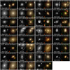 |
Fig. D.1. Mosaic of the grade B lens candidates from the second round of visual inspection. For each candidate, we show the high-resolution IE-band cutout on the left and the lower-resolution HE, YE, IE composite on the right. The IAU name and field name are displayed at the top and bottom of the IE-band cutout, respectively, and the final joint grade is shown in red at the bottom of the composite cutout. Each cutout is 9 |


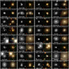 |
Fig. D.2. Mosaic of the 32 out of 52 grade C lens candidates from the second round of visual inspection. For each candidate, we show the high-resolution IE-band cutout on the left and the lower-resolution HE, YE, IE composite on the right. The IAU name and field name are displayed at the top and bottom of the IE-band cutout, respectively, and the final joint grade is shown in red at the bottom of the composite cutout. Each cutout is 9 |


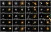 |
Fig. D.3. Mosaic of the remaining 20 grade C lens candidates from the second round of visual inspection. For each candidate, we show the high-resolution IE-band cutout on the left and the lower-resolution HE, YE, IE composite on the right. The IAU name and field name are displayed at the top and bottom of the IE-band cutout, respectively, and the final joint grade is shown in red at the bottom of the composite cutout. Each cutout is 9 |


All Tables
Number of candidates that was rejected by each CNN model at their respective reference thresholds for the different grades.
Number of A, B, and C grade candidates passed by each CNN model at their respective reference thresholds at the expense of respective FP.
For the ensemble model of Denselens, and Lens-CLR, we show the detected pTHRESH, number of grade A, B, and C candidates, the total candidates, FP, the detected FP for every detected grade A candidate (FP/A), and the contamination rate (FP/TP).
Summary of all the 16 Euclid ERO Fields (except Perseus) including their corresponding area, and their corresponding catalogue size, which represents the number of sources in each field.
Summary of mean and standard deviation of CNN scores for the top-650 candidates in each field for each individual CNN model.
Probable lens candidates discovered with CNN classifiers. ID, IAU Name, Fields, RA, DEC, Classification prediction scores for five different networks (P1, P2, P3, P4 and P5), Geometric Mean (GM) of the five prediction scores and visual inspection grade are shown. Here, P1 refers to the Lens-CLR network, P2 refers to the Denselens, P3 refers to the 4-Layer CNN, P4 refers to the Naberrie and P5 refers to the MRC95.
All Figures
|
Fig. 1. Distribution of candidates by expert vote count during the first stage of the visual inspection. The bar heights represent the number of candidates that received the corresponding number of votes from the 12 experts. |
| In the text | |
|
Fig. 2. Mosaic of the grade A lens candidates from the second round of visual inspection. For each candidate, we show the high-resolution IE-band cutout on the left and the lower-resolution HE, YE, IE composite on the right. The IAU name and field name are displayed at the top and bottom of the IE-band cutout, respectively, and the final joint grade is shown in red at the bottom of the composite cutout. Each cutout is 9 |
| In the text | |
|
Fig. 3. Mosaic of the 12 out of 31 grade B lens candidates from the second round of visual inspection (see Appendix D for the complete sample). For each candidate, we show the high-resolution IE-band cutout on the left and the lower-resolution HE, YE, IE composite on the right. The IAU name and field name are displayed at the top and bottom of the IE-band cutout, respectively, and the final joint grade is shown in red at the bottom of the composite cutout. Each cutout is 9 |
| In the text | |
|
Fig. 4. Mosaic of the 12 out of 52 grade C lens candidates from the second round of visual inspection (see Appendix D for the complete sample). For each candidate, we show the high-resolution IE-band cutout on the left and the lower-resolution HE, YE, IE composite on the right. The IAU name and field name are displayed at the top and bottom of the IE-band cutout, respectively, and the final joint grade is shown in red at the bottom of the composite cutout. Each cutout is 9 |
| In the text | |
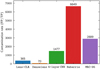 |
Fig. 5. Contamination rate of each CNN model at their respective thresholds in Table 2. |
| In the text | |
|
Fig. 6. Total number of candidates detected by individual CNN models and an ensemble CNN model (combining DenseLens and Lens-CLR) as a function of the contamination rate (FP/TP) at their respective thresholds. |
| In the text | |
|
Fig. 7. Spectrum of the grade A strong lens candidate EUCL J081705.61+702348.8 obtained at Palomar Observatory. The spectrum reveals an early-type galaxy at z = 0.335 with several characteristic absorption lines in addition to a strong 4000 Å break. There is a strong additional line at 9222.8 Å that we associate with [O II] emission from the lensed source galaxy at z = 1.475. |
| In the text | |
|
Fig. 8. Lens model of the grade A system EUCL J081705.61+702348.8, created using the Euclid strong lens modelling pipeline implemented with PyAutoLens (Nightingale et al. 2018, 2021). The panels show (i) the observed VIS optical image; (ii) the lens-subtracted image; (iii) the lens model reconstruction of the lensed source; and (iv) the source galaxy reconstructed unlensed emission in the source plane. The system is accurately modelled, providing strong evidence of its lensing nature. The mass model is a singular isothermal ellipsoid with external shear, the lens light is modelled using a multi-Gaussian expansion (He et al. 2024), and the source is reconstructed on an adaptive Delaunay mesh. The inferred Einstein radius is 1 |
| In the text | |
|
Fig. D.1. Mosaic of the grade B lens candidates from the second round of visual inspection. For each candidate, we show the high-resolution IE-band cutout on the left and the lower-resolution HE, YE, IE composite on the right. The IAU name and field name are displayed at the top and bottom of the IE-band cutout, respectively, and the final joint grade is shown in red at the bottom of the composite cutout. Each cutout is 9 |
| In the text | |
|
Fig. D.2. Mosaic of the 32 out of 52 grade C lens candidates from the second round of visual inspection. For each candidate, we show the high-resolution IE-band cutout on the left and the lower-resolution HE, YE, IE composite on the right. The IAU name and field name are displayed at the top and bottom of the IE-band cutout, respectively, and the final joint grade is shown in red at the bottom of the composite cutout. Each cutout is 9 |
| In the text | |
|
Fig. D.3. Mosaic of the remaining 20 grade C lens candidates from the second round of visual inspection. For each candidate, we show the high-resolution IE-band cutout on the left and the lower-resolution HE, YE, IE composite on the right. The IAU name and field name are displayed at the top and bottom of the IE-band cutout, respectively, and the final joint grade is shown in red at the bottom of the composite cutout. Each cutout is 9 |
| In the text | |
Current usage metrics show cumulative count of Article Views (full-text article views including HTML views, PDF and ePub downloads, according to the available data) and Abstracts Views on Vision4Press platform.
Data correspond to usage on the plateform after 2015. The current usage metrics is available 48-96 hours after online publication and is updated daily on week days.
Initial download of the metrics may take a while.