| Issue |
A&A
Volume 702, October 2025
|
|
|---|---|---|
| Article Number | A47 | |
| Number of page(s) | 11 | |
| Section | Stellar structure and evolution | |
| DOI | https://doi.org/10.1051/0004-6361/202554429 | |
| Published online | 06 October 2025 | |
ASASSN-13dn: A luminous and double-peaked type II supernova
1
Instituto de Estudios Astrofísicos, Facultad de Ingeniería y Ciencias, Universidad Diego Portales, Avenida Ejercito Libertador 441, Santiago, Chile
2
Millennium Institute of Astrophysics MAS, Nuncio Monseñor Sotero Sanz 100, Off. 104, Providencia, Santiago, Chile
3
Carnegie Observatories, Las Campanas Observatory, Casilla 601, La Serena, Chile
4
Instituto de Astrofísica de La Plata (IALP), CCT-CONICET-UNLP., Paseo del Bosque S/N, B1900FWA La Plata, Argentina
5
Facultad de Ciencias Astronomicas y Geofisicas, Universidad Nacional de La Plata, Instituto de Astrofisica de La Plata (IALP), CONICET, Paseo del Bosque SN, B1900FWA La Plata, Argentina
6
Kavli Institute for the Physics and Mathematics of the Universe (WPI), The University of Tokyo, 5-1-5 Kashiwanoha, Kashiwa, Chiba, 277-8583, Japan
7
National Astronomical Observatory of Japan, National Institutes of Natural Sciences, 2-21-1 Osawa, Mitaka, Tokyo, 181-8588, Japan
8
Graduate Institute for Advanced Studies, SOKENDAI, 2-21-1 Osawa, Mitaka, Tokyo, 181-8588, Japan
9
School of Physics and Astronomy, Monash University, Clayton, Victoria, 3800, Australia
10
Department of Astronomy, The Ohio State University, 140 W 18th Avenue, Columbus, OH, 43210, USA
11
Center for Cosmology and AstroParticle Physics, 191 W Woodruff Avenue, Columbus, OH, 43210, USA
12
Institute for Astronomy, University of Hawaii, 2680 Woodlawn Drive, Honolulu, HI, 96822, USA
⋆ Corresponding author: This email address is being protected from spambots. You need JavaScript enabled to view it.
Received:
8
March
2025
Accepted:
18
July
2025
Abstract
Aim. We present observations of ASASSN-13dn, one of the first supernovae discovered by ASAS-SN and a new member of the rare group of known type II luminous supernovae (LSNe). It was discovered near maximum light, reaching an absolute magnitude of Mv ∼ −19 mag, placing this object between normal luminosity type II supernovae and superluminous supernovae.
Methods. We performed a detailed analysis of the photometric and spectroscopic data of ASASSN-13dn. The spectra are characterized by broad lines, in particular the Hα lines, where we measure expansion velocities ranging between 14 000 and 6000 km s−1 over the first 100 days. Hα dominates the nebular spectra, and we detect a narrow P-Cygni absorption within the broader emission line with an expansion velocity of 1100 km s−1. Photometrically, its light curve shows a re-brightening of ∼0.6 mag in the gri bands starting 25 ± 2 days after discovery, with a secondary peak at ∼73d followed by an abrupt and nearly linear decay of 0.09 mag d−1 for the next 35 days. At later times, after a drop of 4 magnitudes from the second maximum, the light curves of ASASSN-13dn show softer undulations from 125 to 175 days.
Results. We compared ASASSN-13dn with other type II LSNe in the literature, finding no match to either the light curve or spectroscopic properties. We discuss the main powering mechanism and suggest that interaction between the ejecta and a dense circumstellar material produced by eruptions from a luminous blue variable-like progenitor could potentially explain the observations.
Key words: supernovae: general / supernovae: individual: ASASSN-13dn
© The Authors 2025
 Open Access article, published by EDP Sciences, under the terms of the Creative Commons Attribution License (https://creativecommons.org/licenses/by/4.0), which permits unrestricted use, distribution, and reproduction in any medium, provided the original work is properly cited.
This article is published in open access under the Subscribe to Open model. This email address is being protected from spambots. You need JavaScript enabled to view it. to support open access publication.
1. Introduction
Core-collapse supernovae (CCSNe) are the explosive ends of massive stars (MZAMS > 8 M⊙; Filippenko 1997; Heger et al. 2003). When the progenitor star retains its hydrogen envelope, the spectra are dominated by prominent Balmer lines from hydrogen. These hydrogen-rich supernovae (SNe) are classified as type II SNe. Based on their photometric properties, type II SNe are usually classified into two major sub-classes: type II-P and II-L (Barbon et al. 1979). If the light curve is characterized by a plateau of nearly constant luminosity after the peak, it is classified as type II-P. On the other hand, light curves characterized by a linear decay after their peak luminosity are classified as type II-L. Nonetheless, recent studies have shown that a continuous distribution better describes the wide variety of light curve shapes (Anderson et al. 2014).
The spectroscopic properties of type II SNe define two additional sub-classes: type IIb and type IIn. Type IIb SNe are stripped-envelope supernovae (SESNe) that retain a fraction of their hydrogen envelopes at the time of the explosion (Filippenko et al. 1993). They exhibit strong hydrogen and helium lines in early phases, while hydrogen lines disappear and helium lines dominate in later stages. Type IIn SNe are characterized by persistent narrow emission lines with velocities of < 1000 km/s; these narrow lines are produced by photoionized and unshocked circumstellar material (CSM; Schlegel 1990). The narrow lines are frequently found on top of a broad spectral feature, which is produced by the shocked ejecta and CSM. The SN emission is dominated by the interaction between the SN ejecta and the dense CSM.
The main powering mechanisms for regular type II SNe are the energy of the explosion deposited in the envelope during shock wave propagation and the decay of the radioactive elements, mainly 56Ni, generated during explosive nucleosynthesis (Branch & Wheeler 2017). After the photospheric phase, when the energy deposited in the envelope is released via recombination processes, the tail of the light curve is mainly powered by the energy deposition from the radioactive decay of 56Ni →56Co →56Fe. With full γ-ray trapping, the expected decline rate during this phase is 0.98 mag per 100 days (Woosley et al. 1989; Nadyozhin 1994).
In the last two decades, a new class of transient phenomena has been identified. While regular CCSNe have an absolute magnitude range of MV ∼ −14 to −18.5 (Li et al. 2011), explosions with peak absolute magnitudes brighter than MV ≤ −21 mag had been classified as superluminous SNe (SLSNe; Quimby et al. 2011). However, this luminosity threshold is not definitive; De Cia et al. (2018) show that SLSNe are a distinct spectroscopic sub-class that sometimes overlaps in luminosity with the normal population of SESNe.
Over the last few years, the luminosity gap between regular CCSNe and SLSNe has been gradually populated by theso-called luminous supernovae (LSNe). With peak absolute magnitudes MV < ∼ − 19, these objects appear to spectroscopically bridge the gap between regular CCSNe and SLSNe, suggesting a continuum in their spectroscopic properties (Gomez et al. 2022; Nicholl 2021). While the discovery of type II SNe within this luminosity range dates back several decades (e.g. SN 1979C, Branch et al. 1981; SN 1998S, Liu et al. 2000; SN2003bg, Hamuy et al. 2009), it was not until Pessi et al. (2023) that these kinds of explosions were formally recognized as a subgroup of type II SNe. Their study found that this subgroup evolves more slowly than typical type II SNe, exhibiting broader emission lines and ejecta velocities of around v ∼ 10 000 km s−1.
The light curves of CCSNe are generally characterized by a single peak. However, recent studies have increasingly identified double or multi-peaked light curves, particularly among SESNe (Gutiérrez et al. 2021; Chen et al. 2023; Cartier et al. 2024). These findings challenge traditional models and require the consideration of alternative powering mechanisms to account for the observations. Among the proposed central engine power sources are newly formed magnetars undergoing spin-down (Kasen & Bildsten 2010; Woosley 2010) and fallback accretion onto a stellar-mass black hole (Dexter & Kasen 2013). These mechanisms have been invoked to explain the extreme luminosities (Moriya et al. 2018), long-duration light curves (Arcavi et al. 2017), and distinct spectroscopic features observed in individual SNe (e.g. Nicholl et al. 2018). Additionally, the hypothesis of a double nickel distribution in SESNe has provided an explanation for the observed light curves (Orellana & Bersten 2022).
Due to the limited number of well-characterized multi-peaked type II SNe, there is insufficient consensus regarding the mechanisms responsible for their powering. The observed properties, particularly the high luminosities, are difficult to reconcile with the typical powering mechanisms, suggesting that additional mechanisms are at play (Orellana et al. 2018).
An example of this debate surrounds iPTF14hls (Arcavi et al. 2017), a type II SN with long, luminous, and multi-peaked light curves whose spectra show no clear signatures of ejecta-CSM interaction. No narrow emission lines were observed in this event, and an equal increase in luminosity at all wavelengths ruled out the ejecta-CSM interaction scenario. Fallback into a stellar-mass black hole was adopted as the leading powering mechanism to explain the bumpy light curve (Arcavi et al. 2017). Dessart (2018) argue in favour of a magnetar-powered model to explain the observed properties of this SN. A type II LSN with a similar discussion is ASASSN-15nx (Bose et al. 2018). The linearity of its light curve might indicate that it is powered purely by radioactive decay with a significant gamma-ray leakage factor, but the 56Ni mass necessary to explain the peak luminosity is too high for CCSNe (Müller et al. 2017). Chugai (2019) discusses the possibility of this SN being powered by a magnetar after modelling the light curve and the [O I] 6300, 6364 Å doublet in late-time spectra.
Typically, a standard type II SN is understood as the explosive endpoint of a red supergiant, and many of its observed characteristics align with this scenario. However, Morozova et al. (2017) and Dessart & Hillier (2022) argue that the continuum observed in the light curve properties could be attributed to variations in CSM properties. In some cases, observed features such as the interaction of ejecta with fast-moving pre-explosion eruptions challenge the standard red supergiant scenario and suggest alternative progenitor types, including luminous blue variable (LBV)-like stars. This is exemplified by events such as SN 2009ip, a type IIn SN, where pre-explosion eruptions and their interaction with the surrounding CSM indicate an LBV-like progenitor (Mauerhan et al. 2013).
In this paper, we report on the unique luminous type II SN ASASSN-13dn. With a peak absolute magnitude of MV ∼ −19 mag, the SN shows a secondary maximum 73 days after maximum light; At 125 days, the SN has dropped 4 magnitudes from the secondary maximum and begins to show bumps. Spectroscopically, ASASSN-13dn displays broad hydrogen emission lines with ejecta velocities of ∼14 000 km s−1. In Sect. 2 we present the data collected, describe the reduction process, and briefly describe the host galaxy properties. In Sect. 3 we describe both the photometry and spectroscopic data of ASASSN-13dn. Then, in Sect. 4 we discuss possible power sources and the ejecta-CSM interaction signatures found in the observations. Finally, in Sect. 5 we present our conclusions.
2. Data
2.1. Discovery and host galaxy
ASASSN-13dn was discovered by the All-Sky Automated Survey for Supernovae (ASAS-SN; Shappee et al. 2014; Kochanek et al. 2017) on December 5, 2013, 04:09 UT at a V-band magnitude of 15.70 by Shappee et al. (2013) and on December 17, 2013, at 21:03 UT the SN was classified as a type II SN (Martini et al. 2013). It exploded in the outer regions of the star-forming galaxy SDSS J125258.03+322444.3 (z = 0.022636) at  ,
,  (J2000.0). We adopted the Virgo infall only distance reported on NASA/IPAC Extragalactic Database of 96.0 Mpc (μ = 34.91 ± 0.15 mag) using a flat cosmology with H0 = 73 km s−1 Mpc −1 and Ωm = 0.27. At this distance, the SN is ∼11.8 kpc from the centre of its host galaxy (see Fig. 1). We neglected any host-galaxy extinction due to the absence of any Na I D absorption in all our spectra, which indicates a very low or negligible contribution from the host. Therefore, we adopted a total reddening of E(B − V)=0.014 mag (Schlafly & Finkbeiner 2011), assuming a RV = 3.1 (Cardelli et al. 1989), which results in AV = 0.043 mag.
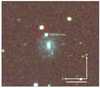 |
Fig. 1. LCOGTN gri composite image of ASASSN-13dn. |
Taggart & Perley (2021) includes this galaxy in their photometric analysis of CCSNe hosts and estimates a total stellar mass of log10(M⋆/M⊙) = 9.85 ± 0.05 and a specific star-formation rate (sSFR) of log10(sSFR/yr−1) =  . We extracted a spectrum of the host galaxy with the Multi-Object Double Spectrograph (MODS) at the Large Binocular Telescope (LBT) on July 2, 2015, when the SN had already faded. From the spectrum, we detect nebular emission lines of Hα, Hβ, [O III] 5007 Å, and [N II] 6583 Å. We used the scaling relation of Kennicutt (1998) to estimate a star-formation rate (SFR) of the host from the Hα luminosity of log10(SFR) = 0.79 M⊙ yr−1. Using emission line ratios and the scaling relations presented in Marino et al. (2013), we estimate an oxygen abundance of 12+log(O/H) = 8.33 and 12+log(O/H) = 8.38 with the O3N2 and N2 methods, respectively. These values are consistent with 12+log(O/H) = 8.39 and 12+log(O/H) = 8.34 for the O3N2 and N2 indicators, the mean values of the oxygen abundances of the sample of CCSNe from Pessi et al. (2023).
2.2. Photometry
The ASAS-SN V-band photometry using image subtraction is reported in Table A.1. The SN was followed up with the Liverpool Telescope (LT; Steele et al. 2004) 2.0m and the Las Cumbres Observatory Global Telescope Network (LCOGTN; Brown et al. 2013) 1.0m telescopes from discovery until ∼180 days after the first detection. The griz photometry was obtained performing point-spread-function photometry with DoPhot (Schechter et al. 1993; Alonso-García et al. 2012), using photometry of stars in the field from SDSS DR12 (Alam et al. 2015) to perform photometric calibrations. Image subtraction was performed on the g and r bands using a single archival SDSS DR12 image as a template. No major differences with the non-subtracted photometry were seen, so no further attempts were made to improve the photometry.
The SN exploded during a seasonal gap, and no rise to peak was seen in the light curve. The last non-detection was on July 24.25, 2013, 134d before the discovery (Martini et al. 2013), so the explosion date is poorly constrained. In the first 10 days, the V-band light curve slowly faded and then transitioned to a steeper decay rate. This suggests that the SN was discovered shortly after maximum light. For simplicity, we assumed that the first detection is close enough to the epoch of maximum light, and all reported times are relative to the discovery.
2.3. Spectroscopy
We obtained 13 optical spectra between +9d and +176d after maximum light using the Kitt Peak Ohio State Multi-Object Spectrograph (KOSMOS; Martini et al. 2014) on the KPNO Mayall 4m telescope, the Multi-Object Double Spectrograph (MODS; Pogge et al. 2010) on the LBT (Hill et al. 2010), and the Dual Imaging Spectrograph (DIS) on the Apache Point Observatory (APO) 3.5m telescope. The spectra were reduced using standard techniques in IRAF that included basic 2D image reductions (overscan and bias subtraction, flat-fielding), extraction of 1D spectra, wavelength calibration using HeNeAr lamps, and flux calibration using a standard star observed on the night of the observation. We corrected the absolute flux calibration of the spectra by matching synthetic photometry from the spectra to the photometric light curve in the r band.
3. Analysis
3.1. Light curve
ASASSN-13dn was discovered at an absolute magnitude of MV = −18.94 ± 0.21 mag. We fitted a second-order polynomial to the V-band photometry, calculated the mean-fit polynomial derivative, and found that this value is constantly decreasing. As the first detection is the point where the derivative is close to zero, we assumed that the maximum light is at MJD = 56631.2 ± 1.2. Using the r band as a reference, we defined four different sections of the light curve: (1) An initial decline from first detection to +48d; (2) A rise from +49d to a secondary peak at +73d. For the following days, it slowly decays to: (3) A second and steeper decline from +91d to +132d, and (4) A bumpy tail from +132d to the end of the observations. Fitting a quadratic polynomial to the gri bands between +32d and +62d, we find a minimum at +48.2 ± 0.8 days (MJD = 56681.05). The light curve has a nearly linear decay of 4.4 mag/100d with a statistical error of 0.1 mag after the first 10 days. We observe that the SN reaches the secondary peak at different epochs for the individual gri bands. Specifically, the later the peak occurs, the bluer the corresponding band (see Table A.2).
The light curve brightens ∼0.6 mag from +48d to +73d and becomes bluer, reaching its bluest colour near the secondary peak. Next, the light curve decays 0.6 mag in ∼15 days. This peak is followed by a faster decay of 9.3 mag/100d with a statistical error of 0.1 mag for the next 35 days. There is a second minimum at +132d and wiggles in the light curve can be observed. Figure 2 shows the light curve of ASASSN-13dn, where the described phases can be clearly distinguished.
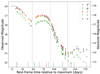 |
Fig. 2. ASASSN-13dn light curve. A secondary peak is observed ∼73 days after the first detection. In the tail of the light curve, clear signs of ejecta-CSM interaction are seen in the wiggles. The decline in slope after the secondary peak is faster than the decline after the first peak. The lines at the bottom mark the epochs where spectroscopic data are available. The vertical lines divide the light curve into the phases described in Sect. 3.1. |
The luminosity of this object places it into the group of hydrogen-rich luminous SNe. In Fig. 4 we present a comparison between ASASSN-13dn r-band light curve with SN 1987A and type II LSNe from the literature. Immediately after maximum, most of the SNe in Fig. 4 show a similar decay rate until ∼45d, with the extreme exception of the fast-declining SN 2017hxz. After this phase, the variety of light curves makes them difficult to compare; nonetheless, linear decay at different phases is the common behaviour, and the secondary peak of ASASSN-13dn is unique among this group. After this, ASASSN-13dn’s decay is faster than the other SNe presented here at similar phases. This is particularly clear when comparing the r-band light curve of ASASSN-13dn with ASASSN-15nx (Bose et al. 2018), an almost perfectly linearly declining type II SN.
Even though the light curves presented in Fig. 4 show a wide variety in their behaviour, the g − r colours (corrected for Galactic extinction) shown in Fig. 3 are remarkably consistent between type II LSNe. A slight change towards the blue between +65d and +125d is detected, but it is still consistent with the blue colours of type II LSNe. This change occurs at the same epochs where the secondary peak occurs.
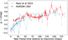 |
Fig. 3. g − r colour evolution of ASASSN-13dn compared with the type II LSNe presented in Pessi et al. (2023). Despite the variety of light curve shapes, the colours are consistent between objects. |
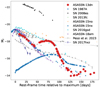 |
Fig. 4. Comparison of the r-band absolute magnitude evolution with other type II LSNe and SN 1987A. The phase is with respect to the maximum brightness. The bumps of ASASSN-13dn are not seen in other objects. The adopted maximum light date in MJD, distance (Mpc), and AV for each SN are, respectively: SN 1987A1: 49849.8, 0.05, 0.206 (Hamuy & Suntzeff 1990); SN 2008es: 54599.3, 1013.2, 0.032 (Miller et al. 2009) SN 2013fc: 56530.8, 83.2, 2.914 (Kangas et al. 2016); ASASSN-15no: 57235.5, 153.5, 0.045 (Benetti et al. 2018); ASASSN-15nx: 57219.1, 127.25, 0.22 (Bose et al. 2018) SN 2016gsd: 57662.5, 311.6, 0.254 (Reynolds et al. 2020); ASASSN-18am: 58142.6, 140.5, 0.027 (Bose et al. 2021); SN 2017cfo: 57838.0, 178.2, 0.066; SN 2017hbj: 58031.0, 75.0, 0.095; SN 2017hxz: 58070.0, 330.6, 0.128; SN 2018aql: 58206.0, 321.4, 0.052; and SN 2018eph: 58342.0, 121.8, 0.066 (Pessi et al. 2023). For SN1987A and SN2008es we used the R-band photometry. Note that the phase reported for SN 1987A is relative to the explosion and not the maximum. |
3.2. Bolometric light curve
We estimated the bolometric and pseudo-bolometric evolution using superbol.py (Nicholl 2018) to fit a modified blackbody to the photometry. The bolometric light curve integrates the model between 1500 and 25 000 Å while the pseudo-bolometric light curve only uses the wavelength range of the observed griz photometry. Since it is the best sampled photometric band, we used the r-band detections as the reference light curve. The z band was extrapolated assuming a constant z − r colour from peak to first z-detection at +65d. The resulting bolometric light curve, effective temperature, and blackbody radius are presented in Fig. 5. We estimate a maximum bolometric luminosity of 1.3 ± 0.6 × 1043 erg s−1 and a total radiated energy of Etot > 4.5 × 1049 erg.
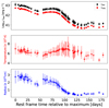 |
Fig. 5. Bolometric light curve and best-fit parameters from the blackbody fitting for ASASSN-13dn. Upper panel: Bolometric and pseudo-bolometric light curves. Middle and bottom panels: Effective temperature and blackbody radius derived from superbol.py, respectively. The increase at +40d might indicate an outward movement of the photosphere. |
An abrupt increase of 1015 cm in the radius at +55 days is observed, and at the same time, a slow rise in the temperature of 2 × 10³ K occurred. Simultaneously, the observed colours in Fig. 3 became bluer, consistent with the increasing temperature at the same epochs. This suggests an outward movement of the photosphere, potentially driven by an additional energy source boosting the light curves at this time.
The wiggles at the end of the light curve are not consistent with a radioactive decay-powered explosion. Therefore, we can only place an upper limit on the 56Ni synthesized in the explosion. Assuming a rise time between 15 and 25 days and, considering that the luminosity at +132d of 1.45 × 1041 erg s−1 is nickel-powered with full trapping of gamma-rays, we used Nadyozhin (1994) to estimate an upper limit of ∼0.02 M⊙ of 56Ni, which is a factor of two lower than the mean nickel mass for the type II SNe of M(56Ni) = 0.046 M⊙ (Müller et al. 2017) and M(56Ni) = 0.036 M⊙ reported by Martinez et al. (2022).
3.3. Spectra
Between +9d and +176d, 13 optical spectra of ASASSN-13dn were taken. The spectra are characterized by a broad Hα emission line with velocities measured from the full width at half maximum (FWHM) higher than 10 000 km s−1 until 86d post-maximum. Broad Fe II at λ4924 Å and λ5018 Å lines are detected, but during the evolution of ASASSN-13dn those lines are blended with the Hβ emission line and themselves, so no further analysis was done with the Fe II features. Na I at λ5889.9 Å and the Ca triplet at λ8498 Å, λ8542 Å, and λ8662 Å are also detected. Davis et al. (2019) published a near-infrared spectrum of ASASSN-13dn at +77d (MJD = 56711) that is mainly dominated by hydrogen, showing strong Pγ at λ1.094 μm, Pβ at λ1.282 μm, and Pα at λ1.875 μm. The spectroscopic evolution of ASASSN-13dn is presented in Fig. 6, and the spectroscopic log is in Table A.3.
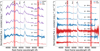 |
Fig. 6. Spectroscopic evolution of ASASSN-13dn. The flux has been normalized to the maximum of Hα for visibility purposes. |
In Fig. 7 we compare the spectra from +9d to +38d with other early spectra of type II LSNe. ASASSN-13dn shows a strong emission line of Hα with a weak P-Cygni absorption, blended Fe II lines, and a weak Na I emission profile. The broad hydrogen profile at this phase is only comparable with the type IIb SN 2003bg Hamuy et al. (2009). Before +30d, SN 2016gsd (Reynolds et al. 2020), SN 2017hbj (Pessi et al. 2023), SN 2017hxz (Pessi et al. 2023), and SN 2018eph (Pessi et al. 2023) are mainly a blue featureless continuum.
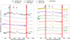 |
Fig. 7. Comparison of ASASSN-13dn spectra with those of type II LSNe studied in literature at different epochs. Left: ASASSN-13dn peak spectra with SN 2003bg (Hamuy et al. 2009), ASASSN-15nx (Bose et al. 2018), and SN 2016gsd (Reynolds et al. 2020). Spectra of SN 2017hxz, SN 2017hbj, and SN 2018eph are from Pessi et al. (2023). Right: Comparison of ASASSN-13dn secondary peak spectra with those of ASASSN-15nx (Bose et al. 2018) and SN 2016gsd (Reynolds et al. 2020). Spectra of SN 2017hxz, SN 2017hbj, and SN 2018eph are from Pessi et al. (2023). Phases reported in this figure are relative to the maximum luminosity reported in the references. |
Between +50d and +100d, all the spectra in Fig. 7 are characterized by strong and broad Balmer emission lines. Boxy Hα emission profiles are seen in the spectra of SN 2018eph and SN 2017hbj. A strong Ca II triplet at λ8498 Å, λ8542 Å and λ8662 Å is also present in SN 2017hbj and ASASSN-15nx (Bose et al. 2018). Both ASASSN-13dn and SN 2017hxz show an asymmetry towards the red wing of the Hα line, which is not seen in other SNe. With the exception of SN 2016gsd Reynolds et al. (2020), P-Cygni absorption at these phases is either weak or not detected.
At later epochs, the spectra are dominated by Balmer emission lines with profiles that deviate from a single Gaussian component. Although the spectra of the other type II LSNe shown in Fig. 8 are characterized by a broad and boxy Hα emission line, the spectra of ASASSN-13dn are dominated by a narrow Hα profile, with an absorption within the emission line at λ6540 Å. He I at λ7065 Å, λ7281 Å and Ca IIλ8498 Å, λ8542 Å, and λ8662 Å lines are observed in nebular spectra of ASASSN-15nx and SN 2016gsd. Helium is not detected in ASASSN-13dn, and a weak calcium line is detected in the last spectrum (ϕ + 176d).
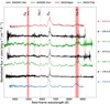 |
Fig. 8. Comparison of ASASSN-13dn late spectra with those of ASASSN-15nx (Bose et al. 2018), SN 2016gsd (Reynolds et al. 2020), and SN 2017hbj (Pessi et al. 2023). The reported phases are relative to the maximum luminosity reported in the references. |
3.4. Hα evolution
The Hα line profile and evolution shown in Fig. 9 is complex. In the first two spectra, at +9d and +11d, the Hα peak is blueshifted by 2174 km s−1. From +38d to +86d, a shoulder appears on the red wing of the emission line. In the +98d spectra, the line shows bumps towards the red and the blue sections of the emission line, and finally, the blue bump seen at +98d evolves into a narrow P-Cygni profile detected between +135d and +147d.
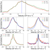 |
Fig. 9. Hα evolution of ASASSN-13dn. Top: Spectra close to the first detection, broad Hα lines with velocities (vFWHM) close to 14 000 km s−1, and a blueshifted peak. Middle: Persistent asymmetries towards the red part of the line from +38d to +98d at ∼5000 km s−1. Bottom: Last epochs of the light curve. Hα shows asymmetries and a strong P-Cygni profile at +140d. This absorption has a velocity of ∼1100 km s−1. |
The blueshifted peak of the emission observed in the +9d and +11d spectra has a velocity of 2174 km s−1 and is consistent with that observed by Pessi et al. (2023) at later epochs for other type II LSNe, nonetheless, it is not detected in the observations at +38d after peak. During the following observations, from +38d to +86d, a small but persistent shoulder appears on the red wing of Hα at 6678 Å. It is detected in every spectrum between +38d and +98d; it is most prominent at +82d, which coincides with the secondary peak in the light curve. A similar structure is present in the Hβ line profile, particularly clear at +52d and +82d. Figure 10 shows the emission profiles of Hα and Hβ at +82d where the shoulder is observed in bothprofiles with similar velocities, indicating that this structure is most likely related to asymmetries in the ejecta rather than the He II line.
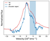 |
Fig. 10. Hα and Hβ emission lines from the +82d spectrum. The blue region marks the shoulder detected in both Hα and Hβ. The flux was normalized to the peak of the emission for visibility purposes. |
We calculated the FWHM velocity (vFWHM) and the velocity of the P-Cygni absorption trough (vPcyg) from the Hα line in ASASSN-13dn. To fit and subtract the pseudo-continuum of the line, we used PYTHON’s package specutils (Earl et al. 2022) in the range of the line profile for each spectrum. We also calculated the pseudo-equivalent width (pEW) of the line. This parameter quantifies the strength of the line compared to a pseudo-continuum, arbitrarily defined. In this case, we used the same specutils package to redefine a pseudo-continuum in the range of the Hα emission. For both vFWHM and pEW, we determined the uncertainties by randomly varying the wavelength range used to determine the pseudo-continuum by ±5 Å in a normal distribution. The evolution of the vFWHM and vPcyg velocities are presented in Fig. 11.
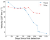 |
Fig. 11. Velocity evolution of ASASSN-13dn. The vFWHM corresponds to the velocity measured from the FWHM of the Hα emission, and the vPcyg is the velocity measured from the P-Cygni trough. |
In Fig. 12 we show the Hα velocity measured from the FWHM (vFWHM) and pEW evolution of ASASSN-13dn compared with the samples of normal type II SNe from Gutiérrez et al. (2017) and type II LSNe from Pessi et al. (2023). The velocity and pEW evolution of ASASSN-13dn is consistent with type II LSNe. Between +9d and +98d, the P-Cygni velocities are always higher than 10 000 km s−1, but at +140d and +176d spectra, the absorption was not detected. The Hα profile evolution is presented in Fig. 9. In the last three spectra, a P-Cygni profile inside the hydrogen line at λ6550 Å is detected, and a velocity of 1100 km s−1 was measured.
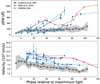 |
Fig. 12. Hα FWHM velocities (vFWHM) and pEW of ASASSN-13dn compared with the sample of type II LSNe from Pessi et al. (2023) and the type II SN sample from Gutiérrez et al. (2017). |
4. Discussion
In this section we explore different scenarios that could explain the luminosity and light curve features of ASASSN-13dn. Although the power source remains unclear, several signs of ejecta-CSM interaction are seen in the observations. The presence of a weak P-Cygni profile in the Hα line has been interpreted as a consequence of interaction in type II SNe (Gutiérrez et al. 2014).
A shoulder at ∼4100 km s−1, detected in both the Hα and Hβ profiles near the second peak, is consistent with this interaction. Observed between +38d and +86d, it matches the rest wavelength of He I emission, but it is most likely related to the ejecta-CSM interaction as it is also detected in the Hβ line at a similar velocity (see Fig. 10). A similar feature is described by Dessart & Hillier (2022) in models and is associated with an increase in the interaction power of the model.
In the later phases, the double-peaked Hα profile and the bumpy light curve – particularly the wiggles observed after +128d – indicate a continued interaction between the ejecta and the surrounding material. The P-Cygni absorption profiles at +140d, +147d, and +176d, with a velocity of 1100 km s−1, suggest interaction with a stellar wind or eruption from a massive progenitor star (Smith 2014). Similar profiles were observed in SN 2009ip, a type IIn SN, by Mauerhan et al. (2013), who proposed an LBV-like progenitor to explain the high velocity of the CSM shell. A comparable light curve signature, including similar wiggles, was observed in the type IIn SN iPTF13z, where the authors suggested that the interaction between the ejecta and denser CSM regions produced by LBV-like progenitor eruptions was responsible (Nyholm et al. 2017).
In this scenario, three dense CSM shells at distances of ∼4.9 × 1015 cm, ∼1.3 × 1016 cm, and ∼1.6 × 1016 cm, can produce the interaction signs at the secondary peak and subsequent wiggles observed in the light curve. The peak at +73d arises from the initial collision between the SN ejecta and the innermost CSM shell. The wiggles in the light curve result from continued interaction with the more distant shells.
These distances were determined by interpolating the Hα FWHM velocity (vFWHM; Fig. 11) and integrating the interpolated velocities to calculate the distance travelled by the material at specific epochs. Assuming a rise time of 20 days and a constant velocity of 12 000 km s−1 up to day +9d, the secondary peak at +73d and the wiggles at +138d and +170d align with these shell locations. Assuming a velocity of the progenitor eruption/wind between 100 and 1000 km s−1, the first shell is inferred to have been ejected between 25 and 2.5 years, prior to the explosion while the later shells, based on a CSM velocity of 1100 km s−1 measured from the +140d Hα spectrum 9 were produced 4.9 and 5.7 years before the explosion.
Using these observations, the properties of the CSM can be constrained. The wind-density parameter is defined by ̇M/ , where VCSM is the CSM velocity, VSN is the ejecta velocity, L the luminosity, and ̇M is the mass-loss rate. Using the bolometric luminosity of the first wiggle at +154d of 1.3 × 1043 erg s−1 and a mean velocity of 11 000 km s−1 from the P-Cygni absorption, we calculated a wind-density parameter of 1.7 × 10¹⁶ g cm−1. Additionally, with the CSM velocity measured at +140d, we estimate a mass-loss rate ̇M ∼ 0.08 M⊙ yr−1 in this scenario.
The light curve of ASASSN-13dn, shown in Fig. 2, displays notable features, including a secondary peak and bumps at later times. In Sect. 3.1 we measure the slopes of the light curve in different sections, finding a rapid decline immediately after the peak, followed by an even steeper decay after the secondary peak. The presence of CSM-ejecta interactions is known to enhance early-time luminosity, resulting in a rapidly declining light curve (Morozova et al. 2017). The irregularities, particularly the wiggles observed post +128d, coincide with the appearance of the P-Cygni absorption at 1100 km s−1 in the Hα emission, further reinforcing the signature of ejecta-CSM interaction.
Energy injection by the spin-down of a newly born magnetar (Kasen & Bildsten 2010; Woosley 2010) has been proposed to explain the extreme luminosities of transients, particularly H-poor SLSNe (Chatzopoulos et al. 2013; Nicholl et al. 2018; Hsu et al. 2021). This scenario has been proposed for a few hydrogen-rich SNe (iPTF14hls, Dessart 2018; OGLE-2014-SN-073, Dessart & Audit 2018; Orellana et al. 2018) as well as more normal SESNe (Rodríguez et al. 2024). In the case of ASASSN-13dn, a delayed power injection from a magnetar may boost the luminosity and explain the secondary peak.
Such power sources can increase the continuum emission without significantly affecting the spectral features, consistent with the relatively little spectral evolution observed during this phase. Likewise, interaction with a structured CSM–depending on its geometry–can enhance the luminosity without altering the spectral lines, as has been noted in other interacting transients.
The interaction between stars in a binary system has been proposed to explain pre-peak luminosity bumps, double-peaked light curves, and late-time wiggles (Dessart et al. 2024). A recent example of a SN with late-time wiggles is SN 2022jli, a type Ic SN whose light curve shows periodic undulations that might be explained by the stripping of the outer envelope of a companion star (Chen et al. 2024; Cartier et al. 2024). This is in good agreement with the periodic displacement of the peak emission lines on the same timescale. Although the stripping of the outer layers of a companion could form a complex CSM structure, which can explain the different structures in the emission lines of ASASSN-13dn, we cannot determine periodicity in the wiggles of the light curve.
A mixture of several power sources is also a feasible scenario. Zhu et al. (2024) propose a model in which a magnetar formed in the SN can evaporate the outer layers of a companion star. The heating of the outer envelope can produce post-peak bumps and broaden the emission lines by accelerating the SN ejecta. A similar scenario could explain the secondary peak, the wiggles, and the high ejecta velocities observed in ASASSN-13dn.
5. Summary and conclusions
ASASSN-13dn is a unique example of a double-peaked type II LSN. We present an analysis of this hydrogen-rich SN, whose light curve exhibits a primary peak at MV ∼ −19 mag, placing it within the category of LSNe. Approximately 45 days after reaching peak luminosity, the brightness of the SN increases by 0.6 mag over a period of 30 days, reaching a secondary peak at +73 days. Then, the light curve shows a decline at a rate of ∼4.4 mag per 100 days. Finally, two distinct wiggles are observed in all bands from +125 days until the last detection.
Although ASASSN-13dn falls into the broad-line type II LSN group, some of the spectroscopic and photometric features differ from the sample shown by Pessi et al. (2023). Most LSNe are characterized by a blue continuum at early epochs, whereas the peak spectra of ASASSN-13dn are dominated by strong hydrogen emission lines. This leads to a g − r colour at the peak luminosity of ASASSN-13dn that is 0.4 mag redder than the type II LSNe in the Pessi et al. (2023) sample. This might indicate a problem with the phases calculated under the assumption that the first detection is the peak luminosity. Spectroscopically, ASASSN-13dn shows broad hydrogen emission lines from peak to +86d with measured FWHM velocities higher than 7000 km s−1. The P-Cygni trough velocity remains fairly constant until +98d at ∼11 000 km s−1. Finally, the P-Cygni trough at 1100 km s−1 in the last three spectra seems to indicate that the ejecta is interacting with a fast-moving CSM, probably produced by eruptions of an LBV-like progenitor.
Data availability
The full versions of the photometry tables are available at the CDS via https://cdsarc.cds.unistra.fr/viz-bin/cat/J/A+A/702/A47
Acknowledgments
E.H. thanks Priscilla Pessi and Claudia Gutierrez for the data sent via private communication. E.H. was financially supported by Becas-ANID scholarship #21222163 and by ANID, Millennium Science Initiative, AIM23-0001. J.L.P acknowledges support from ANID, Millennium Science Initiative, AIM23-0001. R.C. acknowledges support from Gemini ANID ASTRO21-0036.
References
- Alam, S., Albareti, F. D., Allende Prieto, C., et al. 2015, ApJS, 219, 12 [Google Scholar]
- Alonso-García, J., Mateo, M., Sen, B., et al. 2012, AJ, 143, 70 [Google Scholar]
- Anderson, J. P., González-Gaitán, S., Hamuy, M., et al. 2014, ApJ, 786, 67 [Google Scholar]
- Arcavi, I., Howell, D. A., Kasen, D., et al. 2017, Nature, 551, 210 [Google Scholar]
- Barbon, R., Ciatti, F., & Rosino, L. 1979, A&A, 72, 287 [Google Scholar]
- Benetti, S., Zampieri, L., Pastorello, A., et al. 2018, MNRAS, 476, 261 [NASA ADS] [CrossRef] [Google Scholar]
- Bose, S., Dong, S., Kochanek, C. S., et al. 2018, ApJ, 862, 107 [NASA ADS] [CrossRef] [Google Scholar]
- Bose, S., Dong, S., Kochanek, C. S., et al. 2021, MNRAS, 503, 3472 [Google Scholar]
- Branch, D., & Wheeler, J. C. 2017, Supernova Explosions (Springer-Verlag GmbH Germany) [Google Scholar]
- Branch, D., Falk, S. W., McCall, M. L., et al. 1981, ApJ, 244, 780 [Google Scholar]
- Brown, T. M., Baliber, N., Bianco, F. B., et al. 2013, PASP, 125, 1031 [Google Scholar]
- Cardelli, J. A., Clayton, G. C., & Mathis, J. S. 1989, ApJ, 345, 245 [Google Scholar]
- Cartier, R., Contreras, C., Stritzinger, M., et al. 2024, A&A, submitted [arXiv:2410.21381] [Google Scholar]
- Chatzopoulos, E., Wheeler, J. C., Vinko, J., Horvath, Z. L., & Nagy, A. 2013, ApJ, 773, 76 [NASA ADS] [CrossRef] [Google Scholar]
- Chen, Z. H., Yan, L., Kangas, T., et al. 2023, ApJ, 943, 41 [NASA ADS] [CrossRef] [Google Scholar]
- Chen, P., Gal-Yam, A., Sollerman, J., et al. 2024, Nature, 625, 253 [NASA ADS] [CrossRef] [Google Scholar]
- Chugai, N. N. 2019, Astron. Lett., 45, 427 [Google Scholar]
- Davis, S., Hsiao, E. Y., Ashall, C., et al. 2019, ApJ, 887, 4 [NASA ADS] [CrossRef] [Google Scholar]
- De Cia, A., Gal-Yam, A., Rubin, A., et al. 2018, ApJ, 860, 100 [NASA ADS] [CrossRef] [Google Scholar]
- Dessart, L. 2018, A&A, 610, L10 [NASA ADS] [CrossRef] [EDP Sciences] [Google Scholar]
- Dessart, L., & Audit, E. 2018, A&A, 613, A5 [Google Scholar]
- Dessart, L., & Hillier, D. J. 2022, A&A, 660, L9 [NASA ADS] [CrossRef] [EDP Sciences] [Google Scholar]
- Dessart, L., Gutiérrez, C. P., Ercolino, A., Jin, H., & Langer, N. 2024, A&A, 685, A169 [NASA ADS] [CrossRef] [EDP Sciences] [Google Scholar]
- Dexter, J., & Kasen, D. 2013, ApJ, 772, 30 [NASA ADS] [CrossRef] [Google Scholar]
- Earl, N., Tollerud, E., O’Steen, R., et al. 2022, https://doi.org/10.5281/zenodo.7348235 [Google Scholar]
- Filippenko, A. V. 1997, ARA&A, 35, 309 [NASA ADS] [CrossRef] [Google Scholar]
- Filippenko, A. V., Matheson, T., & Ho, L. C. 1993, ApJ, 415, L103 [NASA ADS] [CrossRef] [Google Scholar]
- Gomez, S., Berger, E., Nicholl, M., Blanchard, P. K., & Hosseinzadeh, G. 2022, ApJ, 941, 107 [NASA ADS] [CrossRef] [Google Scholar]
- Gutiérrez, C. P., Anderson, J. P., Hamuy, M., et al. 2014, ApJ, 786, L15 [CrossRef] [Google Scholar]
- Gutiérrez, C. P., Anderson, J. P., Hamuy, M., et al. 2017, ApJ, 850, 89 [CrossRef] [Google Scholar]
- Gutiérrez, C. P., Bersten, M. C., Orellana, M., et al. 2021, MNRAS, 504, 4907 [CrossRef] [Google Scholar]
- Hamuy, M., & Suntzeff, N. B. 1990, AJ, 99, 1146 [NASA ADS] [CrossRef] [Google Scholar]
- Hamuy, M., Deng, J., Mazzali, P. A., et al. 2009, ApJ, 703, 1612 [NASA ADS] [CrossRef] [Google Scholar]
- Heger, A., Fryer, C. L., Woosley, S. E., Langer, N., & Hartmann, D. H. 2003, ApJ, 591, 288 [CrossRef] [Google Scholar]
- Hill, J. M., Green, R. F., Ashby, D. S., et al. 2010, in Ground-based and Airborne Telescopes III, eds. L. M. Stepp, R. Gilmozzi,&H. J. Hall, SPIE Conf. Ser., 7733, 77330C [Google Scholar]
- Hsu, B., Hosseinzadeh, G., & Berger, E. 2021, ApJ, 921, 180 [CrossRef] [Google Scholar]
- Kangas, T., Mattila, S., Kankare, E., et al. 2016, MNRAS, 456, 323 [NASA ADS] [CrossRef] [Google Scholar]
- Kasen, D., & Bildsten, L. 2010, ApJ, 717, 245 [NASA ADS] [CrossRef] [Google Scholar]
- Kennicutt, R. C., Jr 1998, ARA&A, 36, 189 [NASA ADS] [CrossRef] [Google Scholar]
- Kochanek, C. S., Shappee, B. J., Stanek, K. Z., et al. 2017, PASP, 129, 104502 [Google Scholar]
- Li, W., Leaman, J., Chornock, R., et al. 2011, MNRAS, 412, 1441 [NASA ADS] [CrossRef] [Google Scholar]
- Liu, Q. Z., Hu, J. Y., Hang, H. R., et al. 2000, A&AS, 144, 219 [NASA ADS] [CrossRef] [EDP Sciences] [Google Scholar]
- Marino, R. A., Rosales-Ortega, F. F., Sánchez, S. F., et al. 2013, A&A, 559, A114 [NASA ADS] [CrossRef] [EDP Sciences] [Google Scholar]
- Martinez, L., Bersten, M. C., Anderson, J. P., et al. 2022, A&A, 660, A41 [NASA ADS] [CrossRef] [EDP Sciences] [Google Scholar]
- Martini, P., Elias, J., Points, S., et al. 2013, ATel, 5667, 1 [Google Scholar]
- Martini, P., Elias, J., Points, S., et al. 2014, in Ground-based and Airborne Instrumentation for Astronomy V, eds. S. K. Ramsay, I. S. McLean,&H. Takami, SPIE Conf. Ser., 9147, 91470Z [Google Scholar]
- Mauerhan, J. C., Smith, N., Filippenko, A. V., et al. 2013, MNRAS, 430, 1801 [NASA ADS] [CrossRef] [Google Scholar]
- Miller, A. A., Chornock, R., Perley, D. A., et al. 2009, ApJ, 690, 1303 [NASA ADS] [CrossRef] [Google Scholar]
- Moriya, T. J., Terreran, G., & Blinnikov, S. I. 2018, MNRAS, 475, L11 [NASA ADS] [CrossRef] [Google Scholar]
- Morozova, V., Piro, A. L., & Valenti, S. 2017, ApJ, 838, 28 [NASA ADS] [CrossRef] [Google Scholar]
- Müller, T., Prieto, J. L., Pejcha, O., & Clocchiatti, A. 2017, ApJ, 841, 127 [Google Scholar]
- Nadyozhin, D. K. 1994, ApJS, 92, 527 [Google Scholar]
- Nicholl, M. 2018, Res. Notes Am. Astron. Soc., 2, 230 [NASA ADS] [Google Scholar]
- Nicholl, M. 2021, Astron. Geophys., 62, 5.34 [NASA ADS] [CrossRef] [Google Scholar]
- Nicholl, M., Blanchard, P. K., Berger, E., et al. 2018, ApJ, 866, L24 [NASA ADS] [CrossRef] [Google Scholar]
- Nyholm, A., Sollerman, J., Taddia, F., et al. 2017, A&A, 605, A6 [NASA ADS] [CrossRef] [EDP Sciences] [Google Scholar]
- Orellana, M., & Bersten, M. C. 2022, A&A, 667, A92 [NASA ADS] [CrossRef] [EDP Sciences] [Google Scholar]
- Orellana, M., Bersten, M. C., & Moriya, T. J. 2018, A&A, 619, A145 [NASA ADS] [CrossRef] [EDP Sciences] [Google Scholar]
- Pessi, P. J., Anderson, J. P., Folatelli, G., et al. 2023, MNRAS, 523, 5315 [NASA ADS] [CrossRef] [Google Scholar]
- Pessi, T. T., Prieto, J. L., Anderson, J. P., et al. 2023, A&A, 677, A28 [NASA ADS] [CrossRef] [EDP Sciences] [Google Scholar]
- Pogge, R. W., Atwood, B., Brewer, D. F., et al. 2010, in Ground-based and Airborne Instrumentation for Astronomy III, eds. I. S. McLean,&S. K. Ramsay, H. Takami, SPIE Conf. Ser., 7735, 77350A [NASA ADS] [Google Scholar]
- Quimby, R. M., Kulkarni, S. R., Kasliwal, M. M., et al. 2011, Nature, 474, 487 [NASA ADS] [CrossRef] [Google Scholar]
- Reynolds, T. M., Fraser, M., Mattila, S., et al. 2020, MNRAS, 493, 1761 [NASA ADS] [CrossRef] [Google Scholar]
- Rodríguez, Ó., Nakar, E., & Maoz, D. 2024, Nature, 628, 733 [Google Scholar]
- Schechter, P. L., Mateo, M., & Saha, A. 1993, PASP, 105, 1342 [Google Scholar]
- Schlafly, E. F., & Finkbeiner, D. P. 2011, ApJ, 737, 103 [Google Scholar]
- Schlegel, E. M. 1990, MNRAS, 244, 269 [NASA ADS] [Google Scholar]
- Shappee, B. J., Stanek, K. Z., Kochanek, C. S., et al. 2013, ATel, 5665, 1 [Google Scholar]
- Shappee, B. J., Prieto, J. L., Grupe, D., et al. 2014, ApJ, 788, 48 [Google Scholar]
- Smith, N. 2014, ARA&A, 52, 487 [NASA ADS] [CrossRef] [Google Scholar]
- Steele, I. A., Smith, R. J., Rees, P. C., et al. 2004, in Ground-based Telescopes, eds. J. Oschmann,&M. Jacobus, SPIE Conf. Ser., 5489, 679 [NASA ADS] [CrossRef] [Google Scholar]
- Taggart, K., & Perley, D. A. 2021, MNRAS, 503, 3931 [NASA ADS] [CrossRef] [Google Scholar]
- Woosley, S. E. 2010, ApJ, 719, L204 [NASA ADS] [CrossRef] [Google Scholar]
- Woosley, S. E., Pinto, P. A., & Hartmann, D. 1989, ApJ, 346, 395 [NASA ADS] [CrossRef] [Google Scholar]
- Zhu, J.-P., Liu, L.-D., Yu, Y.-W., et al. 2024, ApJ, 970, L42 [Google Scholar]
Appendix A: Tables
ASASSN-13dn V-band photometry.
ASASSN-13dn secondary peak epochs, phases, and magnitude for individual gri bands.
Log of spectroscopic observations.
ASASSN-13dn griz photometry from LT and the LCOGTN (extract).
All Tables
ASASSN-13dn secondary peak epochs, phases, and magnitude for individual gri bands.
All Figures
|
Fig. 1. LCOGTN gri composite image of ASASSN-13dn. |
| In the text | |
|
Fig. 2. ASASSN-13dn light curve. A secondary peak is observed ∼73 days after the first detection. In the tail of the light curve, clear signs of ejecta-CSM interaction are seen in the wiggles. The decline in slope after the secondary peak is faster than the decline after the first peak. The lines at the bottom mark the epochs where spectroscopic data are available. The vertical lines divide the light curve into the phases described in Sect. 3.1. |
| In the text | |
|
Fig. 3. g − r colour evolution of ASASSN-13dn compared with the type II LSNe presented in Pessi et al. (2023). Despite the variety of light curve shapes, the colours are consistent between objects. |
| In the text | |
|
Fig. 4. Comparison of the r-band absolute magnitude evolution with other type II LSNe and SN 1987A. The phase is with respect to the maximum brightness. The bumps of ASASSN-13dn are not seen in other objects. The adopted maximum light date in MJD, distance (Mpc), and AV for each SN are, respectively: SN 1987A1: 49849.8, 0.05, 0.206 (Hamuy & Suntzeff 1990); SN 2008es: 54599.3, 1013.2, 0.032 (Miller et al. 2009) SN 2013fc: 56530.8, 83.2, 2.914 (Kangas et al. 2016); ASASSN-15no: 57235.5, 153.5, 0.045 (Benetti et al. 2018); ASASSN-15nx: 57219.1, 127.25, 0.22 (Bose et al. 2018) SN 2016gsd: 57662.5, 311.6, 0.254 (Reynolds et al. 2020); ASASSN-18am: 58142.6, 140.5, 0.027 (Bose et al. 2021); SN 2017cfo: 57838.0, 178.2, 0.066; SN 2017hbj: 58031.0, 75.0, 0.095; SN 2017hxz: 58070.0, 330.6, 0.128; SN 2018aql: 58206.0, 321.4, 0.052; and SN 2018eph: 58342.0, 121.8, 0.066 (Pessi et al. 2023). For SN1987A and SN2008es we used the R-band photometry. Note that the phase reported for SN 1987A is relative to the explosion and not the maximum. |
| In the text | |
|
Fig. 5. Bolometric light curve and best-fit parameters from the blackbody fitting for ASASSN-13dn. Upper panel: Bolometric and pseudo-bolometric light curves. Middle and bottom panels: Effective temperature and blackbody radius derived from superbol.py, respectively. The increase at +40d might indicate an outward movement of the photosphere. |
| In the text | |
|
Fig. 6. Spectroscopic evolution of ASASSN-13dn. The flux has been normalized to the maximum of Hα for visibility purposes. |
| In the text | |
|
Fig. 7. Comparison of ASASSN-13dn spectra with those of type II LSNe studied in literature at different epochs. Left: ASASSN-13dn peak spectra with SN 2003bg (Hamuy et al. 2009), ASASSN-15nx (Bose et al. 2018), and SN 2016gsd (Reynolds et al. 2020). Spectra of SN 2017hxz, SN 2017hbj, and SN 2018eph are from Pessi et al. (2023). Right: Comparison of ASASSN-13dn secondary peak spectra with those of ASASSN-15nx (Bose et al. 2018) and SN 2016gsd (Reynolds et al. 2020). Spectra of SN 2017hxz, SN 2017hbj, and SN 2018eph are from Pessi et al. (2023). Phases reported in this figure are relative to the maximum luminosity reported in the references. |
| In the text | |
|
Fig. 8. Comparison of ASASSN-13dn late spectra with those of ASASSN-15nx (Bose et al. 2018), SN 2016gsd (Reynolds et al. 2020), and SN 2017hbj (Pessi et al. 2023). The reported phases are relative to the maximum luminosity reported in the references. |
| In the text | |
|
Fig. 9. Hα evolution of ASASSN-13dn. Top: Spectra close to the first detection, broad Hα lines with velocities (vFWHM) close to 14 000 km s−1, and a blueshifted peak. Middle: Persistent asymmetries towards the red part of the line from +38d to +98d at ∼5000 km s−1. Bottom: Last epochs of the light curve. Hα shows asymmetries and a strong P-Cygni profile at +140d. This absorption has a velocity of ∼1100 km s−1. |
| In the text | |
|
Fig. 10. Hα and Hβ emission lines from the +82d spectrum. The blue region marks the shoulder detected in both Hα and Hβ. The flux was normalized to the peak of the emission for visibility purposes. |
| In the text | |
|
Fig. 11. Velocity evolution of ASASSN-13dn. The vFWHM corresponds to the velocity measured from the FWHM of the Hα emission, and the vPcyg is the velocity measured from the P-Cygni trough. |
| In the text | |
|
Fig. 12. Hα FWHM velocities (vFWHM) and pEW of ASASSN-13dn compared with the sample of type II LSNe from Pessi et al. (2023) and the type II SN sample from Gutiérrez et al. (2017). |
| In the text | |
Current usage metrics show cumulative count of Article Views (full-text article views including HTML views, PDF and ePub downloads, according to the available data) and Abstracts Views on Vision4Press platform.
Data correspond to usage on the plateform after 2015. The current usage metrics is available 48-96 hours after online publication and is updated daily on week days.
Initial download of the metrics may take a while.