| Issue |
A&A
Volume 702, October 2025
|
|
|---|---|---|
| Article Number | A53 | |
| Number of page(s) | 11 | |
| Section | Astrophysical processes | |
| DOI | https://doi.org/10.1051/0004-6361/202555200 | |
| Published online | 07 October 2025 | |
Four binary microlenses with directly measured masses
1
Department of Physics, Chungbuk National University, Cheongju 28644, Republic of Korea
2
Astronomical Observatory, University of Warsaw, Al. Ujazdowskie 4, 00-478 Warszawa, Poland
3
Korea Astronomy and Space Science Institute, Daejon 34055, Republic of Korea
4
Institute of Natural and Mathematical Science, Massey University, Auckland 0745, New Zealand
5
University of Canterbury, Department of Physics and Astronomy, Private Bag 4800, Christchurch 8020, New Zealand
6
Department of Astronomy, Ohio State University, 140 West 18th Ave., Columbus, OH 43210, USA
7
University of Science and Technology, Daejeon 34113, Republic of Korea
8
Department of Particle Physics and Astrophysics, Weizmann Institute of Science, Rehovot 76100, Israel
9
Center for Astrophysics | Harvard & Smithsonian, 60 Garden St., Cambridge, MA 02138, USA
10
Department of Astronomy and Tsinghua Centre for Astrophysics, Tsinghua University, Beijing 100084, China
11
School of Space Research, Kyung Hee University, Yongin, Kyeonggi 17104, Republic of Korea
12
Department of Physics, University of Warwick, Gibbet Hill Road, Coventry CV4 7AL, UK
13
Villanova University, Department of Astrophysics and Planetary Sciences, 800 Lancaster Ave., Villanova, PA 19085, USA
14
Institute for Space-Earth Environmental Research, Nagoya University, Nagoya 464-8601, Japan
15
Code 667, NASA Goddard Space Flight Center, Greenbelt, MD 20771, USA
16
Department of Astronomy, University of Maryland, College Park, MD 20742, USA
17
Department of Earth and Planetary Science, Graduate School of Science, The University of Tokyo, 7-3-1 Hongo, Bunkyo-ku, Tokyo 113-0033, Japan
18
Instituto de Astrofísica de Canarias, Vía Láctea s/n, E-38205 La Laguna, Tenerife, Spain
19
Department of Earth and Space Science, Graduate School of Science, Osaka University, Toyonaka, Osaka 560-0043, Japan
20
Department of Physics, The Catholic University of America, Washington, DC 20064, USA
21
Institute of Astronomy, Graduate School of Science, The University of Tokyo, 2-21-1 Osawa, Mitaka, Tokyo 181-0015, Japan
22
Sorbonne Université, CNRS, UMR 7095, Institut d’Astrophysique de Paris, 98 bis bd Arago, 75014 Paris, France
23
Department of Physics, University of Auckland, Private Bag 92019, Auckland, New Zealand
24
University of Canterbury Mt. John Observatory, P.O. Box 56 Lake Tekapo 8770, New Zealand
⋆ Corresponding author: This email address is being protected from spambots. You need JavaScript enabled to view it.
Received:
18
April
2025
Accepted:
13
August
2025
Abstract
Aims. We investigated binary-lens events from the 2022–2024 microlensing surveys, aiming to identify events suitable for lens mass measurements. We focused on two key light curve features: distinct caustic spikes with resolved crossings for measuring the angular Einstein radius (θE), and long durations enabling microlens-parallax (πE) measurements. Four events met these criteria: KMT-2022-BLG-1479, KMT-2023-BLG-0932, OGLE-2024-BLG-0142, and KMT-2024-BLG-1309.
Methods. We estimated the angular Einstein radius by combining the normalized source radius measured by modeling the resolved caustic spikes with the angular source radius derived from the source color and magnitude. Additionally, we determined the microlens parallax through light curve modeling, taking higher-order effects caused by the orbital motions of Earth and the binary lens into consideration.
Results. With measurements of the event timescale, angular Einstein radius, and microlens parallax, we uniquely determined the mass and distance of the lens. For the events KMT-2022-BLG-1479, KMT-2023-BLG-0932, and KMT-2024-BLG-1309, both components of the binary lens have masses lower than that of the Sun, consistent with M-type dwarfs, which are the most common type of lenses in Galactic microlensing events. These lenses are relatively nearby, with distances of ≲2.5 kpc, indicating their location within the Galactic disk. In contrast, for OGLE-2024-BLG-0142, the primary lens component has a mass similar to that of the Sun, while the companion lens component has about half the mass of the primary. This lens system is situated at a greater distance, roughly 4.5 kpc.
Key words: gravitational lensing: micro
© The Authors 2025
 Open Access article, published by EDP Sciences, under the terms of the Creative Commons Attribution License (https://creativecommons.org/licenses/by/4.0), which permits unrestricted use, distribution, and reproduction in any medium, provided the original work is properly cited.
This article is published in open access under the Subscribe to Open model. This email address is being protected from spambots. You need JavaScript enabled to view it. to support open access publication.
1. Introduction
In most microlensing events involving a single-mass lens and a single source star (1L1S), the only observable that can be used to to infer the physical properties of the lens is the event timescale (tE). The timescale is related to the lens mass (M) and distance to the lens (DL) through the following relations:
 (1)
(1)
where κ = 4G/(c2AU)≃8.14 (mas/M⊙), θE is the angular Einstein radius, μ is the relative lens-source proper motion,  denotes the relative lens-source parallax, and DS is the source distance. Because tE depends on multiple parameters (M, DL, and μ), determining the lens mass and distance from the timescale alone is highly degenerate, making it challenging to uniquely constrain the lens properties.
For a subset of 1L1S lensing events, the angular Einstein radius can be measured as an additional observable. This measurement is feasible when the lens transits the surface of the source star, causing the magnification to reflect the intensity-weighted average across the source’s surface. As a result, finite-source effects smooth out the peak of the lensing light curve (Gould 1994; Witt & Mao 1994; Nemiroff & Wickramasinghe 1994). By modeling the light curve affected by finite-source effects, the normalized source radius, ρ = θ*/θE, can be determined, where θ* is the angular radius of the source star. Given that θ* can be inferred from the source’s color and brightness, the angular Einstein radius is then obtained through
 (2)
(2)
Another lensing observable that can provide an additional constraint on the physical parameters of the lens is the microlens parallax, defined as
 (3)
(3)
Microlens parallax can be measured when the relative motion between the source and lens deviates from rectilinear due to the orbital motion of Earth around the Sun. This effect is known as “annual microlens parallax” (Gould 1992). The resulting orbital acceleration introduces subtle asymmetries in the lensing light curve, causing deviations from the standard symmetric shape (see Fig. 1 of Gould & Horne 2013). An alternative approach is to observe the event simultaneously from Earth and a space-based observatory, such as Spitzer or Kepler, which are separated from Earth by an AU-scale baseline. This “space-based microlens parallax” method enables a direct measurement of πE by comparing the light curves observed from the two vantage points. Measuring an additional lensing observable provides further constraints on the physical parameters of the lens, enabling a more accurate determination of its properties. When both additional observables, θE and πE, are determined, the lens mass and distance can be uniquely determined using the relations from Gould (2000):
 (4)
(4)
where πS denotes the parallax of the source.
In a 1L1S microlensing event, the probability of directly determining the lens mass by simultaneously measuring all relevant lensing observables is very low for the following reasons. First, detecting finite-source effects in the light curve is only possible in a small subset of events where the lens-source impact parameter satisfies u0 < ρ. In a typical Galactic microlensing event caused by a low-mass star, the angular Einstein radius (θE) is ∼0.5 mas. Given that a main-sequence source star in the bulge has an angular radius (θ*) of ∼0.7 × 10⁻³μas, the normalized source radius is ρ = θ*/θE ≲ 10−3 for a main-sequence star and around 10−2 for a giant star. This implies that only a small fraction of events exhibit detectable finite-source effects. Second, microlens parallax can be measured only in rare cases involving long-duration events that span a significant fraction of Earth’s orbital period. As a result, determining lens masses by simultaneously measuring both θE and πE using ground-based photometric data has been possible for only a very limited number of events, such as OGLE 2007-BLG-050L (Batista et al. 2009) and MOA-2009-BLG-174L (Choi et al. 2012).
The likelihood of directly measuring the lens mass is significantly higher in events involving binary lenses. A binary-lens single-source (2L1S) event is typically identified via distinctive features in the lensing light curve that emerge when the source approaches or crosses a lensing caustic. Caustics are regions in the source plane where the magnification of a point source becomes infinite (Schneider & Weiss 1986; Mao & Paczyński 1991). These caustics form sets of one, two, or three closed curves, covering a substantial portion of the Einstein ring. When a finite source passes near or across a caustic, higher-order derivatives of the magnification induce deviations from a point-source light curve (Pejcha & Heyrovský 2009). This enables the measurement of ρ and, consequently, the determination of θE. Moreover, the presence of two lenses increases the likelihood of a longer event timescale compared to a single-lens event. Additionally, well-resolved caustic features in the lensing light curve of a 2L1S event enable the precise measurement of subtle distortions caused by microlens parallax (An & Gould 2001).
Although it remains challenging to fully determine the complete set of lensing observables, the physical parameters of the lens have been uniquely constrained for a subset of lensing events. Binary-lens events with lens-mass determinations based on annual microlens parallax measurements include EROS BLG-2000-5 (An et al. 2002), OGLE 2003-BLG-267 (Jaroszyński et al. 2005), MOA-2009-BLG-016 (Hwang et al. 2010), OGLE-2009-BLG-020 (Skowron et al. 2011), MOA-2011-BLG-090 and OGLE-2011-BLG-0417 (Shin et al. 2012), OGLE-2016-BLG-0156 (Jung et al. 2019), and KMT-2016-BLG-2052 (Han et al. 2018). Lens masses have also been determined for several binary-lens events through space-based microlens parallax using Spitzer, including OGLE-2014-BLG-1050 (Zhu et al. 2015), OGLE-2019-BLG-0033 (Herald et al. 2022), OGLE-2016-BLG-1067 (Calchi Novati et al. 2019), and OGLE-2017-BLG-1038 (Malpas et al. 2022). For MOA-2015-BLG-020 (Wang et al. 2017) and OGLE-2016-BLG-0168 (Shin et al. 2017), ground-based microlens parallax measurements were independently confirmed by Spitzer observations via the satellite parallax method.
In this paper we present direct lens mass measurements for four 2L1S events: KMT-2022-BLG-1479, KMT-2023-BLG-0932, OGLE-2024-BLG-0142, and KMT-2024-BLG-1309. These events share common characteristics, including well-resolved caustic-crossing features in their light curves and long durations extending across a significant portion of a season or beyond. The well-resolved caustic features enabled precise measurements of the angular Einstein radii, while the extended coverage of the lensing light curves enabled the determination of microlens parallax. By combining the measurements of θE and πE, we uniquely determined the lens masses for these events.
2. Data
We conducted a system analysis of 2L1S events detected by the Korea Microlensing Telescope Network (KMTNet; Kim et al. 2016) survey from the 2022 to 2024 seasons, aiming to identify events for which the lens masses could be measured In selecting events, we focused on two key features in the lensing light curves. The first feature is the presence of distinct caustic spikes with well-resolved caustic crossings, which enable the measurement of the angular Einstein radius. The second feature is the long duration of the events, which span a significant portion of an observation season or even longer, facilitating the measurement of microlens parallax. Through this analysis, we identified four lensing events: KMT-2022-BLG-1479, KMT-2023-BLG-0932, KMT-2024-BLG-0813, and KMT-2024-BLG-1309.
We found that all the identified events were also observed by two other microlensing surveys: the Microlensing Observations in Astrophysics (MOA; Bond et al. 2001; Sumi et al. 2003) and the Optical Gravitational Lensing Experiment (OGLE; Udalski et al. 2015). Table 1 summarizes the event correspondences, showing the event IDs from the three surveys alongside their equatorial and Galactic coordinates. The event KMT-2024-BLG-0813 was initially detected by the OGLE group. To align with the convention used in the microlensing community, we designated this event OGLE-2024-BLG-0142, based on the ID assigned by the first discovery group. For our analysis, we used combined data from all three surveys.
Coordinates and ID correspondences.
The data for the microlensing events were obtained through observations made with the telescopes operated by each survey group. The KMTNet group has been conducting a lensing survey since 2015, using three identical telescopes strategically placed in the Southern Hemisphere to ensure continuous monitoring of microlensing events. These telescopes are located at Siding Spring Observatory in Australia (KMTA), Cerro Tololo Inter-American Observatory in Chile (KMTC), and South African Astronomical Observatory in South Africa (KMTS). Each KMTNet telescope has a 1.6-meter aperture, and the camera mounted on each provides a 4 square-degree field of view. The OGLE group has been carrying out microlensing observations since 1992, with the current phase being its fourth. The survey employs a 1.3-meter telescope, equipped with a camera offering a 1.4 square-degree field of view, located at Las Campanas Observatory in Chile. The MOA survey began with a 0.6-meter telescope and is now in its second phase, using a 1.8-meter telescope at Mt. John University Observatory in New Zealand. The field of view of the camera is 2.2 square degrees. Observations by the KMTNet and OGLE surveys were conducted in the I band, while the MOA survey observations were made in the customized MOA-R band, covering a wavelength range of 609–1109 nm.
The light curves for the microlensing events were constructed using the photometric pipelines operated by each survey group: the KMTNet data were processed with the pipeline of Albrow et al. (2009), the OGLE data were handled using the pipeline from Udalski (2003), and the MOA data were processed with the pipeline from Bond et al. (2001). For the KMTNet data, we used the reprocessed data obtained with the code developed by Yang et al. (2024) to ensure optimal data quality. Recognizing that pipeline-generated photometric errors often underestimate the true errors due to the omission of systematics, we recalibrated the error bars using the method described in Yee et al. (2012).
3. Lensing light curve analyses
The light curves of all observed events displayed distinct caustic-crossing spikes, a hallmark of binary-lens events. To analyze these light curves, we modeled them using a 2L1S configuration of the lens system. The modeling process aimed to identify a lensing solution that provides the best-fit lensing parameters for the observed light curve.
In the simplest case, where the relative motion between the lens and source is rectilinear, a 2L1S event is characterized by seven fundamental parameters. The first three, (t0, u0, tE), describe the lens-source approach, where t0 is the time of closest approach to a reference position on the lens plane, u0 is the projected separation normalized to the Einstein radius (θE) at that time, and tE is the event timescale. Two additional parameters, (s, q), define the binary lens system, with s representing the projected separation (scaled to θE) between the two lens components and q denoting their mass ratio. The parameter α specifies the source trajectory angle relative to the binary-lens axis. Finally, ρ, the ratio of the angular source radius (θ*) to the angular Einstein radius, is required to describe caustic-crossing features influenced by finite-source effects. The lens reference position is defined as the center of mass for close binaries with s < 1.0, and as the effective position described in An & Han (2002) for wide binaries with s > 1.0.
In computing finite-source magnifications, we took into account the variation in surface brightness across the source star caused by limb darkening. Specifically, the surface-brightness profile was modeled as  , where Γ represents a linear limb-darkening coefficient and ϕ is the angle between the line of sight to the observer and the local normal to the stellar surface (Albrow et al. 1999). The limb-darkening coefficients were adopted from Claret (2000), based on the type of the source star, which is determined from its de-reddened color and brightness as described in Sect. 4.
All events had extended durations, covering a substantial part of an observing season, and in some cases, extending into another season. For events with long durations, two additional higher-order effects must be taken into account. The first is the microlens-parallax effect, which results from the acceleration of the relative lens-source motion due to the Earth’s orbital motion around the Sun (Gould 1992, 2000, 2004). The second is the lens-orbital effect, caused by the orbital motion of the binary lens (Albrow et al. 2000; Batista et al. 2011; Skowron et al. 2011; Han et al. 2024). The orbital motion of the lens not only causes acceleration of the relative lens-source motion but also induces changes in the caustic structure. The additional lensing parameters required to account for these higher-order effects are discussed below.
The modeling process began with the search for a static model that describes the overall light curve without incorporating higher-order effects. Given the complexity of exploring the entire parameter space due to the large number of lensing parameters, we adopted a hybrid approach that combines a grid search with a downhill optimization method. In this approach, the binary-lens parameters (s, q) were explored using a grid search with multiple initial values for α, while the remaining parameters were refined through a downhill optimization method. The grid search was conducted using the map-making technique developed by Dong et al. (2006), while the downhill optimization was performed with a Markov chain Monte Carlo (MCMC) algorithm employing an adaptive step-size Gaussian sampler (Doran & Mueller 2004). This approach allowed us to investigate the χ2 distribution within the (s, q, α) parameter space to identify local minima that could indicate degeneracies in the lensing solution. For each identified local minimum, we further refined the solution by allowing all parameters to vary freely.
The higher-order lensing parameters are determined based on the initial static solution. To achieve this, we first incorporated the lens-orbital effect and subsequently account for the additional microlens-parallax effect. Incorporating these higher-order effects necessitates the inclusion of additional parameters. To account for the microlens-parallax effect, the parameters (πE, N, πE, E) are required, representing the north and east components of the microlens-parallax vector, πE = (πrel/θE)(μ/μ). Assuming that the positional changes of the lens components during lensing magnification are minimal, the lens-orbital effect is characterized by two parameters, (ds/dt, dα/dt), which represent the rates of change in the binary lens separation and the source trajectory angle, respectively. In the modeling, we imposed a constraint that the projected kinetic-to-potential energy ratio (KE/PE)⊥ to be less than unity. This ratio is computed from the model parameters as
![Mathematical equation: $$ \begin{aligned} \left( {\mathrm{KE}\over \mathrm{PE}}\right)_\perp = {(a_\perp /\mathrm{AU})^3 \over 8\pi ^2(M/M_\odot )} \left[ \left( {1\over s} {ds/dt\over \mathrm{yr}^{-1}}\right)^2+ \left( {d\alpha /dt \over \mathrm{yr}^{-1}}\right)^2 \right]. \end{aligned} $$](/articles/aa/full_html/2025/10/aa55200-25/aa55200-25-eq11.gif) (5)
(5)
Here a⊥ represents the projected physical separation between the lens components. In the model that accounts for the microlens-parallax effect, we examined the ecliptic degeneracy between a pair of solutions with u0 > 0 and u0 < 0 (Jiang et al. 2004; Poindexter et al. 2005). For solutions exhibiting this degeneracy, the lensing parameters follow the relations (u0, α, πE, N, dα/dt)↔ − (u0, α, πE, N, dα/dt). In the subsequent subsections, we detail the analyses of each individual event.
3.1. KMT-2022-BLG-1479
The lensing event KMT-2022-BLG-1479 was initially detected by the KMTNet survey on July 11, 2022 (HJD′≡HJD − 2450000 = 9771) and later identified by the MOA survey. The source of the event is located in the overlapping region of two KMTNet prime fields, BLG02 and BLG42, which were observed with cadences of 0.5 hours individually and 0.25 hours when combined. The lensing magnification continued through the end of the 2022 season, with data from the 2023 season also included in the analysis.
The light curve of KMT-2022-BLG-1479 is shown in Fig. 1. It displays a pair of distinct caustic spikes that occurred at HJD′∼9825 and 9832, corresponding to the times when the source entered and exited a caustic, respectively. The spike at the caustic entrance was captured by the KMTC dataset, while the spike at the caustic exit was resolved by the combination of the KMTC and KMTS datasets. In addition to these spikes, the light curve features two weak bumps: one before the first caustic spike, centered at HJD′∼9810, and the other after the second caustic spike, centered at HJD′∼9850. These bumps arose as the source approached the cusps of the caustic.
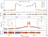 |
Fig. 1. Light curve of the lensing event KMT-2022-BLG-1479. Two lower: Overall light curve and the residuals from the model. Two upper panels: Magnified view of the anomaly region. The curve overlaid on the data points represents the best-fit 2L1S model (higher-order model with u0 > 0), which incorporates higher-order effects. The colors of the data points correspond to the labels in the legend. The two insets in the lower panel display scatter plots of points from the MCMC chain in the πE, E–πE, N parameter plane for the u0 > 0 and u0 < 0 solutions. Points within 1σ, 2σ, 3σ, 4σ, and 5σ confidence levels are marked in red, yellow, green, cyan, and blue, respectively. |
We began modeling the light curve using a static 2L1S configuration, which resulted in a unique solution with binary parameters (s, q)∼(0.78, 0.60) and an event timescale of tE ∼ 51 days. Given the relatively long duration of the event, we examined whether incorporating higher-order effects would improve the fit. This led to a model that provided a significantly better fit than the static model, with an improvement of Δχ2 = 217.0. In Table 2 we present the model parameters for both the static and higher-order models, along with their respective χ2 values. Between the two higher-order solutions, the one with u0 > 0 provides a slightly better fit to the data. The inclusion of higher-order effects results in a slight adjustment of the lensing parameters to (s, q, tE)∼(0.83, 0.60, 46 days). The model curve corresponding to the higher-order solution (with u0 > 0) is plotted in Fig. 1. As shown in the scatter plots of MCMC points on the (πE, E, πE, N) plane, presented in the insets of the lower panel of Fig. 1, the microlens parallax was robustly measured as (πE, N, πE, E) = (−0.246 ± 0.080, 0.0333 ± 0.0083) for the u0 > 0 solution and (πE, N, πE, E) = (0.219 ± 0.095, 0.0645 ± 0.0087) for the u0 < 0 solution. Additionally, the normalized source radius was accurately determined from the well-resolved caustics, yielding ρ = (7.262 ± 0.103)×10−3 for the u0 > 0 solution and ρ = (7.546 ± 0.116)×10−3 for the u0 < 0 solution.
Lensing parameters of KMT-2022-BLG-1479.
Figure 2 illustrates the lens system configurations corresponding to the u0 > 0 and u0 < 0 solutions, depicting the source trajectory relative to the lens components and caustics. The source trajectories of the two degenerate solutions are approximately symmetric with respect to the binary axis. The curvature in the source trajectory arises because of the microlens-parallax effect. The positions of the lens components and the shape of the caustics vary due to the lens-orbital effect, with the lens positions and caustics marked at two specific epochs indicated in the legend. The binary lens generates a single resonant caustic elongated in the direction nearly perpendicular to the binary lens axis. The source moved almost parallel to the binary axis, crossing the caustic. These caustic crossings produced the sharp spike features in the lensing light curve. The weaker bumps observed before and after these spikes occurred as the source approached the left-side and right-side cusps of the caustic.
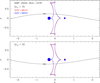 |
Fig. 2. Lens system configuration of KMT-2022-BLG-1479 for the two higher-order models with u0 > 0 and u0 < 0. In each panel, the trajectory of the source is indicated by the arrowed curve. The red and blue concave curves represent the caustics at the times specified in the legend The positions of the lens components are marked by filled dots, with the larger dot corresponding to the more massive lens component. |
3.2. KMT-2023-BLG-0932
The microlensing event KMT-2023-BLG-0932 was first identified by the KMTNet group on May 28, 2023 (HJD″ ≡ HJD − 2460000 = 92), during the initial phase of its magnification. It was later found by the MOA group on June 17 (HJD″ = 112) and by the OGLE group on July 16 (HJD″ = 141). Similar to the event KMT-2022-BLG-1479, the lensing-induced magnification persisted throughout the 2023 season and continued until the end of the 2023 observing season. In the analysis, we incorporated data from the 2024 season. The source is located in the KMTNet BLG31 field, toward which observations were made with a 2.5-hour cadence.
Figure 3 shows the lensing light curve of KMT-2023-BLG-0932. The light curve features two prominent spikes, occurring at HJD″ ∼ 187 and 198, due to caustic crossings. While the second caustic crossing was not resolved, the first crossing was captured by the combined data from the three KMTNet telescopes and the OGLE telescope. In addition to these caustic spikes, a weak bump, caused by a cusp approach, appears around HJD″ ∼ 223.
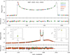 |
Fig. 3. Light curve of the lensing event KMT-2023-BLG-0932. The notations used are consistent with those presented in Fig. 1. |
From the static 2L1S modeling, we obtained a solution with binary parameters (s, q)∼(0.59, 0.96) and an event timescale of tE ∼ 77 days. However, this static model shows noticeable residuals. When higher-order effects are included, these residuals are resolved, leading to a significant improvement in the fit. The higher-order solution with u0 > 0 provides a slightly better fit than the u0 < 0 solution, with a difference of Δχ2 = 4.0. The model curve of the u0 > 0 solution is overlaid on the data points, and the full set of lensing parameters for both the static and higher-order models are listed in Table 3. The higher-order solution yields binary parameters of (s, q)∼(0.51, 1.41) and a timescale of tE ∼ 125 days. The insets of the lower panel displays scatter plots of MCMC points on the (πE, E, πE, N) plane for the two degenerate higher-order solutions. The normalized source radius was estimated from data points near the peak of the first spike, although its fractional uncertainty, dρ/ρ ∼ 4.9%, is larger than that of KMT-2022-BLG-1479 (∼1.4%), for which both caustic crossings were densely covered.
Lensing parameters of KMT-2023-BLG-0932.
Figure 4 presents the lens system configurations for the higher-order solutions with u0 > 0 and u0 < 0. In each panel, the two sets of caustics drawn in red and blue correspond to the moments of caustic entrance and exit, respectively. Since the mass ratio (q ∼ 1.4) is greater than one, the more massive lens component is located on the right side. In this event, the effect of lens orbital motion is significant, leading to a noticeable change in the caustic structure over the approximately 11-day interval between the two caustic crossings. Recently, Han et al. (2024) reported three 2L1S events exhibiting lens-orbital effects: OGLE-2018-BLG-0971, MOA-2023-BLG-065, and OGLE-2023-BLG-0136. For KMT-2023-BLG-0932, the measured rate of change in the orientation angle, α ∼ 3.1/yr, is significantly larger than those observed in the events presented in that study. The projected kinetic-to-potential energy ratio of the binary lens, calculated using Eq. (5), is (KE/PE)⊥ ∼ 0.48. The binary lens generated three caustics: a single four-cusp central caustic, shown in the figure, and a pair of small three-cusp peripheral caustics, which are not depicted and are located away from the binary lens’s barycenter. The source approached the binary-lens axis at nearly a right angle, crossing the right side of the caustic, and then moved close to the cusp of the caustic. The caustic crossings generated the observed spikes, while the cusp approach produced the subsequent bump following the caustic spikes.
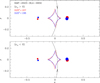 |
Fig. 4. Lens system configuration of KMT-2023-BLG-0932. Notations are consistent with those in Fig. 2. |
3.3. OGLE-2024-BLG-0142
The OGLE group initially detected the brightening of the source for the lensing event OGLE-2024-BLG-0142 on March 20, 2024 (HJD″ = 389) during its rising phase. The event was subsequently confirmed by the KMTNet group on May 3 (HJD″ = 433) and by the MOA group on May 28 (HJD″ = 458). The magnification of the source flux began before the start of the 2024 season and continued throughout it. For our analysis, we included data from both the 2023 and 2025 seasons.
The lensing light curve of the event is presented in Fig. 5. Like the previous events, it features two prominent caustic spike features at HJD″ ∼ 470 and ∼488. Both spikes were well-resolved, with the first captured by the combined data from KMTS and MOA, and the second by the combined data from KMTC and KMTS. In addition to these spikes, the light curve also shows a bump that appears before the first caustic spike, centered around HJD″ ∼ 445.
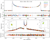 |
Fig. 5. Lensing light curve of OGLE-2024-BLG-0142 and the best-fit model. |
We initially modeled the light curve under a static 2L1S configuration, and obtained a solution with binary parameters (s, q)∼(0.73, 0.55) and an event timescale of tE ∼ 130 days. Given the long duration of the event, we further investigated a model incorporating microlens-parallax and lens-orbital effects, which resulted in a significantly improved fit with Δχ2 = 51.6. The best-fit parameters of the higher-order solution, (s, q, tE)∼(0.71, 0.57, 140), show slight variations from those of the static model. Table 4 lists the complete sets of lensing parameters for the static and two higher-order models with u0 > 0 and u0 < 0. The u0 < 0 model provides a slightly better fit than the u0 > 0 solution, with an improvement of Δχ2 = 1.7. Figure 5 presents the model light curve of the u0 < 0 higher-order solution along with its residuals, while the two insets in the lower panel displays the scatter plots of MCMC points in the (πE, E, πE, N) parameter space for the two degenerate higher-order solutions.
Lensing parameters of OGLE-2024-BLG-0142.
Figure 6 illustrates the lens system configuration for the two higher-order solutions with u0 > 0 and u0 < 0. Since the binary separation is smaller than the Einstein radius, the binary lens generates three caustics aligned perpendicular to the binary axis. The figure displays the central caustic, while the two peripheral caustics are not shown. The source passed through the central caustic, producing the two caustic-induced spikes in the light curve. Before entering the caustic, the source approached the left-side on-axis cusp, generating a bump around HJD″ ∼ 445. We present two sets of caustics corresponding to the times of the bump and the second spike, separated by approximately 38 days. The influence of lens-orbital effects on the caustic structure is minimal, resulting in only slight changes during this period.
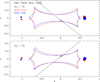 |
Fig. 8. Lens system configuration of KMT-2024-BLG-1309. |
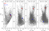 |
Fig. 9. Source locations (blue dots) on the instrumental CMDs. The centroids of the RGC are also marked, serving as reference points for color and magnitude calibration. |
3.4. KMT-2024-BLG-1309
The microlensing event KMT-2024-BLG-1309 was observed by all three active survey groups. It was first detected by the KMTNet group on June 1, 2024 (HJD″ = 472), with subsequent detection by the OGLE group on June 17 (HJD″ = 478) and the MOA group on July 11 (HJD″ = 502). The source star has an I-band baseline magnitude of Ibase = 19.16 and is located in a field monitored with a high observational cadence. As a result, the event’s light curve was densely sampled, providing detailed coverage of its magnification features.
Figure 7 shows the lensing light curve of KMT-2024-BLG-1309, which features two prominent caustic spikes at HJD″ ∼ 503.0 and 516.8, along with two bumps at HJD″ ∼ 482 before the first spike and at HJD″ ∼ 538 after the second caustic feature. Both caustic spikes were clearly resolved, with the first spike captured by the MOA and KMTS datasets, and the second spike observed by the OGLE, KMTC, and MOA datasets. Although the entire lensing magnification event occurred within the 2024 season, it lasted for a significant period of time.
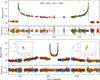 |
Fig. 7. Lensing light curve of KMT-2024-BLG-1309 and the best-fit model. |
We modeled the light curve under both a static 2L1S configuration and a configuration that accounts for higher-order effects. The lensing parameters derived from the two models are similar, with values of (s, q, tE)∼(1.63, 1.64, 45 days). Incorporating higher-order effects leads to an improved fit, reducing the chi-square value by Δχ2 = 38.2. The scatter plot of the MCMC points on the (πE, E, πE, N) plane for both solutions with u0 > 0 and u0 < 0 are presented in the inset of the lower panel of Fig. 7. A full sets of lensing parameters for both the static and higher-order models are provided in Table 5. The model light curve obtained from the higher-order modeling (with u0 > 0) is overlaid on the observational data.
Lensing parameters of KMT-2024-BLG-1309.
Figure 8 shows the lens-system configurations corresponding to the u0 > 0 (upper panel) and u0 < 0 (lower panel) solutions. The lens creates a single resonant caustic that extends along the binary-lens axis. The observed caustic spikes occurred as the source traversed diagonally across the central region of the caustic. Before entering the caustic in the u0 < 0 case, the source approached an upper cusp, and after exiting, it moved toward a lower cusp on the opposite side. These cusp interactions lead to the formation of bumps in the light curve at the corresponding times.
4. Source stars and angular Einstein radii
In this section we specify the source stars to fully characterize the events and estimate the angular Einstein radii. The source of each event is defined by measuring its V − I color and I-band magnitude. After calibrating these values using the procedure outlined below, we estimated the angular source radius (θ*) based on the calibrated color and magnitude. With the estimated θ*, we calculated the angular Einstein radius using the relationship in Eq. (2), along with the normalized source radius ρ derived from light curve modeling. The following provides a detailed, step-by-step description of the procedure for measuring θE.
In the first step, we measured the instrumental source magnitudes in the V and I passbands. To do this, we created two light curves from the data measured in these passbands, which were processed using the pyDIA code developed by Albrow (2017). From these light curves, we determined the instrumental flux of the source (Fs) in each band by fitting the observed flux (Fobs) to the model (Amodel):
 (6)
(6)
Here, Fb represents the blended flux. Figure 9 illustrates the source locations in the instrumental color-magnitude diagrams (CMDs), which were constructed using pyDIA photometry of stars located near the source.
The source color and magnitude were calibrated based on their position in the CMD. For this calibration, the centroid of the red giant clump (RGC) in the CMD was used as a reference (Yoo et al. 2004), as its de-reddened color and magnitude, (V − I, I)RGC, 0, corrected for extinction, had been previously determined by Bensby et al. (2013) and Nataf et al. (2013). By measuring the color and magnitude offset, Δ(V − I, I), between the source and the RGC centroid, the de-reddened source color and magnitude were calculated as
 (7)
(7)
Table 6 lists the instrumental color and magnitude of the source, (V − I, I)s, and the RGC centroid, (V − I, I)RGC, along with the de-reddened values for both the RGC, (V − I)RGC, 0, and the source, (V − I, I)s, 0, for each event. Based on the estimated colors and magnitudes, the source stars are classified as follows: a K-type giant for KMT-2022-BLG-1479, a K-type subgiant for KMT-2023-BLG-0932, an early K-type main-sequence star for OGLE-2024-BLG-0142, and an early G-type main-sequence star for KMT-2024-BLG-1309.
Source parameters, angular Einstein radii, and relative lens-source proper motions.
The angular radius of the source star was determined using the estimated color and magnitude. This was achieved by applying the relation between θ* and (V − K, K) provided by Kervella et al. (2004). To utilize this relation, the V − I color was converted to V − K using the color-color relation from Bessell & Brett (1988), enabling the derivation of θ*. With the angular source radius estimated, the angular Einstein radius, θE, was calculated using the relation in Eq. (2). Combined with the event timescale obtained from the modeling, the relative lens-source proper motion, μ, was determined as
 (8)
(8)
The derived values of θ*, θE, and μ for the events are provided in the last three rows of Table 6.
Physical lens parameters.
5. Physical lens parameters
Using the lensing observables tE, θE, and πE, we derived the physical parameters of the lens mass and distance based on the relationships described in Eq. (4). The determined physical lens parameters, including the masses of the binary lens components (M1 and M2), the lens distance (DL), and the projected separation between the lens components (a⊥), corresponding to the u0 > 0 and u0 < 0 solutions are presented in Table 7. The projected separation is calculated using the equation
 (9)
(9)
where the normalized source radius s is obtained from the modeling process. For the estimation of the physical parameters, we assumed the distance to the source to be DS = 8 kpc. Note, however, that the mass estimates, M = θE/(κπE), are independent of the assumed source distances. Although some variations exist, the physical parameters estimated from the u0 > 0 and u0 < 0 solutions remain consistent.
The masses of the lens components vary across different events. In the cases of KMT-2022-BLG-1479, KMT-2023-BLG-0932, and KMT-2024-BLG-1309, both components of the binary lens are less massive than the Sun, with their masses aligning with those of M-type dwarfs, which are the most common type of lenses in Galactic microlensing events (Han & Gould 2003). In contrast, for OGLE-2024-BLG-0142, the primary lens component has a mass comparable to that of the Sun, while the companion lens component has a mass approximately half that of the primary.
The distances to the lenses also vary across different events. For KMT-2022-BLG-1479, KMT-2023-BLG-0932, and KMT-2024-BLG-1309, the lenses are located at relatively close distances, with DL ≲ 2.7 kpc, suggesting that these lenses are situated within the Galactic disk. In contrast, the lens for OGLE-2024-BLG-0142 is located farther away, with a distance of DL ∼ 4.8 kpc for the u0 > 0 solution and DL ∼ 4.4 kpc for the u0 < 0 solution, which is significantly greater than that of the other events. Bayesian analysis, incorporating Galactic model priors, indicates that the lens for OGLE-2024-BLG-0142 has a 35% probability of being in the disk and a 65% probability of being in the bulge.
6. Summary and conclusion
We analyzed binary lens events detected from microlensing surveys from 2022 to 2024 seasons to identify those suitable for lens mass measurements. Our investigation focused on two key features in lensing light curves. The first feature is distinct caustic spikes with resolved crossings, which enable the measurement of the angular Einstein radius (θE). The second feature is long event durations, which enable the determination of the microlens parallax (πE). Based on these criteria, we identified four qualifying events, KMT-2022-BLG-1479, KMT-2023-BLG-0932, OGLE-2024-BLG-0142, and KMT-2024-BLG-1309.
Detailed modeling of the events revealed that the lenses are binary systems with mass ratios between 0.5 and 0.7. For all events, in addition to the basic event timescale, the extra observables of the angular Einstein radius and microlens parallax were securely measured. The angular Einstein radius was derived by combining the normalized source radius obtained from modeling the resolved caustic spikes with the angular source radius estimated from the source color and magnitude. The microlens parallax was determined through light curve modeling, accounting for higher-order effects induced by the orbital motions of Earth and the binary lens.
By combining the event timescale, angular Einstein radius, and microlens parallax, the mass and distance of the lens were uniquely determined. In the cases of KMT-2022-BLG-1479, KMT-2023-BLG-0932, and KMT-2024-BLG-1309, both components of the binary lens have masses below that of the Sun, consistent with M-type dwarfs, which are the most frequently observed lenses in Galactic microlensing events. These lenses are located relatively close, at distances of less than 2.7 kpc, suggesting their presence within the Galactic disk. For OGLE-2024-BLG-0142, the primary lens component has a mass similar to that of the Sun, while the companion lens component has about half the mass of the primary. This lens system is located at a greater distance, approximately 4.4 kpc for one solution and 4.8 kpc for the other.
For a comparison between the physical parameters of the current events and those of previously reported events with measured annual parallaxes (as discussed in Sect. 1), we present their respective lens masses and distances in Table 8. From this comparison, two notable trends emerge. First, the lens masses are generally not high, despite the long timescales of the events. This indicates that the extended durations are primarily due to a combination of slow lens-source proper motions and large angular Einstein radii, rather than being driven by massive lenses, as previously argued by Han et al. (2018). Second, most lenses are located at relatively close distances, typically within DL ≲ 5 kpc. This suggests that they predominantly reside in the Galactic disk, although for the overall microlensing event population, the contribution from bulge lenses generally exceeds that of disk lenses (Han & Gould 2003). This tendency is expected because nearby lenses generally exhibit larger microlens parallaxes, which facilitates their characterization.
Previous events with physical lens parameters.
The results of our binary-lens events analyses suggest that the upcoming gravitational microlensing experiment using the Nancy Grace Roman Space Telescope (Spergel et al. 2015) will enable the determination of lens masses in many binary-lens events. While the primary focus of the Roman microlensing survey is the detection of distant exoplanets, including those with masses lower than Earth’s, it will also uncover numerous binary-lens events with densely resolved, high-precision light curves, made possible by the telescope’s excellent photometric accuracy and 15-minute cadence of space-based observations. For many of these events, as shown in this study, the physical properties of the lens are expected to be directly measurable.
Acknowledgments
This research was supported by the Korea Astronomy and Space Science Institute under the R&D program (Project No. 2025-1-830-05) supervised by the Ministry of Science and ICT. This research has made use of the KMTNet system operated by the Korea Astronomy and Space Science Institute (KASI) at three host sites of CTIO in Chile, SAAO in South Africa, and SSO in Australia. Data transfer from the host site to KASI was supported by the Korea Research Environment Open NETwork (KREONET). C.Han acknowledge the support from the Korea Astronomy and Space Science Institute under the R&D program (Project No. 2025-1-830-05) supervised by the Ministry of Science and ICT. J.C.Y., I.G.S., and S.J.C. acknowledge support from NSF Grant No. AST-2108414. W.Zang acknowledges the support from the Harvard-Smithsonian Center for Astrophysics through the CfA Fellowship. The MOA project is supported by JSPS KAKENHI Grant Number JP16H06287, JP22H00153 and 23KK0060. C.R. was supported by the Research fellowship of the Alexander von Humboldt Foundation.
References
- Albrow, M. 2017, https://doi.org/10.5281/zenodo.268049 [Google Scholar]
- Albrow, M. D., Beaulieu, J.-P., Caldwell, J. A. R., et al. 1999, ApJ, 522, 1022 [NASA ADS] [CrossRef] [Google Scholar]
- Albrow, M. D., Beaulieu, J.-P., Caldwell, J. A. R., et al. 2000, ApJ, 534, 894 [NASA ADS] [CrossRef] [Google Scholar]
- Albrow, M., Horne, K., Bramich, D. M., et al. 2009, MNRAS, 397, 2099 [Google Scholar]
- An, J. H., & Gould, A. 2001, ApJ, 563, L111 [Google Scholar]
- An, J. H., & Han, C. 2002, ApJ, 573, 351 [NASA ADS] [CrossRef] [Google Scholar]
- An, J. H., Albrow, M. D., Beaulieu, J.-P., et al. 2002, ApJ, 572, 521 [NASA ADS] [CrossRef] [Google Scholar]
- Batista, V., Dong, S., Gould, A., et al. 2009, A&A, 508, 467 [NASA ADS] [CrossRef] [EDP Sciences] [Google Scholar]
- Batista, V., Gould, A., Dieters, S., et al. 2011, A&A, 529, A102 [NASA ADS] [CrossRef] [EDP Sciences] [Google Scholar]
- Bensby, T., Yee, J. C., Feltzing, S., et al. 2013, A&A, 549, A147 [NASA ADS] [CrossRef] [EDP Sciences] [Google Scholar]
- Bessell, M. S., & Brett, J. M. 1988, PASP, 100, 1134 [Google Scholar]
- Bond, I. A., Abe, F., Dodd, R. J., et al. 2001, MNRAS, 327, 868 [Google Scholar]
- Calchi Novati, S., Suzuki, D., Udalski, A., et al. 2019, AJ, 157, 121 [Google Scholar]
- Choi, J.-Y., Shin, I.-G., Park, S.-Y., et al. 2012, ApJ, 751, 41 [Google Scholar]
- Claret, A. 2000, A&A, 363, 1081 [NASA ADS] [Google Scholar]
- Dong, S., DePoy, D. L., Gaudi, B. S., et al. 2006, ApJ, 642, 842 [NASA ADS] [CrossRef] [Google Scholar]
- Doran, M., & Mueller, C. M. 2004, J. Cosmol. Astropart. Phys., 09, 003 [CrossRef] [Google Scholar]
- Gould, A. 1992, ApJ, 392, 442 [Google Scholar]
- Gould, A. 1994, ApJ, 421, L71 [NASA ADS] [CrossRef] [Google Scholar]
- Gould, A. 2000, ApJ, 542, 785 [NASA ADS] [CrossRef] [Google Scholar]
- Gould, A. 2004, ApJ, 606, L319 [CrossRef] [Google Scholar]
- Gould, A., & Horne, K. 2013, ApJ, 779, L28 [Google Scholar]
- Han, C., & Gould, A. 2003, ApJ, 592, 172 [Google Scholar]
- Han, C., Jung, Y. K., Shvartzvald, Y., et al. 2018, ApJ, 865, 14 [Google Scholar]
- Han, C., Udalski, A., & Bond, I. A. 2024, A&A, 686, A234 [NASA ADS] [CrossRef] [EDP Sciences] [Google Scholar]
- Herald, A., Udalski, A., Bozza, V., et al. 2022, A&A, 663, A100 [NASA ADS] [CrossRef] [EDP Sciences] [Google Scholar]
- Hwang, K.-H., Han, C., Bond, I. A., et al. 2010, ApJ, 717, 435 [Google Scholar]
- Jaroszyński, M., Udalski, A., Kubiak, M., et al. 2005, Acta Astron., 55, 159 [Google Scholar]
- Jiang, G., DePoy, D. L., Gal-Yam, A., et al. 2004, ApJ, 617, 1307 [Google Scholar]
- Jung, Y. K., Han, C., Bond, I. A., et al. 2019, ApJ, 872, 175 [Google Scholar]
- Kervella, P., Thévenin, F., Di Folco, E., & Ségransan, D. 2004, A&A, 426, 29 [Google Scholar]
- Kim, S.-L., Lee, C.-U., Park, B.-G., et al. 2016, JKAS, 49, 37 [Google Scholar]
- Malpas, A., Albrow, M. D., Yee, J. C., et al. 2022, AJ, 164, 102 [NASA ADS] [CrossRef] [Google Scholar]
- Mao, S., & Paczyński, B. 1991, ApJ, 374, 37 [Google Scholar]
- Nataf, D. M., Gould, A., Fouqué, P., et al. 2013, ApJ, 769, 88 [Google Scholar]
- Nemiroff, R. J., & Wickramasinghe, W. A. D. T. 1994, ApJ, 424, L21 [NASA ADS] [CrossRef] [Google Scholar]
- Pejcha, O., & Heyrovský, D. 2009, ApJ, 690, 1772 [NASA ADS] [CrossRef] [Google Scholar]
- Poindexter, S., Afonso, C., Bennett, D. P., et al. 2005, ApJ, 633, 914 [NASA ADS] [CrossRef] [Google Scholar]
- Schneider, P., & Weiss, A. 1986, A&A, 164, 237 [NASA ADS] [Google Scholar]
- Shin, I.-G., Han, C., Choi, J.-Y., et al. 2012, ApJ, 755, 91 [Google Scholar]
- Shin, I.-G., Udalski, A., Yee, J. C., et al. 2017, AJ, 154, 76 [NASA ADS] [CrossRef] [Google Scholar]
- Skowron, J., Udalski, A., Gould, A., et al. 2011, ApJ, 738, 87 [Google Scholar]
- Spergel, D., Gehrels, N., Baltay, C., et al. 2015, arXiv e-prints [arXiv:1503.03757] [Google Scholar]
- Sumi, T., Abe, F., Bond, I. A., et al. 2003, ApJ, 591, 204 [NASA ADS] [CrossRef] [Google Scholar]
- Udalski, A. 2003, Acta Astron., 53, 291 [NASA ADS] [Google Scholar]
- Udalski, A., Szymański, M. K., & Szymański, G. 2015, Acta Astron., 65, 1 [NASA ADS] [Google Scholar]
- Wang, T., Zhu, W., Mao, S., et al. 2017, ApJ, 845, 129 [Google Scholar]
- Witt, H. J., & Mao, S. 1994, ApJ, 430, 505 [NASA ADS] [CrossRef] [Google Scholar]
- Yang, H., Yee, J. C., Hwang, K.-H., et al. 2024, MNRAS, 528, 11 [NASA ADS] [CrossRef] [Google Scholar]
- Yee, J. C., Shvartzvald, Y., Gal-Yam, A., et al. 2012, ApJ, 755, 102 [Google Scholar]
- Yoo, J., DePoy, D. L., Gal-Yam, A., et al. 2004, ApJ, 603, 13 [Google Scholar]
- Zhu, W., Udalski, A., Gould, A., et al. 2015, ApJ, 805, 8 [Google Scholar]
All Tables
Source parameters, angular Einstein radii, and relative lens-source proper motions.
All Figures
|
Fig. 1. Light curve of the lensing event KMT-2022-BLG-1479. Two lower: Overall light curve and the residuals from the model. Two upper panels: Magnified view of the anomaly region. The curve overlaid on the data points represents the best-fit 2L1S model (higher-order model with u0 > 0), which incorporates higher-order effects. The colors of the data points correspond to the labels in the legend. The two insets in the lower panel display scatter plots of points from the MCMC chain in the πE, E–πE, N parameter plane for the u0 > 0 and u0 < 0 solutions. Points within 1σ, 2σ, 3σ, 4σ, and 5σ confidence levels are marked in red, yellow, green, cyan, and blue, respectively. |
| In the text | |
|
Fig. 2. Lens system configuration of KMT-2022-BLG-1479 for the two higher-order models with u0 > 0 and u0 < 0. In each panel, the trajectory of the source is indicated by the arrowed curve. The red and blue concave curves represent the caustics at the times specified in the legend The positions of the lens components are marked by filled dots, with the larger dot corresponding to the more massive lens component. |
| In the text | |
|
Fig. 3. Light curve of the lensing event KMT-2023-BLG-0932. The notations used are consistent with those presented in Fig. 1. |
| In the text | |
|
Fig. 4. Lens system configuration of KMT-2023-BLG-0932. Notations are consistent with those in Fig. 2. |
| In the text | |
|
Fig. 5. Lensing light curve of OGLE-2024-BLG-0142 and the best-fit model. |
| In the text | |
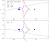 |
Fig. 6. Lens-system configuration of OGLE-2024-BLG-0142. Notations are same as those in Fig. 2. |
| In the text | |
|
Fig. 8. Lens system configuration of KMT-2024-BLG-1309. |
| In the text | |
|
Fig. 9. Source locations (blue dots) on the instrumental CMDs. The centroids of the RGC are also marked, serving as reference points for color and magnitude calibration. |
| In the text | |
|
Fig. 7. Lensing light curve of KMT-2024-BLG-1309 and the best-fit model. |
| In the text | |
Current usage metrics show cumulative count of Article Views (full-text article views including HTML views, PDF and ePub downloads, according to the available data) and Abstracts Views on Vision4Press platform.
Data correspond to usage on the plateform after 2015. The current usage metrics is available 48-96 hours after online publication and is updated daily on week days.
Initial download of the metrics may take a while.